Investigating Snow Cover and Hydrometeorological Trends in Contrasting Hydrological Regimes of the Upper Indus Basin

Institute of Geographical Information Systems, National University of Sciences and Technology (NUST), Islamabad 44000, Pakistan
*
Author to whom correspondence should be addressed.
Atmosphere 2018, 9(5), 162; https://doi.org/10.3390/atmos9050162
Submission received: 7 March 2018
/
Revised: 22 April 2018
/
Accepted: 23 April 2018
/
Published: 26 April 2018
(This article belongs to the Section Meteorology)
Abstract
:The Upper Indus basin (UIB) is characterized by contrasting hydrometeorological behaviors; therefore, it has become pertinent to understand hydrometeorological trends at the sub-watershed level. Many studies have investigated the snow cover and hydrometeorological modeling at basin level but none have reported the spatial variability of trends and their magnitude at a sub-basin level. This study was conducted to analyze the trends in the contrasting hydrological regimes of the snow and glacier-fed river catchments of the Hunza and Astore sub-basins of the UIB. Mann-Kendall and Sen’s slope methods were used to study the main trends and their magnitude using MODIS snow cover information (2001–2015) and hydrometeorological data. The results showed that in the Hunza basin, the river discharge and temperature were significantly (p ≤ 0.05) decreased with a Sen’s slope value of −2.541 m3·s−1·year−1 and −0.034 °C·year−1, respectively, while precipitation data showed a non-significant (p ≥ 0.05) increasing trend with a Sen’s slope value of 0.023 mm·year−1. In the Astore basin, the river discharge and precipitation are increasing significantly (p ≤ 0.05) with a Sen’s slope value of 1.039 m3·s−1·year−1 and 0.192 mm·year−1, respectively. The snow cover analysis results suggest that the Western Himalayas (the Astore basin) had a stable trend with a Sen’s slope of 0.07% year−1 and the Central Karakoram region (the Hunza River basin) shows a slightly increasing trend with a Sen’s slope of 0.394% year−1. Based on the results of this study it can be concluded that since both sub-basins are influenced by different climatological systems (monsoon and westerly), the results of those studies that treat the Upper Indus basin as one unit in hydrometeorological modeling should be used with caution. Furthermore, it is suggested that similar studies at the sub-basin level of the UIB will help in a better understanding of the Karakoram anomaly.
1. Introduction
Pakistan’s economy is dependent on agriculture, which is reliant on water flow from the Indus River and its tributaries. The water supply to the agricultural lands of Punjab and Sindh is from the main Terbela reservoir of the Indus River, which receives its main contribution from the snow and glacier melt from the Upper Indus basin (UIB) [1].
The UIB has a total area of greater than 200,000 km2 [2,3] and is divided into five sub-basins as Shyok, Shigar, Astore, Gilgit and Hunza that receive about 60% of the meltwater from glaciers and snow [4]. These sub-basins are highly influenced by the westerly weather system with limited effects from monsoons. As the population living downstream and other economic activities are highly dependent on these water resources, so it is vital to assess how the water resources in these basins will behave under future climate change scenarios. Several studies have been conducted to evaluate the climate change impact on the water resources of the UIB. For example, Archer [5] studied the high-elevation tributaries of the UIB and found a strong association between summer runoff and summer mean temperature. He, along with Forsythe et al. [6] indicated that a single degree rise in mean summer temperature might result in an approximately 10–20% increase in summer runoff in the Hunza basin. Tahir et al. [2] found that a 1 °C rise in mean annual temperature may force the mean annual discharge in the Hunza basin to increase by about 32% in next few years. If these scenarios hold true, then the glaciers may retreat, generate a high volume of water over a few decades but later lead to a longer period of water scarcity. Hewitt [3,4] reported that there is a five- to ten-fold increase in precipitation over an elevation of 5000 m with a significant drop in temperature. Winiger et al. [7] assessed the total annual precipitation for different altitudinal zones of the UIB using a combined snow cover and ablation model. They found that the Karakoram Range received maximum precipitation at an elevation of above 5500 m, whereas high elevation (4000 m) regions generate much of the UIB’s flow [5,8]. However, only a few studies, e.g., [9,10] have monitored the climatic parameters, snow and ice processes and resultant hydrological regimes at these altitudes.
There is a growing consensus that long-term changes in temperature and rainfall may alter the hydrometeorological and ecological processes of a region [11]. Over the past few years, many studies have been conducted worldwide to assess the changing trends in temperature and rainfall for different countries such as the USA, Africa, India, Norwegian Arctic, Nepal, Northwestern Himalaya [10,12,13,14,15], using different statistical models and methods.
Trend investigation in climatic data is a conventional process to analyze the climate variability of any region, as it portrays all variations over time [16]. Trend analysis does not explain the factors and internal dynamics of climate variability but it shows the overall change in magnitude and direction. Attributes like auto-correlation and seasonality in data are problematic for the quantification of long-term trends [12]. These problems can be resolved by using a trend-free pre-whitening approach (TFPW) [17], which helps to eliminate the seasonality in data before implementation of any test for trend detection. Another approach is to practice those tests that are not affected by the seasonal cycles [18]. In general, two types of statistical approaches are practiced as found in the literature [19,20], i.e., parametric (linear regression) and non-parametric (Mann-Kendall and Sen’s slope estimator) [21,22]. Parametric tests have been used widely by many researchers due to their simplicity. These are appropriate when a scatter plot of the time series data gives linear (increasing or decreasing) trends with few outliers. The t-test can be applied to quantify the significance of the slope of the regression line but these tests are not applicable when skewness or auto-correlation exists in the data (i.e., seasonal cycles). Moreover, t-tests may produce a misleading statistically significant slope when the actual slope is zero [23]. When compared with the t-test, the non-parametric Mann-Kendall (M-K) test is more applicable in the case of skewed distribution of the data. However, the M-K test is computationally extensive as it requires the elimination of seasonal cycles. Sen’s slope non-parametric estimator [21] is the best method to analyze the magnitude of a trend in time series data. This method assumes that the trend line is a linear function in the time series data. In Sen’s slope model, the slope value shows the increase and decrease of the variable [24]. Another benefit of using Sen’s slope is that it is not affected when outliers and single data errors are present in the dataset [25]. Using these statistical approaches, there is a pressing need to assess the impact of climate change on the water resources of the UIB. The UIB is well known for the non-availability or limited availability of long-term (over 30 years) hydrometeorological ground data and high-altitude data scarcity, although there are studies which have used limited time series data (10–15 years) to determine trends [26,27,28,29,30]. Saavedra et al. [30] applied the nonparametric Mann-Kendall statistics to 16 years of snow cover data (2000–2016) to assess the trends of snow persistence in the Andes. Another study conducted by Kumar et al. [28] analyzed the trends in maximum, minimum, and mean temperatures in the western Indian Himalaya by applying nonparametric statistics, i.e., the Mann-Kendall test was applied to monthly data from 2000 to 2014. Hydrometeorological parameters such as maximum, minimum, and mean temperature, precipitation, snowfall and river discharge should be studied to assess the current and future trends in variability. Hydrometeorological stations can provide the ground data for any region with limited spatial coverage, as it is difficult to install an observatory in an entire area. Even with this limitation, hydrometeorological stations can provide data for temperature, precipitation and discharge at low altitudes of the UIB, although it is difficult to record data because most of the snowfall is at higher altitude. In remote regions, such as the UIB, satellite remote-sensing techniques may be the only way to analyze spatiotemporal variations in snow cover [2,31]. Moderate Resolution Imaging Spectroradiometer (MODIS) snow products have been widely used in estimating the spatial extent of snow cover and in snowmelt runoff modeling applications [2,9]. Several studies have compared the relatively “coarse” resolution (500 m) MODIS data with the “fine” resolution (30 m) Advanced Spaceborne Thermal Emission and Reflection Radiometer (ASTER) data and ground observations in estimating snow cover; the MODIS presented satisfactory results at both low and high altitudes [2]. The overall absolute accuracy of the 500 m resolution of MODIS snow products is 90% [31], but this varies by land-cover type and snow condition. These findings also support the use of MODIS data in estimating changes in snow cover extent at varying altitudes of the UIB.
Many studies [19,32] have reported trend analysis of hydrometeorological variables along with MODIS snow product at the basin level, which provides a general trend at the large scale. However, these studies did not address the variability of hydrometeorological variables at the sub-basin scale. Also, none of these studies reported the spatial variability and magnitude of the trend. Thus, this study was designed to investigate the spatiotemporal variability and trends of several hydrometeorological variables including temperature, precipitation and river discharge in the Hunza and Astore sub-basins of the UIB. This study provides a comprehensive overview of hydrometeorological statistics, including the seasonal and internal variability of contrasting regimes at the sub-basin level of the UIB using nonparametric Mann-Kendall and Sen’s slope statistical methods.
2. Materials and Methods
2.1. Study Area
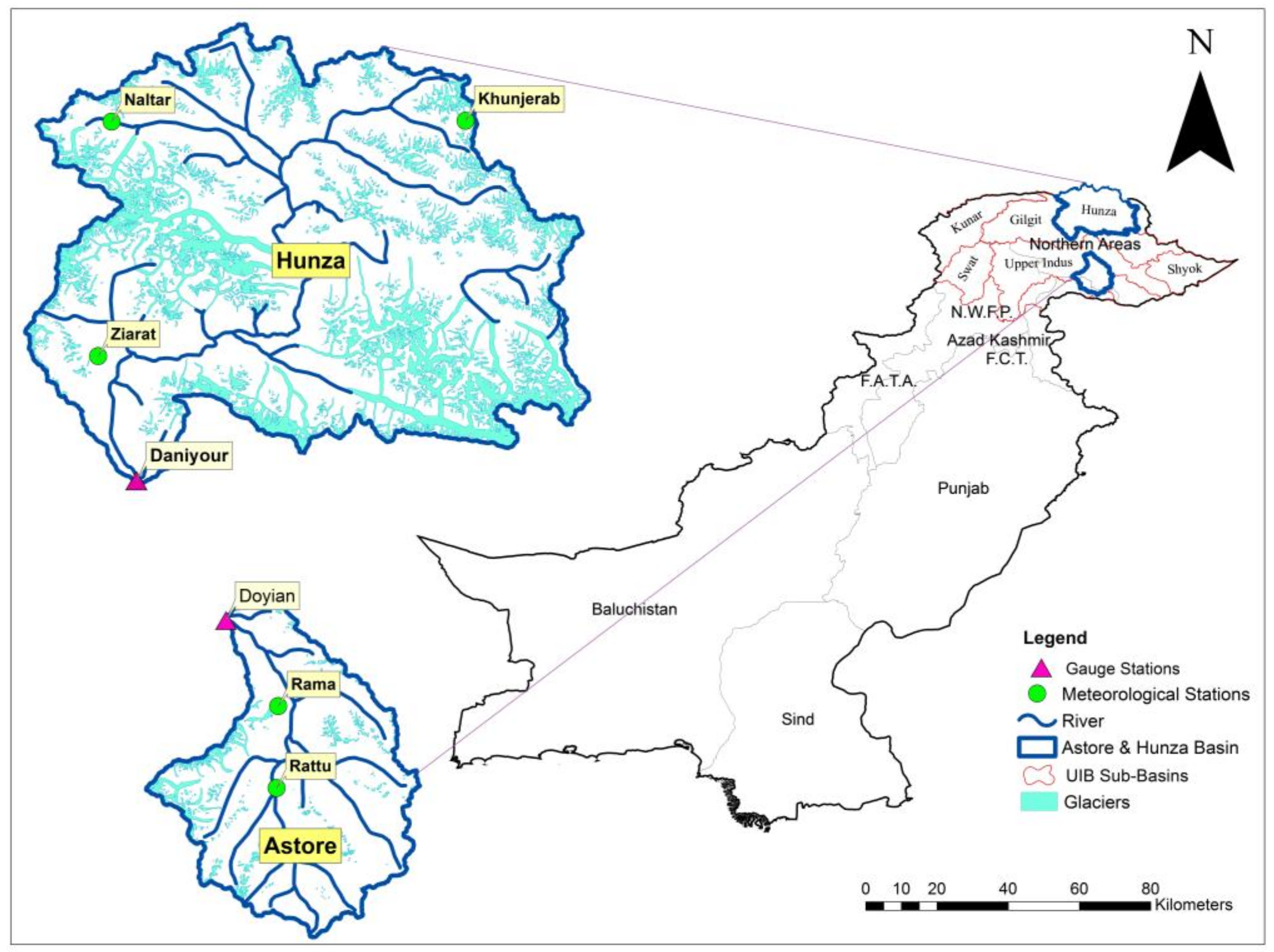
The Astore and Hunza sub-basins of the UIB were selected based on their contrasting hydrometeorological regimes (Figure 1). Both catchments come under the influence of Westerlies, but in slightly different ways, regardless of their spatial relationship. The Hunza River flow is profoundly influenced by Westerlies which bring maximum precipitation in winter in the form of snow and generate maximum flow in summer due to snow melting. The Astore River flow is influenced by monsoonal rainfall with little contribution by the Westerlies [1,2,10]. The Astore basin mean altitude is approx. 4100 m, which is lower compared to that of the Hunza basin’s mean altitude of about 4650 m. About 33% of the area of the Hunza basin lies above 5000 m, whereas this percentage is about 5% in the Astore basin.
2.2. Data Utilized
The study considers meteorological data gathered at five stations over 14 years (1999–2012) and hydrological data (1966–2012) for the Hunza River at Dainyor, and the Astore River at Doyian. Data availability at the lower stations and data scarcity at high altitude in the UIB were major constraints in this study. This issue has been highlighted by many [33]. The few stations that are present at high altitude has been reported to underestimate the solid precipitation due to high winds [2]. However, snow cover was analyzed over 15 years (2001–2015), using the MODIS 8-day snow product. Spatio-temporal maps of hydrometeorological trends and their magnitude were generated using nonparametric Mann-Kendall and Sen’s slope statistical methods.
2.2.1. Hydrometeorological Data
Long-term daily data of maximum and minimum temperature, precipitation and discharge were collected from two flow gauge stations (Daniyor Bridge in Hunza and Doyian in Astore) and five meteorological stations (Khunjerab, Ziarat, Naltar in Hunza and Rama, Rattu in Astore) in the study area (Figure 1).
The monthly mean of the daily maximum, minimum and average temperatures, precipitation and discharge was calculated for each of the years (1999–2012). Daily average temperature is based on the arithmetic mean of the daily maximum and minimum temperatures. Unrecorded data was replaced by interpolating the successive and preceding year’s data. The mean temperature of Hunza and Astore was 1.4 °C and 6 °C, respectively, whereas, Hunza received less precipitation than Astore, with a daily mean value of 1 mm and 2.15 mm, respectively.
2.2.2. Snow Cover Data
In general, in situ snow monitoring stations are very limited in the Himalaya region and particularly in the Upper Indus basin. Even where they are present, the station data represents only point information; besides which, only one or two stations are present at high altitude. The Karakoram receives maximum precipitation at elevations above 5000 m [7,34]. Due to this point-based information, the snow data is not representative of the larger area and thus it is not suitable for basin-level snow analysis. However, remote sensing data has an edge due to its continuous (spatially and temporally) coverage of snow-covered regions and therefore it can be used to assess the spatiotemporal variability and trends of snow at basin level. Wake [8] argued that solid precipitation adds a large moisture surplus to the UIB in the form of snow. Since the meteorological stations at high altitude can only capture 20–30% of the precipitation, with the remaining dispersed by gusty winds [2], this might be a reason for the low precipitation recorded at the Khunjerab meteorological station located just below 5000 m. Lal [35] and Førland et al. [36] argued that squalls, wetting loss, trace precipitation, and blowing and drifting of snow are the main contributing factors for precipitation not being recorded correctly at meteorological gauge stations. Due to these uncertainties in recorded precipitation, remote sensing-based snow cover estimation is the most appropriate choice for reliable results.
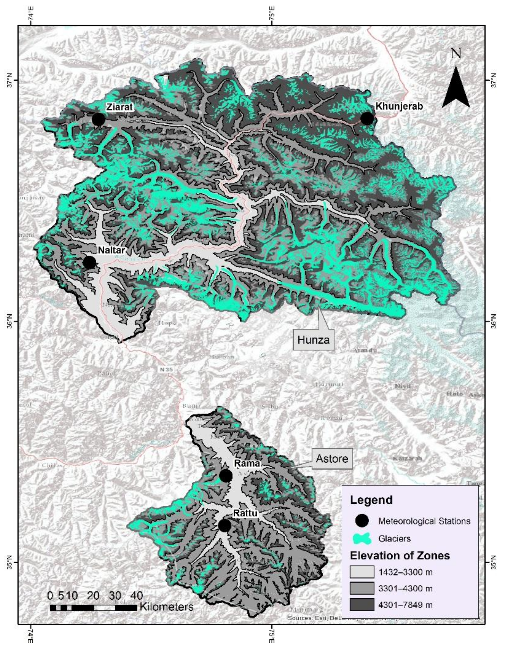
Hence, the Moderate Resolution Imaging Spectroradiometer (MODIS/Terra Snow Cover 8-Day L3 Global 500 m Grid (MOD10A2) snow product was used to quantify the spatiotemporal trend in the snow cover of the Astore and Hunza basins. The MODIS 8-day product is an integration of the daily MODIS product and several researchers have suggested that it seems to produce better results than the daily product [37,38,39,40]. It had a spatial resolution of 500 m which was interpolated using the IDW technique in ArcGIS software (ver. 10.4). A total of 630 images of MODIS, MOD10A2 snow product were downloaded (https://modis.gsfc.nasa.gov/data/dataprod/mod10.php) for the 15-year period from 2001–2015 for the Astore and Hunza sub-basins. The cloud cover was removed by using a validated non-spectral cloud removal technique [41] in Erdas Imagine software (ver. 2014). Geospatial analysis was performed in ArcGIS software (ver. 10.4) where the model builder module of ArcGIS was used for building a model for geoprocessing tasks, i.e., extraction of snow cover area and its quantification. The snow cover (%) at three elevation zones [42] in each sub-basin was analyzed to study the spatiotemporal trend of snow cover in each zone (Figure 2). The threshold values for the altitudinal zonal boundaries of the Astore basin were kept similar to the Hunza basin so that the basin characteristics at the same elevations could be compared (Table 1). A hypsometric curve (Appendix A) shows the cumulative distribution function of elevations of the Astore and Hunza sub-basins.
2.3. Methodology
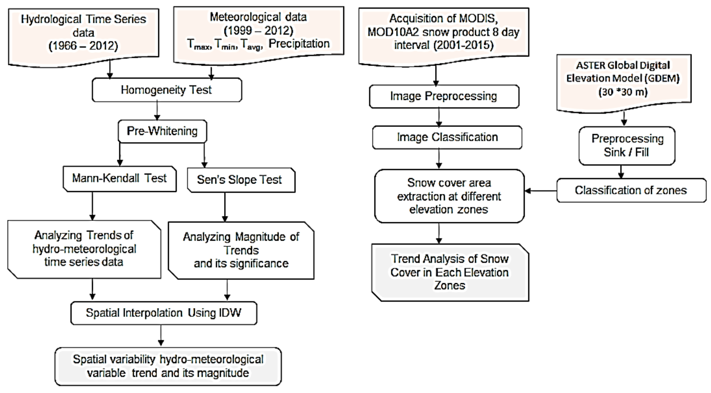
The complete methodological framework of the study is given in Figure 3. The homogeneity test was applied to the hydrological and meteorological datasets. The fill and sink operation was also applied to the digital elevation model to fill the depressions.
2.3.1. Data Homogeneity Test
The standard normal homogeneity test (SNHT) [43] was used to evaluate the homogeneity of hydrometeorological and snow cover data at a 5% significance level for each station. Data is considered to be homogeneous when the computed p-value is less than 0.05. All the hydrometeorological variables were found to be homogenous.
2.3.2. Trend Analysis
To analyze the trend in time series data it is crucial to detect the presence of serial correlation/auto-correlation in the data. Auto-correlation is the correlation of a variable with itself over successive lags (time intervals) [44]. The trend test would significantly portray inflated results, if applied without removing the auto-correlation effect. The hydrometeorological time series data was pre-whitened (removal of auto-correlation or serial correlation effect) as suggested by Yue et al. [45] before investigating the trend detection in hydrometeorological time series data.
The rank-based non-parametric Mann-Kendall test was applied to determine the trends in time series of hydrometeorological data from the Hunza and Astore sub-basins using the Minitab software (ver. 18) [46]. The null hypothesis (H0) was set to be no trend in time series data, while an alternate hypothesis (H1) was set to be an increasing or decreasing trend over time. The mathematical equations (Equations (1)–(4)) for calculating Mann-Kendall Statistics (S) and test statistics (Z) are as follows:
In the above Equations (1)–(4) Xi and Xj are the time series observations arranged in the order of occurrence, n is the length of time series, tp is the number of ties for pth value, and q is the number of tied values. The presence of a statistically significant trend is evaluated using the Z value. Positive Z value indicate an increasing trend in the time series data; negative Z values indicate a decreasing trend. If |Z| > Z1−α/2, (H0) is rejected then it is considered as the presence of a statistically significant trend in the time series data. The critical value of Z1−α/2 for a p value of 0.05 was set to be 1.96.
2.3.3. Sen’s Slope Estimator
The nonparametric Sen’s slope method was used to quantify the magnitude of the trend [47,48]. The slope estimate Q was calculated using Equations (5) and (6) as follows:
where and are data values at time j and k, respectively. If there are n values xj in the time series we get as many as N = n(n − 1)/2 slope estimates Qi. Sen’s estimator of slope is the median of these N values of , where N values of were ranked from smallest to largest along with the Sen’s estimator [48].
where a positive value symbolizes an increasing trend while a negative value symbolizes a decreasing trend over time.
3. Results and Discussion
Hydrometeorological long-term data and snow cover trends for the Hunza and Astore sub-basins of the UIB were assessed using the non-parametric Mann-Kendall and Sen’s slope statistical techniques. Summary statistics of long-term hydrometeorological data (1999–2012) from each station in the Hunza basin (Khunjerab, Ziarat and Naltar) and the Astore basin (Rama and Rattu) were analyzed. The average annual precipitation at Khunjerab (4730 m) was 180 mm, 216 mm at Ziarat (3669 m) and 680 mm at Naltar (2858 m), whereas, the average annual precipitation for Rama (3179 m) and Rattu (2718 m) was 828 mm and 720 mm, respectively. The long-term discharge data (1966–2012) was analyzed and the average annual flow of the Hunza River at Dainyor and the Astore River at Doyian was about 297.32 m3·s−1 and 144.85 m3·s−1 espectively.
The non-parametric Mann-Kendall and Sen’s slope results showed a significant (p ≤ 0.05) decreasing trend in the annual discharge of the Hunza basin with a Mann-Kendall value of −2.94 and Sen’s slope value of −2.541 m3·s−1·year−1. The decline in the Hunza River discharge may be due to the decrease in annual average temperature (Z = −0.77, Sen’s slope = −0.034 °C·year−1) and an increase in the annual solid precipitation trend derived from the MODIS snow product (Z = 1.88, Sen’s slope = 0.394% year−1). On the other hand, an increasing trend in annual discharge was observed in the Astore basin with a Mann-Kendall value of 2.44 and Sen’s slope value of 1.039 m3·s−1·year−1. Particularly in summer, the increasing trend in the Astore river flow with Z = 1.506 and a Sen’s slope value of 1.14 m3·s−1·year−1 can be attributed to increasing summer monsoon precipitation (Z = 2.74, Sen’s slope = 0.192 mm·year−1) and higher temperatures (Z = 1.5, Sen’s slope = 0.041 °C·year−1), which also cause an increase in snow melting.
3.1. Trend Analysis of Hydrometeorological Data
3.1.1. Hunza Sub-Basin
Pearson correlation coefficient was applied to evaluate the relationship between temperature, precipitation and discharge data (199 to 2012) in the Hunza river basin. Significant (p ≤ 0.05) positive correlation (r = 0.71) was found between annual precipitation in Ziarat and Khunjerab, whereas between Naltar and Khunjerab a negative non-significant correlation (r = −0.25) was observed. Significant (p ≤ 0.05) positive correlation coefficients, i.e., 0.56 and 0.66 were found between discharge at Dainyor and winter temperatures in Ziarat and Khunjerab, which indicates that when the temperature at higher altitude increases, the discharge will also increase due to snowmelt and vice versa. A similar trend was also observed by Archer [5] who reported that the peak seasonal and daily flows in the Karakoram region are caused by the availability of latent heat energy which melts the snowpack and ice.
At Khunjerab, a non-significant increasing trend in annual (Z = 0.11, Sen’s slope = 0.01 °C·year−1) maximum temperature (Table 2) was observed. The annual precipitation at the Khunjerab station was found to be increasing with a Sen’s slope value of 0.011 mm·year−1 with a significant increase in the winter season with the Sen’s slope value of 0.055 mm·year−1. The Ziarat station showed a decreasing trend in annual maximum temperature (Sen’s slope = −0.008 °C·year−1) while the highest decline was found in the summer season (Z = −0.49, Sen’s slope −0.049 °C·year−1). On the contrary, precipitation showed an increasing trend (Sen’s slope = 0.026 mm·year−1), and, on a seasonal basis the Ziarat station experienced maximum precipitation in the winter with a Sen’s slope value of a 133 mm·year−1 (Table 2).
A decreasing trend for precipitation and temperature was found at Naltar which is a low altitude climatic station in the Hunza catchment. This trend was observed in annual (Z = −1.86, Sen’s slope −0.075 °C·year−1) and seasonal maximum temperature. A non-significant decreasing trend was found in annual (Z = −0.22, Sen’s slope = −0.006 mm·year−1) and seasonal precipitation except for the winter season (Z = 1.09, Sen’s slope = 0.063 mm·year−1).
Overall there was an increasing trend in solid precipitation with a decreasing trend in temperature found in the Hunza basin. Adnan et al. [2] observed a similar increasing trend in snow cover due to increases in winter precipitation in the Hunza basin. Hussain et al. [49] reported a decreasing trend in temperature during monsoon and pre-monsoon seasons in high altitude areas of Hunza. Fowler and Archer [14] reported a decrease in summer temperatures in Karakoram with a significant increase in precipitation during 1961–2000. This positive trend in precipitation in high mountainous regions could be the reason for snow cover expansion in some regions in the UIB, since 32.5% of the Hunza basin area is located above 5000 m, which had a 38–43% variation in seasonal snow cover. At this altitude the temperature remains well below freezing during the year with a positive trend for solid precipitation. This could be the reason for the increase in snow cover and advancement of some glaciers in the Hunza basin. It could partly explain why some high altitude (above 5000 m) glaciers are advancing contrary to other glaciers in other sub-basins of the UIB. Several studies [3,4] reported glacier advancement at high altitude in the central Karakoram. Scherler et al. [50] reported that 50% of Karakoram glaciers have advanced as a result of Westerlies compared to the monsoon-influenced eastern Himalaya glaciers. Hewitt [3] and Archer and Fowler [51] also concluded that the increase in snow cover area and glacier advancement is due to the increase in winter precipitation as a result of the influence of the Westerlies. There are studies [52,53] which suggest intra-seasonal variation in westerly disturbances and an increasing trend in strength and frequency over the Karakoram-western Himalaya region leading to an increase in heavy winter precipitation.
The Mann-Kendall trend analysis of historical discharge data (1966–2012) for the Hunza River showed a decreasing trend during the summer (−10.14 m3·s−1·year−1), fall (−0.810 m3·s−1·year−1) and winter seasons (0.011 m3·s−1·year−1) (Table 2 and Appendix B). This could be attributed to a decrease in average temperature and an increase in average precipitation in the Hunza basin. As the temperature decreases, solid precipitation (snowfall) increases, causing the discharge to decline, which leads to the conclusion that the Hunza River discharge is snowmelt dependent. These findings were also supported by Chevallier et al. [54] who after analyzing 28 years (1980–2008) of flow records, reported an annual flow decrease in the Hunza River over time.
3.1.2. Astore Sub-Basin
Pearson correlation was performed to investigate the relationship between discharge, temperature and precipitation in the Astore River basin. A non-significant (p ≥ 0.05) positive correlation was found between the Astore river discharge and precipitation at Rattu (r = 0.41) and Rama (r = 0.25) climatic stations. The Astore basin receives both liquid and solid precipitation, however, both of the basin’s climatological stations are located on the valley floor, i.e., at a lower altitude, and only record liquid precipitation which may not well represent the total runoff generated from liquid and snow-melt.
At the Rattu climatic station, a significant (p ≤ 0.1) increasing trend was observed in annual maximum temperature (Z = 1.86, Sen’s slope = 0.046 °C·year−1). The precipitation at Rattu station was found to be increasing annually with the Sen’s slope value of 0.128 mm·year−1. Also, the same increasing trend was found in summer precipitation (Z = 1.42, Sen’s slope = 0.118 mm·year−1) and winter precipitation (Z = 1.20, Sen’s slope = 0.219 mm·year−1) at Rattu.
Similarly, the Rama climatic station showed a significant (p ≤ 0.05) increasing trend in annual maximum temperature (Z = 2.08, Sen’s slope = 0.081 °C·year−1). An increasing trend was found in annual precipitation with the Sen’s slope value of 0.018 mm·year−1, whereas at Rama, it was significant in winter with the Sen’s slope value of 0.131 mm·year−1.
The Mann-Kendall trend analysis of historical discharge data (1966–2012) for the Astore River at the Doyian gauge station showed a highly significant increasing trend on an annual (Z = 0.282 and a Sen’s slope value = 9.26 mm·year−1) and seasonal basis (Table 3).
Overall, in the Astore River basin a significant (p ≤ 0.05) increasing trend was found in annual precipitation (Z = 2.74; Sen’s slope = 0.192 mm·year−1), summer precipitation (Z = 3.07; Sen’s slope = 0.13 mm·year−1) and winter precipitation (Z = 0.99, Sen’s slope = 0.103 mm·year−1). This showed that two weather systems influence the precipitation in the Astore sub-basin of the UIB: the Indian summer monsoon (ISM) that bring liquid precipitation during summer [55], and the western disturbances (WDs) that bring solid precipitation during winter and early spring [8,49]. The average annual temperature in the whole Astore basin was found to be significantly (p ≤ 0.05) increasing with Z = 1.75 and the Sen’s slope value of 0.041 °C·year−1 and the same temperature trend was observed in the summer (Z = 0.66, Sen’s slope = 0.034 °C·year−1) and winter (Z = 0.77, Sen’s slope = 0.064 °C·year−1) seasons.
In the Astore river basin an increasing trend was found in precipitation, temperature and river discharge (Appendix C). Also, a positive correlation was found between winter precipitation and summer discharge, which means an increase in solid precipitation in winter results in higher discharge in summer due to rapid snow melting. Archer [5] also reported significant positive correlation (r = 0.88) between winter precipitation and summer discharge (1982–1997). This showed that an increase in solid precipitation due to the westerly system in winter and higher temperatures that results in the snow melting increase the discharge. Also, liquid precipitation due to the summer monsoon and increases in temperature at higher altitudes cause the snowmelt that increases the Astore River flow in summer. Therefore, the Astore River discharge reaches its peak from July to September due to increasing glacial and snowmelt water and monsoon precipitation. A similar trend was also observed by Archer [5] who reported that the peak seasonal and daily flows in the Karakoram region are caused by the availability of heat energy which melts the snowpack and the water stored in the form of snow and ice.
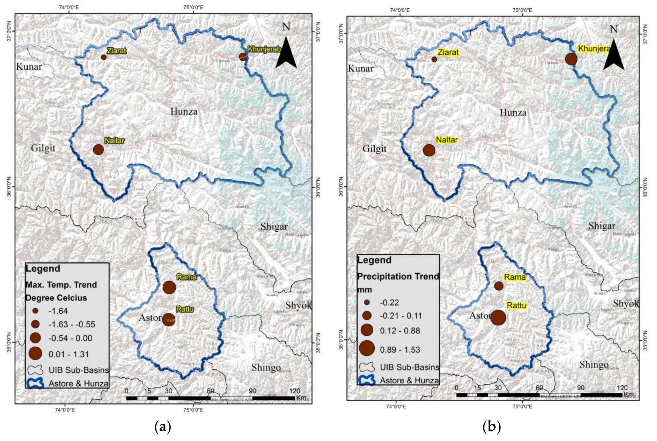
Spatial variations in the mean annual maximum temperature and precipitation trends were analyzed for the Hunza and the Astore River basins in ArcGIS. The results showed that there is a decreasing trend in mean annual maximum temperature in Hunza, whereas for Astore it is increasing (Figure 4a). This increase in temperature causes the snow and ice melting in Astore, and hence increases the Astore River discharge. Similarly, Figure 4b represents the spatial variation in the increasing trend in precipitation for both basins. However, it is the solid precipitation (snow) which causes the nourishment and advancement of glaciers at high altitude in the Hunza basin. On the other hand, the increase in liquid precipitation (rainfall) is due to the influence of the monsoon system in the Astore basin. This increase in precipitation also accelerates the discharge in the Astore river system. Similar findings were also reported by Tahir et al. [10] and Hassan et al. [1]. This spatial variability in both temperature and precipitation can mainly be attributed to variation in the topography and aspect of the Hunza and Astore basins.
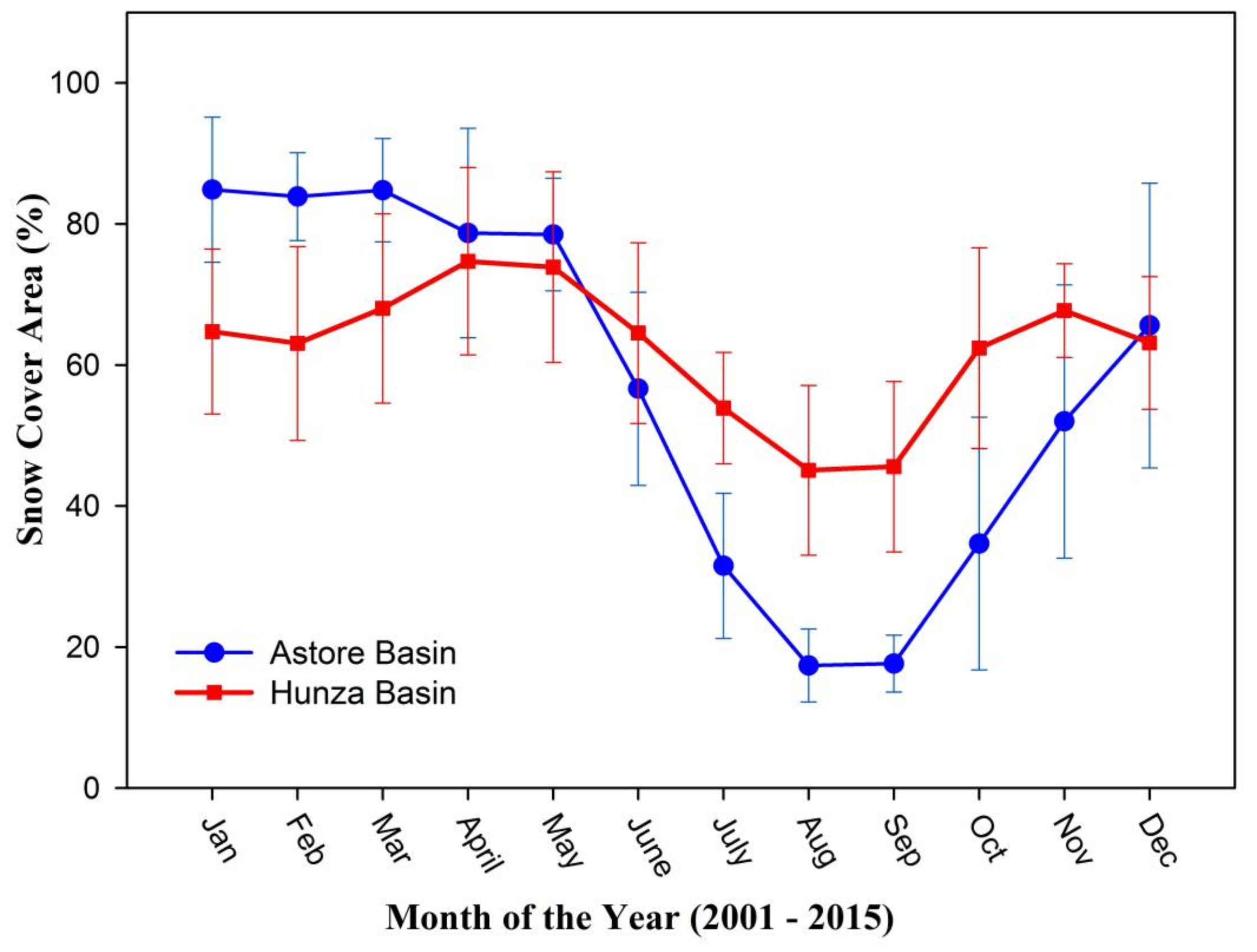
3.2. Spatial Variability Analysis of Snow Cover of the Hunza and Astore Sub-Basins
Snow cover areas of the Hunza and Astore basins were spatially analyzed using MODIS satellite imagery of 8 day-interval over a period of 15 years. The average snow cover of the Astore basin varies from about 92% in winter to 15% in summer (Figure 5). Whereas, Hunza snow cover varies from about 75% in winter to 50% in summer over a 15-year period. As Astore is a low altitude basin, the snow accumulation period starts in October and the maximum snow cover reaches around 90–92% in March (Figure 5). In contrast, Hunza is a high altitude basin which is dominated by the westerly system, and the snow accumulation starts in September and reaches its maximum extent (75–80%) in April. In the Astore basin the snowmelt period starts in late April and the minimum snow cover is observed during August and September when the snow cover drops to 10–15% (Figure 5).
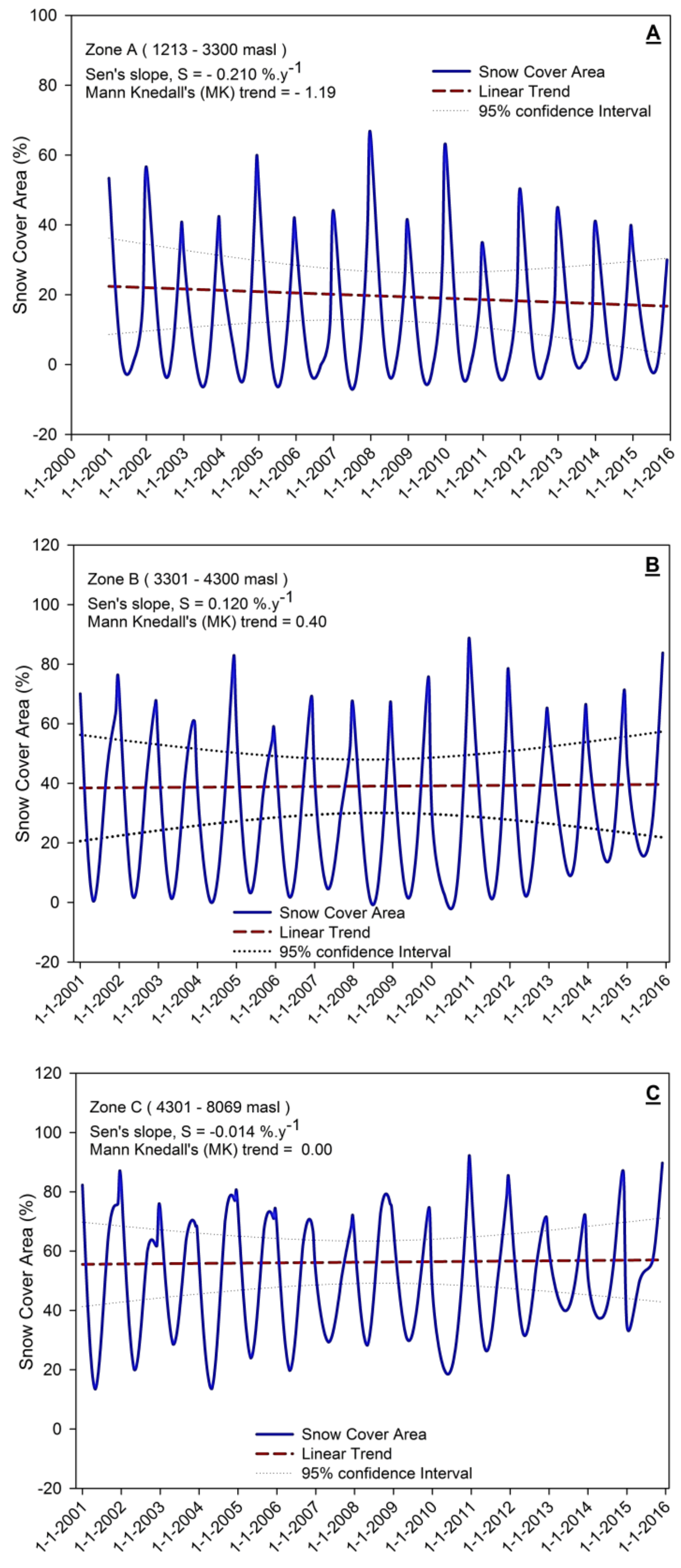
To assess the impact of climate change on snow cover at different altitudes of the UIB, the Astore and Hunza sub-basins were divided into three elevation zones (Table 1). The Astore basin zone A covered about 16% (i.e., the lowest elevation zone 1213–3300 m) of the total area of the catchment and the precipitation in this zone is mostly in the form of rainfall. Due to an increase in maximum temperature in zone A, the snow cover trend was found to be decreasing with Mann-Kendall value of Z = −0.21 and Sen’s slope = −1.19% year−1 (Figure 6). Zone B covers approximately 50% (i.e., the middle elevation class 3301–4300 m) of the total area of the Astore catchment and receives a large proportion of the precipitation in the form of snowfall (Figure 2; Table 1). As it represents almost 50% of the basin and is mostly fed by snowfall, this zone has a strong tendency to influence the runoff in the basin, whereas the snow cover trend was found to be non-significant in zone B (Z = 0.4; Sen’s slope = 0.12% year−1). However, if the temperature at this elevation zone increased in future as projected by the trend identified in this study, then it will significantly affect the basin’s hydrology, i.e., more snowmelt will generate higher runoff over time. Zone C covers about 34% (i.e., the highest elevation class, 4301–8069 m) of the total area of the Astore catchment and it is largely covered with glaciers, especially above 5000 m (Figure 6). A slightly increasing or almost stable snow cover trend was observed in this zone (Z = 0.001; Sen’s slope = 0.014% year−1).
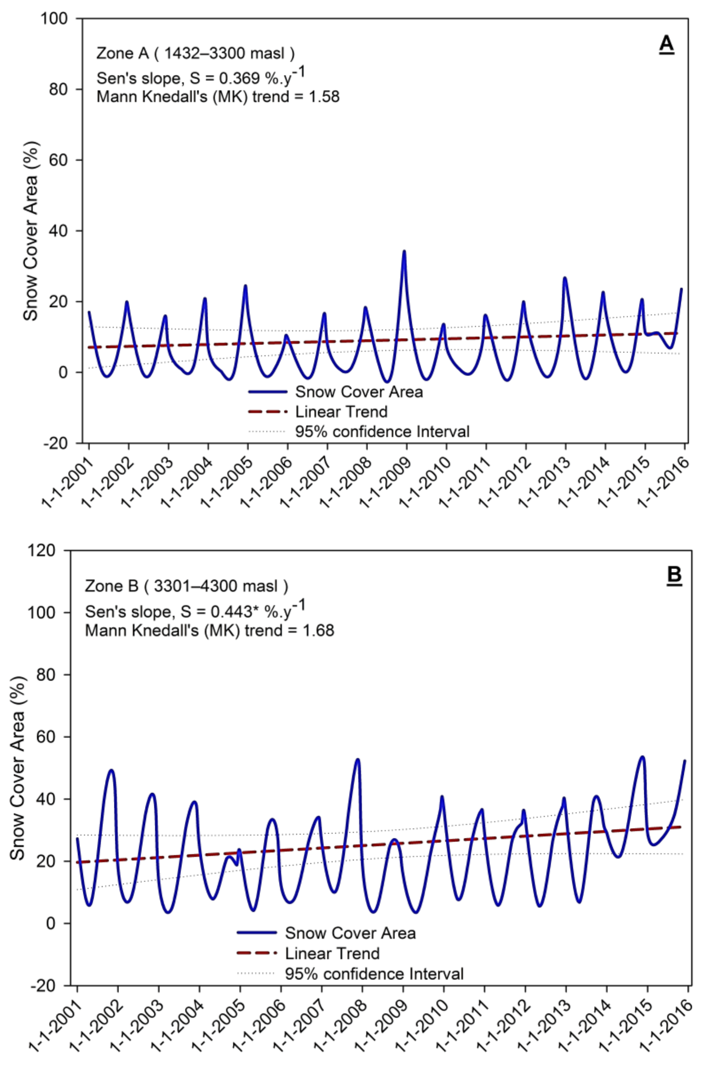
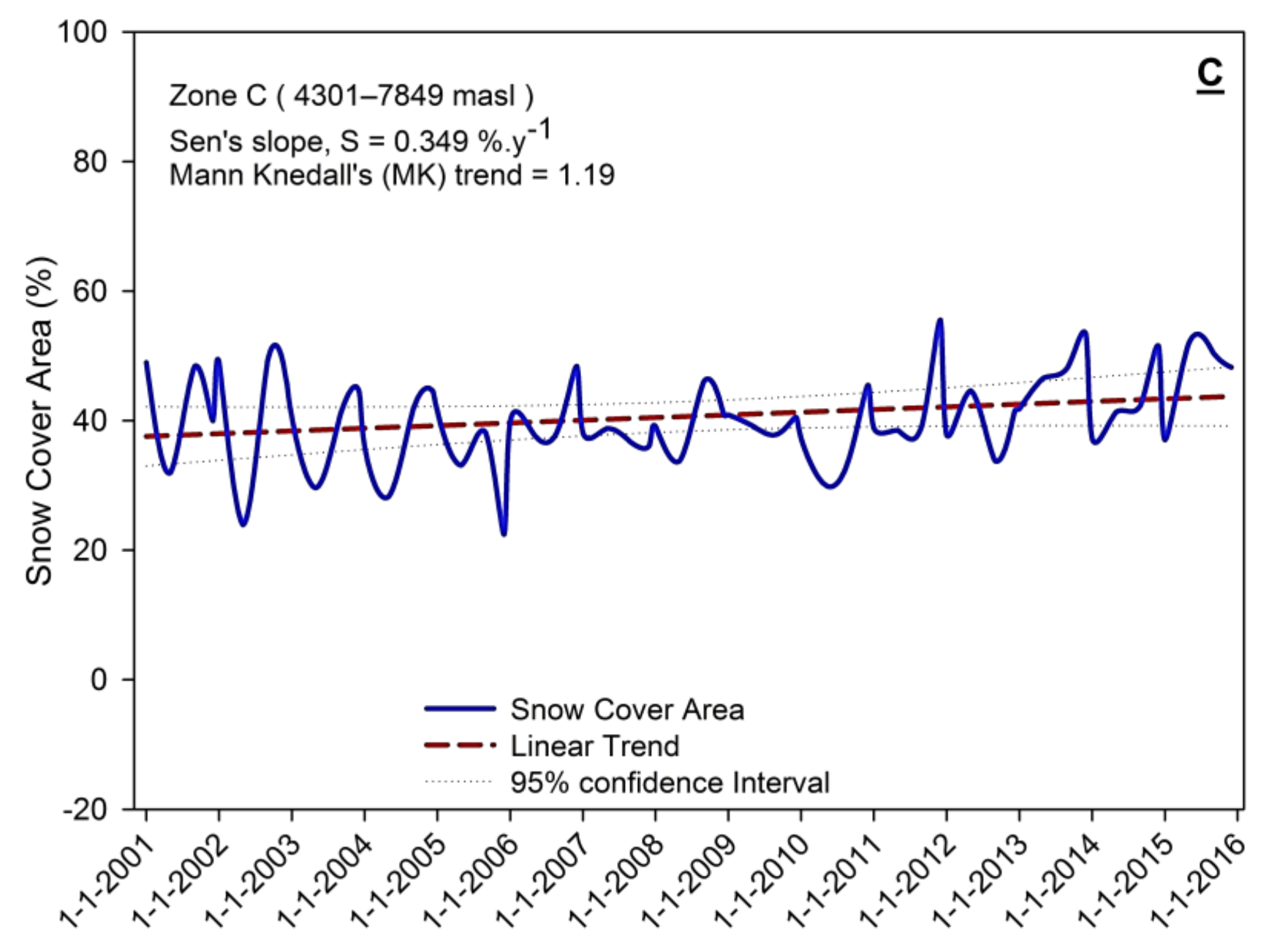
In the Hunza basin, the snow cover trend was slightly different in zone A (11% coverage) than the Astore basin. A non-significant increasing snow cover trend (Z = 1.58 and Sen’s slope = 0.369% year−1) was observed in zone A of the Hunza basin which could also be described as stable, whereas a slightly increasing snow cover trend was found in zones B and C of the Hunza basin. A Kendall tau (Z) coefficient value of Z = 0.44 and a Sen’s slope value of 1.68% year−1 was found in Zone B (25% area coverage) of the Hunza River basin (Figure 7), while the trend value Z = 0.34 with a Sen’s slope of 1.19% year−1 was found in Zone C (64% area coverage) of the Hunza River basin. The stable (or slightly increasing) trends of the snow cover in zones A, B and C of the Hunza basin are mainly responsible for the overall consistently increasing trend in the snow cover area in the catchment. About 98% of the area of the Hunza basin lies above an elevation of 2000 m and about 32.5% of the Hunza basin area is located above 5000 m where the temperature remains well below freezing throughout the year, and which receives comparatively more snow due to the westerly system at this altitude. This could be the reason for the slight increase in snow cover and advancement of some glaciers in the Hunza basin.
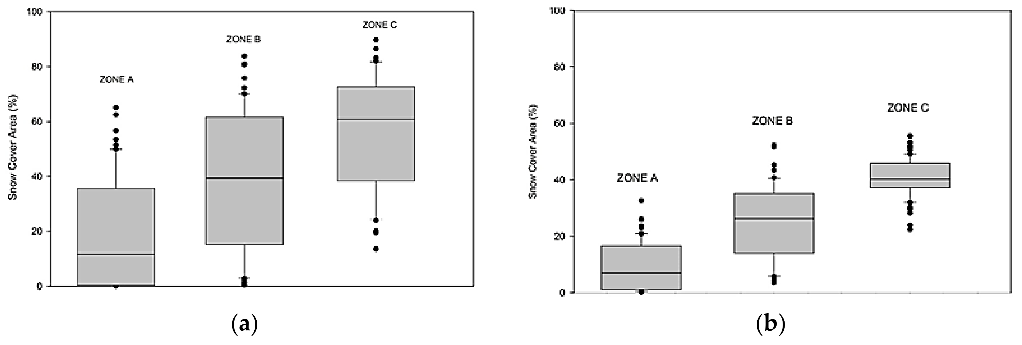
The Astore basin shows higher interannual variability in the extent of snow cover than the Hunza basin in different elevation zones (Figure 8). For example, the Astore basin shows snow cover variations for zone A ranging from 0% to 38%, 15% to 60% in zone B, and 38% to 65% in zone C. While, the Hunza basin shows comparatively less variability in snow cover area, i.e., from 2% to 18% in zone A, 16% to 35% in zone B and 38% to 43% in zone C.
4. Conclusions
This study analyzed the climatic variables of two contrasting sub-basins of the UIB (Hunza and Astore) regarding trends in temperature, precipitation, discharge and snow cover using the non-parametric Mann-Kendall and Sen’s slope estimator. In the Astore sub-basin, the river discharge and precipitation were significantly (p ≤ 0.05) increased with a Sen’s slope value of 1.039 m3·s−1·year−1 and 0.192 mm·year−1, respectively, while the temperature was non-significantly (p ≥ 0.05) increased with the Sen’s slope value of 0.041 °C·year−1. On the other hand, in the Hunza sub-basin, the river discharge and temperature significantly (p ≤ 0.05) decreased with a Sen’s slope value of −2.541 m3·s−1·year−1 and −0.034 °C·year−1, respectively, while precipitation showed a non-significant (p ≥ 0.05) increasing trend with a Sen’s slope value of 0.023 mm·year−1. It can be argued that the temperature declining trend and higher amount of solid precipitation due to the strong influence of westerly system, resulted in a decline in discharge in the Hunza sub-basin. In comparison, the Astore sub-basin, which is strongly influenced by the monsoon system, experienced an increasing trend in liquid precipitation and higher temperature due to its lower altitude resulting in an increasing trend in discharge. The snow cover analysis results suggest that the Western Himalayas (Astore basin) and Central Karakoram region (Hunza River basin) of the UIB had a stable and slightly increasing trend in snow cover with a Sen’s slope of 0.07% year−1 and 0.394% year−1, respectively. The study compared the contrasting hydrometeorological trends in the sub-basins of the upper Indus basin which helps to understand the Karakorum anomaly, i.e., the behavior of glaciers in the Karakoram region where some glaciers are surging instead of retreating. Based on the results of this study it can be concluded that since both sub-basins are influenced by different climatological systems (monsoon and westerly), the results of those studies where the Upper Indus basin is treated as one unit in hydrometeorological modeling should be used with caution. Further studies should be conducted to assess the impact of climate change on the water resources of the UIB at sub-basin level under climate change scenarios. This study may help water resource managers, agricultural planners and decision makers to obtain better insight into the effects of climate variability on water resources of UIB.
Author Contributions
Iqra Atif is the main contributor to this work and conducted the research, performed the statistical analysis and manuscript writing under the supervision of Javed Iqbal, Associate Professor and Head of Department, who extensively reviewed the manuscript and writing the manuscript. Muhammad Ahsan Mahboob, Assistant Professor IGIS-NUST, significantly contributed to data analysis and manuscript writing.
Funding
This research received no external funding.
Acknowledgments
This study acknowledges contributions from the Water and Power Development Authority (WAPDA) for providing hydrometeorological data and National Aeronautics and Space Administration (NASA) for making free availability of MODIS data. The constructive feedback from anonymous reviewers has also helped to improve the manuscript. The views articulated here are solely of the author and are not necessarily a reflection of the aforementioned organizations.
Conflicts of Interest
The authors declare no conflict of interest.
Appendix A
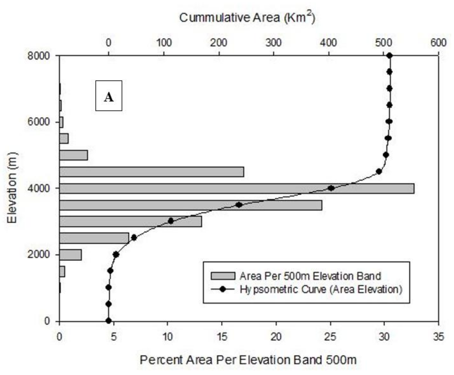
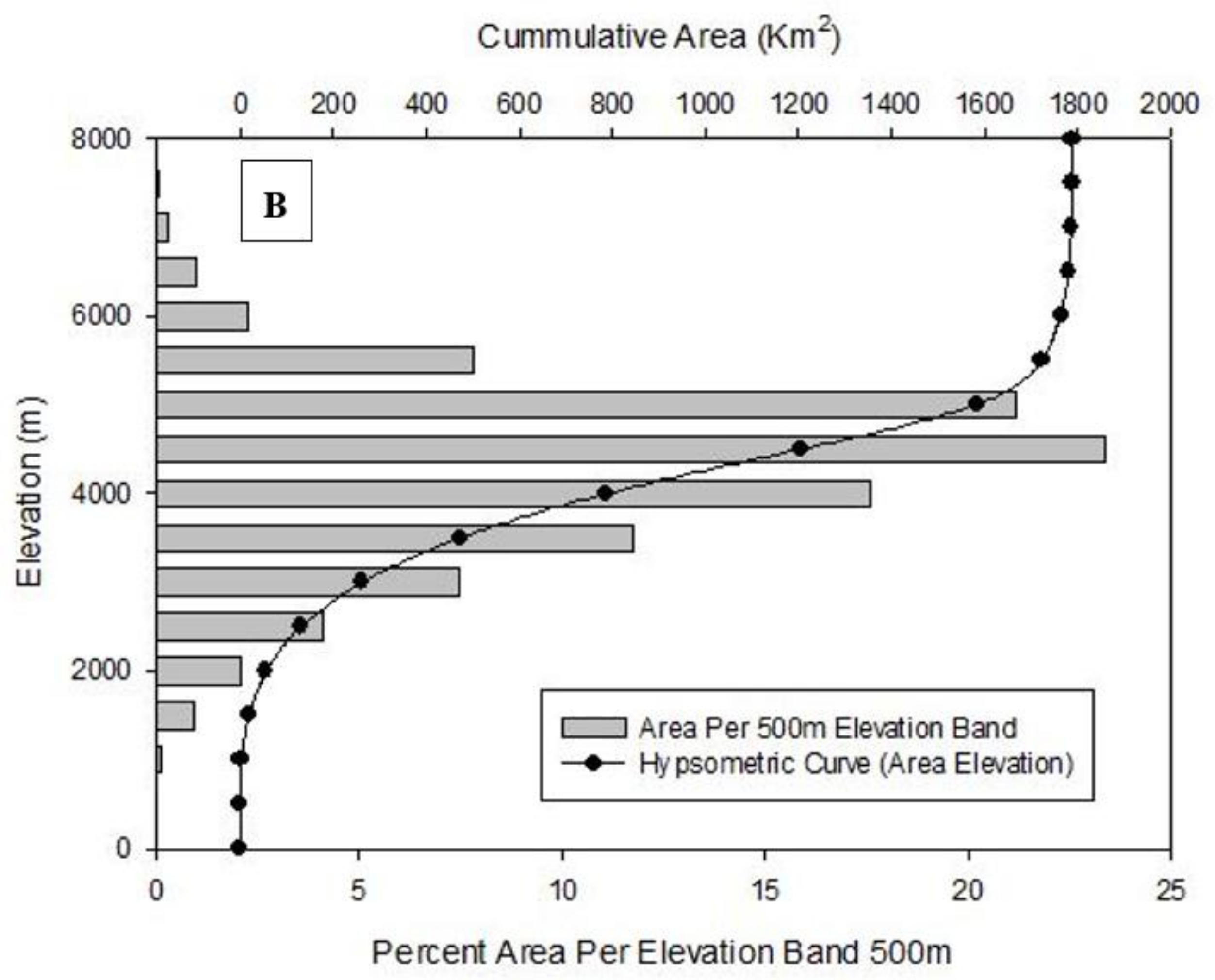
Hypsometric curves of the cumulative distribution function of elevations of Astore (A) and Hunza (B) sub-basins.
Figure A1.
Hypsometric curve of Astore (A) and Hunza (B) sub-basins.


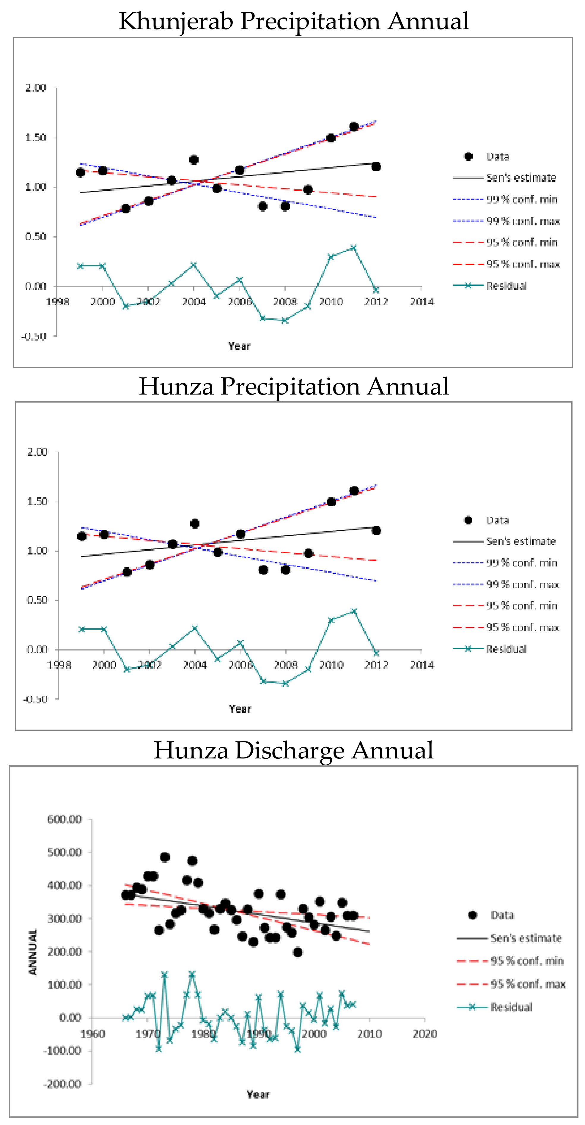
Appendix B
Sen’s slope estimation and Trend analysis of Hunza Basin hydrometeorological parameters at 99% and 95% confidence interval with residuals.
Figure A2.
Hunza sub-basin’s hydrometeorological trends of different stations.


Appendix C
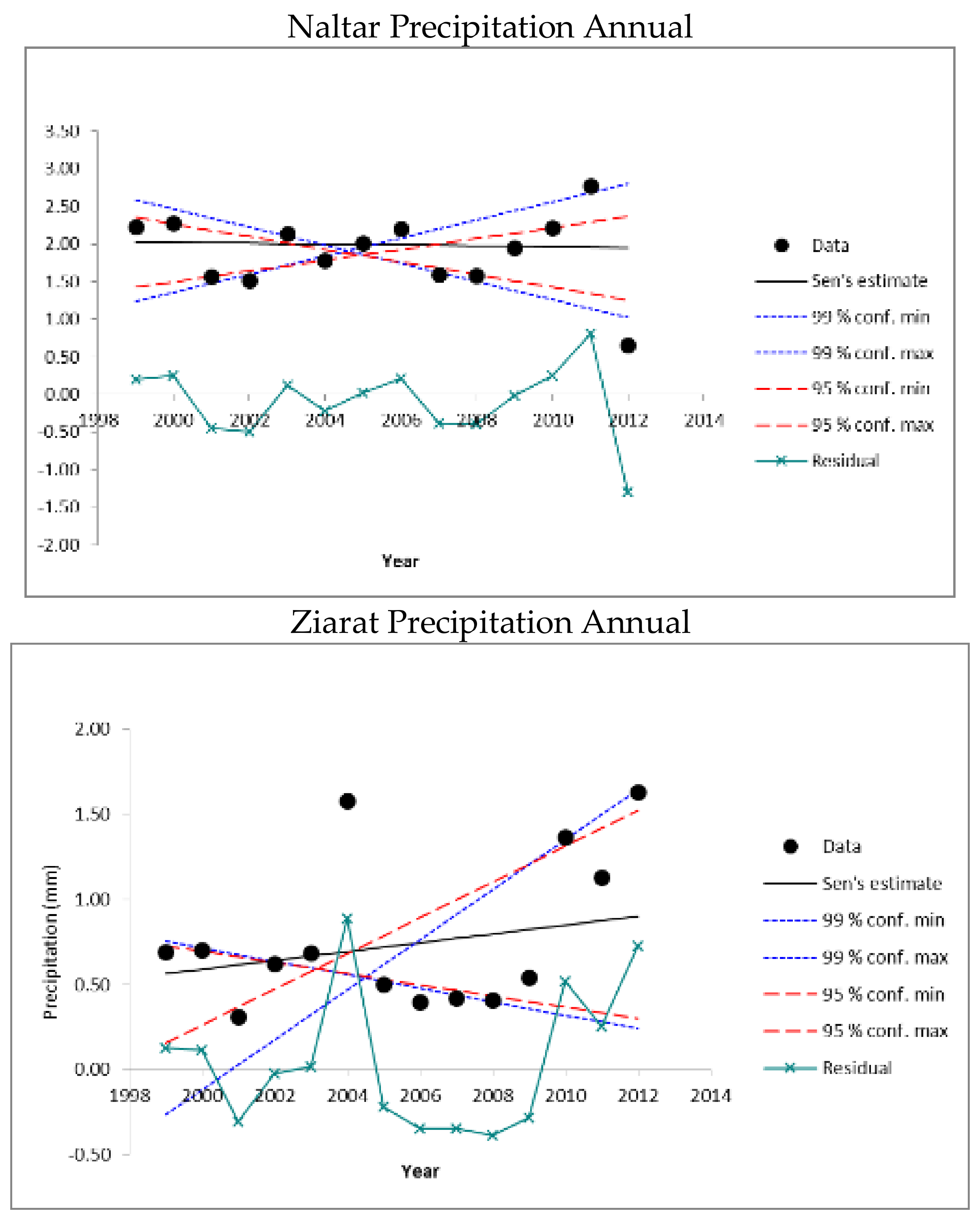
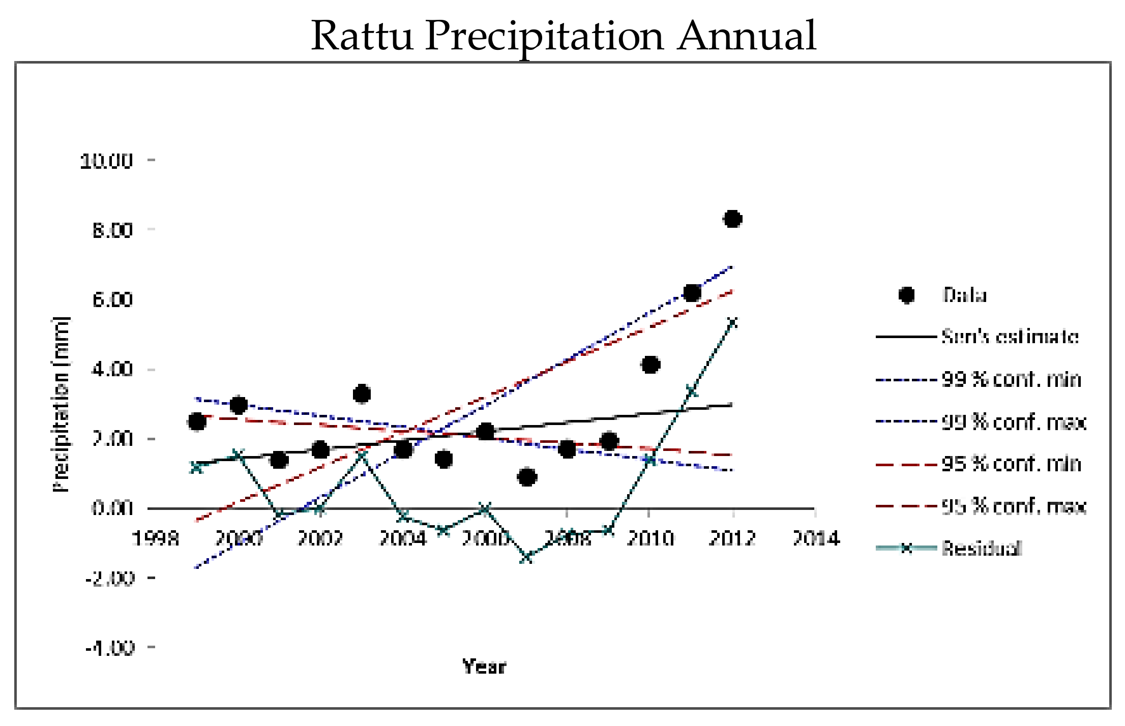
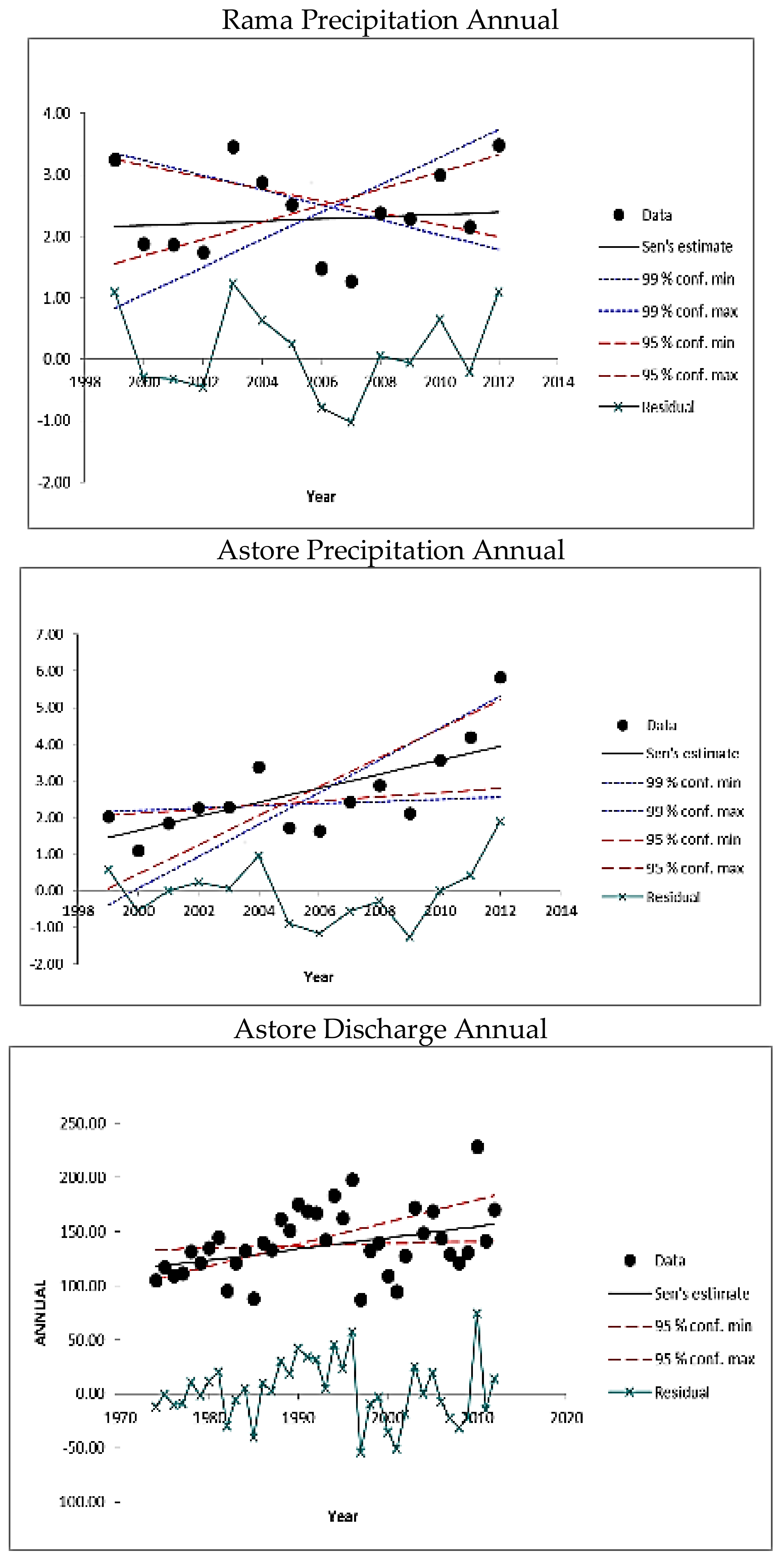
Sen’s slope estimation and trend analysis of Astore Basin precipitation at 99% and 95% confidence interval with residuals.
Figure A3.
Astore sub-basin’s hydrometeorological trends of different stations.


References
- Hassan, J.; Kayastha, R.B.; Shrestha, A.; Bano, I.; Ali, S.H.; Magsi, H.Z. Predictions of future hydrological conditions and contribution of snow and ice melt in total discharge of Shigar River Basin in Central Karakoram, Pakistan. Sci. Cold Arid Reg. 2017, 9, 511–524. [Google Scholar]
- Tahir, A.A.; Chevallier, P.; Arnaud, Y.; Neppel, L.; Ahmad, B. Modeling snowmelt-runoff under climate scenarios in the Hunza River basin, Karakoram Range, Northern Pakistan. J. Hydrol. 2011, 409, 104–117. [Google Scholar] [CrossRef]
- Hewitt, K. The Karakoram anomaly? Glacier expansion and the ‘elevation effect’, Karakoram Himalaya. Mount. Res. Dev. 2005, 25, 332–340. [Google Scholar] [CrossRef]
- Hewitt, K. Tributary glacier surges: An exceptional concentration at Panmah Glacier, Karakoram Himalaya. J. Glaciol. 2007, 53, 181–188. [Google Scholar] [CrossRef]
- Archer, D. Contrasting hydrological regimes in the upper Indus Basin. J. Hydrol. 2003, 274, 198–210. [Google Scholar] [CrossRef]
- Forsythe, N.; Kilsby, C.G.; Fowler, H.J.; Archer, D.R. Assessment of runoff sensitivity in the Upper Indus Basin to interannual climate variability and potential change using MODIS satellite data products. Mount. Res. Dev. 2012, 32, 16–29. [Google Scholar] [CrossRef]
- Winiger, M.; Gumpert, M.; Yamout, H. Karakorum–Hindukush–western Himalaya: Assessing high-altitude water resources. Hydrol. Process. 2005, 19, 2329–2338. [Google Scholar] [CrossRef]
- Wake, C.P. Glaciochemical investigations as a tool for determining the spatial and seasonal variation of snow accumulation in the central Karakoram, northern Pakistan. Ann. Glaciol. 1989, 13, 279–284. [Google Scholar] [CrossRef]
- Immerzeel, W.; Wanders, N.; Lutz, A.; Shea, J.; Bierkens, M. Reconciling high-altitude precipitation in the upper Indus basin with glacier mass balances and runoff. Hydrol. Earth Syst. Sci. 2015, 19, 4673–4687. [Google Scholar] [CrossRef]
- Tahir, A.A.; Adamowski, J.F.; Chevallier, P.; Haq, A.U.; Terzago, S. Comparative assessment of spatiotemporal snow cover changes and hydrological behavior of the Gilgit, Astore and Hunza River basins (Hindukush–Karakoram–Himalaya region, Pakistan). Meteorol. Atmos. Phys. 2016, 128, 793–811. [Google Scholar] [CrossRef]
- Fleming, S.W.; Hood, E.; Dahlke, H.; O’Neel, S. Seasonal flows of international British Columbia-Alaska rivers: The nonlinear influence of ocean-atmosphere circulation patterns. Adv. Water Resour. 2016, 87, 42–55. [Google Scholar] [CrossRef]
- Van Wilgen, N.J.; Goodall, V.; Holness, S.; Chown, S.L.; McGeoch, M.A. Rising temperatures and changing rainfall patterns in South Africa’s national parks. Int. J. Climatol. 2016, 36, 706–721. [Google Scholar] [CrossRef]
- Sharma, C.S.; Panda, S.N.; Pradhan, R.P.; Singh, A.; Kawamura, A. Precipitation and temperature changes in eastern India by multiple trend detection methods. Atmos. Res. 2016, 180, 211–225. [Google Scholar] [CrossRef]
- Fowler, H.; Archer, D. Conflicting signals of climatic change in the Upper Indus Basin. J. Clim. 2006, 19, 4276–4293. [Google Scholar] [CrossRef]
- Bocchiola, D.; Diolaiuti, G. Recent (1980–2009) evidence of climate change in the upper Karakoram, Pakistan. Theor. Appl. Climatol. 2013, 113, 611–641. [Google Scholar] [CrossRef]
- Kunkel, K.E.; Karl, T.R.; Brooks, H.; Kossin, J.; Lawrimore, J.H.; Arndt, D.; Bosart, L.; Changnon, D.; Cutter, S.L.; Doesken, N. Monitoring and understanding trends in extreme storms: State of knowledge. Bull. Am. Meteorol. Soc. 2013, 94, 499–514. [Google Scholar] [CrossRef]
- Blain, G.C. The influence of nonlinear trends on the power of the trend-free pre-whitening approach. Acta Sci. Agron. 2015, 37, 21–28. [Google Scholar] [CrossRef]
- Forkel, M.; Carvalhais, N.; Verbesselt, J.; Mahecha, M.D.; Neigh, C.S.; Reichstein, M. Trend change detection in NDVI time series: Effects of inter-annual variability and methodology. Remote Sens. 2013, 5, 2113–2144. [Google Scholar] [CrossRef]
- Bhutiyani, M.R. Climate change in the Northwestern Himalayas. In Dynamics of Climate Change and Water Resources of Northwestern Himalaya; Springer: Cham, Switzerland, 2015; pp. 85–96. [Google Scholar]
- Panthi, J.; Dahal, P.; Shrestha, M.L.; Aryal, S.; Krakauer, N.Y.; Pradhanang, S.M.; Lakhankar, T.; Jha, A.K.; Sharma, M.; Karki, R. Spatial and temporal variability of rainfall in the Gandaki River Basin of Nepal Himalaya. Climate 2015, 3, 210–226. [Google Scholar] [CrossRef]
- Sen, P.K. Estimates of the regression coefficient based on Kendall’s tau. J. Am. Stat. Assoc. 1968, 63, 1379–1389. [Google Scholar] [CrossRef]
- Zarei, A.R.; Moghimi, M.M.; Mahmoudi, M.R. Parametric and Non-Parametric Trend of Drought in Arid and Semi-Arid Regions Using RDI Index. Water Resour. Manag. 2016, 30, 5479–5500. [Google Scholar] [CrossRef]
- Cohen, J.; Cohen, P.; West, S.G.; Aiken, L.S. Applied Multiple Regression/Correlation Analysis for the Behavioral Sciences; Routledge: Abingdon, UK, 2013. [Google Scholar]
- Jain, S.K.; Kumar, V. Trend analysis of rainfall and temperature data for India. Curr. Sci. 2012, 102, 37–49. [Google Scholar]
- Salmi, M.; Auslender, F.; Bornert, M.; Fogli, M. Various estimates of Representative Volume Element sizes based on a statistical analysis of the apparent behavior of random linear composites. C. R. Méc. 2012, 340, 230–246. [Google Scholar] [CrossRef]
- Chaudhuri, S.; Dutta, D. Mann–kendall trend of pollutants, temperature and humidity over an urban station of India with forecast verification using different arima models. Environ. Monit. Assess. 2014, 186, 4719–4742. [Google Scholar] [CrossRef] [PubMed]
- Drápela, K.; Drápelová, I. Application of mann-kendall test and the Sen’s slope estimates for trend detection in deposition data from Bílý Kříž (Beskydy Mts., the Czech Republic) 1997–2010. Beskydy 2011, 4, 133–146. [Google Scholar]
- Kumar, R.; Farooq, Z.; Jhajharia, D.; Singh, V. Trends in temperature for the Himalayan environment of Leh (Jammu and Kashmir), India. In Climate Change Impacts; Springer: Singapore, 2018; pp. 3–13. [Google Scholar]
- Liu, X.; Zhu, X.; Pan, Y.; Li, S.; Ma, Y.; Nie, J. Vegetation dynamics in qinling-daba mountains in relation to climate factors between 2000 and 2014. J. Geogr. Sci. 2016, 26, 45–58. [Google Scholar] [CrossRef]
- Saavedra, F.A.; Kampf, S.K.; Fassnacht, S.R.; Sibold, J.S. Changes in ANDES snow cover from MODIS data, 2000–2016. Cryosphere 2018, 12, 1027–1046. [Google Scholar] [CrossRef]
- Sirguey, P.; Mathieu, R.; Arnaud, Y. Subpixel monitoring of the seasonal snow cover with MODIS at 250 m spatial resolution in the Southern Alps of New Zealand: Methodology and accuracy assessment. Remote Sens. Environ. 2009, 113, 160–181. [Google Scholar] [CrossRef]
- Atif, I.; Mahboob, M.A.; Iqbal, J. Snow cover area change assessment in 2003 and 2013 using MODIS data of the Upper Indus Basin, Pakistan. J. Himal. Earth Sci. 2015, 48, 117–128. [Google Scholar]
- Cheema, M.J.M.; Bastiaanssen, W.G. Local calibration of remotely sensed rainfall from the trmm satellite for different periods and spatial scales in the indus basin. Int. J. Remote Sens. 2012, 33, 2603–2627. [Google Scholar] [CrossRef]
- Hewitt, K.; Wake, C.P.; Young, G.; David, C. Hydrological investigations at Biafo Glacier, Karakoram Range, Himalaya; an important source of water for the Indus River. Ann. Glaciol. 1989, 13, 103–108. [Google Scholar] [CrossRef]
- Lal, R. Soil carbon sequestration impacts on global climate change and food security. Science 2004, 304, 1623–1627. [Google Scholar] [CrossRef] [PubMed]
- Førland, E.; Allerup, P.; Dahlström, B.; Elomaa, E.; Jónsson, T.; Madsen, H.; Perälä, J.; Rissanen, P.; Vedin, H.; Vejen, F. Manual for operational correction of Nordic precipitation data. DNMI Rep. 1996, 24, 96. [Google Scholar]
- Hall, D.K.; Riggs, G.A.; Salomonson, V.V.; DiGirolamo, N.E.; Bayr, K.J. Modis snow-cover products. Remote Sens. Environ. 2002, 83, 181–194. [Google Scholar] [CrossRef]
- Wang, X.; Xie, H.; Liang, T. Evaluation of MODIS snow cover and cloud mask and its application in northern Xinjiang, China. Remote Sens. Environ. 2008, 112, 1497–1513. [Google Scholar] [CrossRef]
- Liu, J.; Zhang, W.; Liu, T. Monitoring recent changes in snow cover in central Asia using improved MODIS snow-cover products. J. Arid Land 2017, 9, 763–777. [Google Scholar] [CrossRef]
- Chen, Y.; Huang, C.; Ticehurst, C.; Merrin, L.; Thew, P. An evaluation of MODIS daily and 8-day composite products for floodplain and wetland inundation mapping. Wetlands 2013, 33, 823–835. [Google Scholar] [CrossRef]
- Hasson, S.; Böhner, J.; Lucarini, V. Prevailing climatic trends and runoff response from Hindukush–Karakoram–Himalaya, Upper Indus Basin. Earth Syst. Dyn. 2017, 8, 337–355. [Google Scholar] [CrossRef]
- Tahir, A.A.; Chevallier, P.; Arnaud, Y.; Ashraf, M.; Bhatti, M.T. Snow cover trend and hydrological characteristics of the Astore River basin (Western Himalayas) and its comparison to the Hunza basin (Karakoram region). Sci. Total Environ. 2015, 505, 748–761. [Google Scholar] [CrossRef] [PubMed]
- Kang, H.M.; Yusof, F. Homogeneity tests on daily rainfall series. Int. J. Contemp. Math. Sci. 2012, 7, 9–22. [Google Scholar]
- Von Storch, H. Misuses of statistical analysis in climate research. In Analysis of Climate Variability; Springer: Berlin, Germany, 1999; pp. 11–26. [Google Scholar]
- Yue, S.; Wang, C.Y. Applicability of Prewhitening to eliminate the influence of serial correlation on the Mann-Kendall test. Water Resour. Res. 2002, 38, 1068. [Google Scholar] [CrossRef]
- Minitab 18 Statistical Software [Computer Software]; State College PM, Inc.: State College, PA, USA, 2018.
- Barua, S.; Muttil, N.; Ng, A.; Perera, B. Rainfall trend and its implications for water resource management within the Yarra River catchment, Australia. Hydrol. Process. 2013, 27, 1727–1738. [Google Scholar] [CrossRef]
- Dawood, M. Spatio-statistical analysis of temperature fluctuation using Mann–Kendall and Sen’s slope approach. Clim. Dyn. 2017, 48, 783–797. [Google Scholar]
- Hussain, S.S.; Mudasser, M.; Sheikh, M.; Manzoor, N. Climate change and variability in mountain regions of Pakistan implications for water and agriculture. Pak. J. Meteorol. 2005, 2, 75–90. [Google Scholar]
- Scherler, D.; Bookhagen, B.; Strecker, M.R. Spatially variable response of Himalayan glaciers to climate change affected by debris cover. Nat. Geosci. 2011, 4, 156–159. [Google Scholar] [CrossRef]
- Archer, D.R.; Fowler, H.J. Spatial and temporal variations in precipitation in the Upper Indus Basin, global teleconnections and hydrological implications. Hydrol. Earth Syst. Sci. Discuss. 2004, 8, 47–61. [Google Scholar] [CrossRef]
- Oouchi, K.; Noda, A.T.; Satoh, M.; Wang, B.; Xie, S.P.; Takahashi, H.G.; Yasunari, T. Asian summer monsoon simulated by a global cloud-system-resolving model: Diurnal to intra-seasonal variability. Geophys. Res. Lett. 2009, 36, 269–271. [Google Scholar] [CrossRef]
- Tiwari, S.; Kar, S.C.; Bhatla, R. Atmospheric moisture budget during winter seasons in the western himalayan region. Clim. Dyn. 2017, 48, 1277–1295. [Google Scholar] [CrossRef]
- Chevallier, P.; Arnaud, Y.; Ahmad, B. Snow cover dynamics and hydrological regime of the Hunza River basin, Karakoram Range, Northern Pakistan. Hydrol. Earth Syst. Sci. 2011, 15, 2259–2274. [Google Scholar]
- Ahmad, I.; Tang, D.; Wang, T.; Wang, M.; Wagan, B. Precipitation trends over time using Mann-Kendall and spearman’s rho tests in Swat River Basin, Pakistan. Adv. Meteorol. 2015, 2015, 431860. [Google Scholar] [CrossRef]
Figure 1.
Map of the study area showing the Hunza and Astore sub-basins of the upper Indus Basin along with the glaciers. The glaciers’ boundaries were delineated from the LANDSAT 7 ETM+ using the Normalized Difference Index (NDSI), Slope, Aspect, Normalized Difference Vegetation Index (NDVI) and Land Water Mask (LWM) filters.

Figure 2.
Showing three altitudinal zones of the Hunza and Astore River basins extracted from Global Digital Elevation Model (GDEM) along with glacier coverage and gauging stations.
Figure 2.
Showing three altitudinal zones of the Hunza and Astore River basins extracted from Global Digital Elevation Model (GDEM) along with glacier coverage and gauging stations.

Figure 3.
Methodological flow chart of the research work.

Figure 4.
Shows the Mann-Kendall trend of meteorological variables, maximum temperature °C·year−1 and precipitation mm·year−1 in the Hunza and Astore basins. (a) Maximum temperature; (b) Precipitation.
Figure 4.
Shows the Mann-Kendall trend of meteorological variables, maximum temperature °C·year−1 and precipitation mm·year−1 in the Hunza and Astore basins. (a) Maximum temperature; (b) Precipitation.

Figure 5.
The annual cycle in snow-covered area as a percentage of the total area estimated through the analysis of MODIS snow images for 15 individual years (2001–2015) for the Astore and Hunza basins. The bars indicate standard deviation of snow cover for each month across the year.
Figure 5.
The annual cycle in snow-covered area as a percentage of the total area estimated through the analysis of MODIS snow images for 15 individual years (2001–2015) for the Astore and Hunza basins. The bars indicate standard deviation of snow cover for each month across the year.

Figure 6.
The trend of the MODIS-data derived snow-covered area of the Astore River basin, in three altitudinal zones shown in (A–C), over a 15-year period (2001–2015).
Figure 6.
The trend of the MODIS-data derived snow-covered area of the Astore River basin, in three altitudinal zones shown in (A–C), over a 15-year period (2001–2015).

Figure 7.
The trend of MODIS-data derived snow-covered area the Hunza River basin, in three altitudinal zones shown in (A–C), over a 15-year period (2001–2015).
Figure 7.
The trend of MODIS-data derived snow-covered area the Hunza River basin, in three altitudinal zones shown in (A–C), over a 15-year period (2001–2015).


Figure 8.
The box-plot shows the interannual variability in snow-covered area of the (a) Astore and (b) Hunza River basin, in three altitudinal zones over a 15-year period (2001–2015).
Figure 8.
The box-plot shows the interannual variability in snow-covered area of the (a) Astore and (b) Hunza River basin, in three altitudinal zones over a 15-year period (2001–2015).


Table 1.
Main features of the elevation zones extracted from the ASTER GDEM of the Astore River and Hunza River basins.
Table 1.
Main features of the elevation zones extracted from the ASTER GDEM of the Astore River and Hunza River basins.
| Zone | A (Low-Altitude Zone) | B (Mid-Altitude Zone) | C (High-Altitude Zone) | |||
|---|---|---|---|---|---|---|
| Basin | Astore | Hunza | Astore | Hunza | Astore | Hunza |
| Elevation band (m) | 1213–3300 | 1432–3300 | 3301–4300 | 3301–4300 | 4301–8069 | 4301–7849 |
| Mean elevation (m) | ~2950 | ~2850 | ~3910 | ~3850 | ~4600 | ~5000 |
| Median elevation (m) | ~2263 | ~2366 | ~3800 | ~3800 | ~6132 | ~6067 |
| Area (%) | 16 | 11 | 50 | 25 | 34 | 64 |
| Area (km2) | 638 | 1541 | 1995 | 3413 | 1357 | 8779 |
Table 2.
Showing the Mann-Kendall trend and Sen’s slope estimator on an annual and seasonal basis in the Hunza Basin. Sen’s slope temperature, precipitation and discharge are increasing or decreasing in °C·year−1, mm·year−1 and m3·s−1·year−1, respectively. Seasonal distribution for spring (March–May), summer (June–August), fall (September–October), and winter (December–February).
| Stations | Spring | Summer | Fall | Winter | Annual | ||
|---|---|---|---|---|---|---|---|
| Ziarat | Tmin | Trend | 0.71 ↑ | −0.82 ↓ | 0.38 ↑ | 1.20 ↑ | 0.99 ↑ |
| Sen’s Slope | 0.03 | −0.05 | 0.01 | 0.08 | 0.06 | ||
| Tmax | Trend | 0.71 ↑ | −0.49 ↓ | 0.05 ↑ | 0 | 0 | |
| Sen’s Slope | 0.032 | −0.049 | 0.002 | −0.016 | −0.008 | ||
| Tavg | Trend | 0.82 ↑ | −0.60 ↓ | 0.16 ↑ | 0.33 ↑ | 0.44 ↑ | |
| Sen’s Slope | 0.031 | −0.057 | 0.006 | 0.03 | 0.037 | ||
| Precipitation | Trend | 0.99 ↑ | 0.22 ↑ | −0.44 ↓ | 2.30 * ↑ | 0.77 ↑ | |
| Sen’s Slope | 0.032 | 0.006 | −0.008 | 0.133 | 0.026 | ||
| Naltar | Tmin | Trend | −1.04 ↓ | −0.82 ↓ | −2.25 ↓ | −1.86 ↓ | −2.30 * ↓ |
| Sen’s Slope | −0.066 | −0.044 | −0.155 | −0.135 | −0.144 | ||
| Tmax | Trend | −0.82 ↓ | −0.05 ↓ | −1.48 ↓ | −1.64 ↓ | −1.86 ↓ | |
| Sen’s Slope | −0.047 | −0.02 | −0.066 | −0.113 | −0.075 | ||
| Tavg | Trend | −1.04 ↓ | −1.59 ↓ | −2.14 * ↓ | −2.41 * ↓ | −2.08 * ↓ | |
| Sen’s Slope | −0.159 | −0.201 | −0.158 | −0.142 | −0.155 | ||
| Precipitation | Trend | −1.20 ↓ | 0.00 | −1.04 ↓ | 1.09 ↑ | −0.22 ↓ | |
| Sen’s Slope | −0.115 | −0.004 | −0.036 | 0.063 | −0.006 | ||
| Khunjerab | Tmin | Trend | 2.41 * ↑ | 1.20 ↑ | 0.55 ↑ | 1.20 ↑ | 2.41 * ↑ |
| Sen’s Slope | 0.273 | 0.084 | 0.019 | 0.111 | 0.145 | ||
| Tmax | Trend | 0.88 ↑ | 0.55 ↑ | 0.11 ↑ | −0.55 ↓ | 0.11 ↑ | |
| Sen’s Slope | 0.037 | 0.012 | 0.014 | −0.058 | 0.01 | ||
| Tavg | Trend | 2.52 * ↑ | 1.31 ↑ | 0.33 ↑ | 0.77 ↑ | 1.75 ↑ | |
| Sen’s Slope | 0.228 | 0.07 | 0.024 | 0.065 | 0.068 | ||
| Precipitation | Trend | 1.86 ↑ | −2.30 * ↓ | 0.33 ↑ | 1.86 ↑ | 0.88 ↑ | |
| Sen’s Slope | 0.03 | −0.036 | 0.005 | 0.055 | 0.011 | ||
| Danyour Bridge | Trend | 0.57 ↑ | −3.13 ** ↓ | −1.64 ↓ | −0.16 ↓ | −2.94 ** ↓ | |
| Discharge | Sen’s Slope | 0.121 | −10.148 | −0.81 | −0.011 | −2.541 | |
| Hunza River Basin (Overall Statistics) | Tavg | Trend | 0.44 ↑ | −1.09 ↓ | −1.09 ↓ | −0.44 ↓ | −0.77 ↓ |
| Sen’s Slope | 0.033 | −0.058 | −0.046 | −0.047 | −0.034 | ||
| Precipitation | Trend | −0.11 ↓ | −0.44 ↓ | −0.44 ↓ | 2.52 * ↑ | 1.09 ↑ | |
| Sen’s Slope | −0.012 | −0.014 | −0.009 | 0.103 | 0.023 |
†, * and ** indicate significance at α = 0.1, 0.05 and 0.01, respectively ↑ indicate increasing trend; ↓ indicate decreasing trend.
Table 3.
Shows the Mann-Kendall trend and Sen’s slope estimator on an annual and seasonal basis in Astore Basin. Sen’s slope temperature, precipitation and discharge are increasing or decreasing in °C·year−1, mm·year−1 and m3·s−1·year−1, respectively. Seasonal distribution for spring (March–May), summer (June–August), fall (September–October), and winter (December–February).
| Climatic Station | Spring | Summer | Fall | Winter | Annual | ||
|---|---|---|---|---|---|---|---|
| Rattu | Tmin | Trend | −0.55 ↓ | 0.11 ↑ | −0.11 ↓ | −0.11 ↓ | −1.09 ↓ |
| Sen’s Slope | −0.052 | 0.018 | −0.014 | −0.022 | −0.031 | ||
| Tmax | Trend | −0.88 ↓ | 0.99 ↑ | −0.44 ↓ | 1.31 ↑ | 1.86 + ↑ | |
| Sen’s Slope | −0.113 | 0.061 | −0.018 | 0.101 | 0.046 | ||
| Tavg | Trend | −0.99 ↓ | 0.88 ↑ | −0.22 ↓ | 0.77 ↑ | 1.09 ↑ | |
| Sen’s Slope | −0.061 | 0.052 | −0.007 | 0.068 | 0.032 | ||
| Precipitation | Trend | 1.09 ↑ | 1.42 ↑ | 0 | 1.20 ↑ | 1.53 ↑ | |
| Sen’s Slope | 0.133 | 0.118 | −0.018 | 0.219 | 0.128 | ||
| Rama | Tmin | Trend | −0.11 ↓ | 0.05 ↑ | 0.99 ↑ | −0.33 ↓ | 0.55 ↑ |
| Sen’s Slope | −0.017 | 0.014 | 0.05 | −0.044 | 0.008 | ||
| Tmax | Trend | −0.99 ↓ | 1.04 ↑ | 1.09 ↑ | 0.99 ↑ | 2.08 * ↑ | |
| Sen’s Slope | −0.096 | 0.026 | 0.065 | 0.102 | 0.081 | ||
| Tavg | Trend | −0.22 ↓ | 0.16 ↑ | 0 | 0.77 ↑ | 1.53 ↑ | |
| Sen’s Slope | −0.055 | 0.015 | 0.001 | 0.074 | 0.035 | ||
| Precipitation | Trend | −0.55 ↓ | −0.38 ↓ | 0.55 ↑ | 1.31 ↑ | 0.11 ↑ | |
| Sen’s Slope | −0.047 | −0.001 | 0.036 | 0.131 | 0.018 | ||
| Doyian | Discharge | Trend | 3.80 ** ↑ | 1.14 ↑ | 2.15 * ↑ | 2.03 * ↑ | 2.44 * ↑ |
| Bridge | Sen’s Slope | 1.506 | 1.312 | 0.708 | 0.208 | 1.039 | |
| Astore River Basin (Overall Statistics) | Tavg | Trend | −0.77 ↓ | 0.66 ↑ | 0.66 ↑ | 0.77 ↑ | 1.75 † ↑ |
| Sen’s Slope | −0.065 | 0.034 | 0.016 | 0.064 | 0.041 | ||
| Precipitation | Trend | 2.30 * ↑ | 2.85 ** ↑ | 3.07 ** ↑ | 0.99 ↑ | 2.74 ** ↑ | |
| Sen’s Slope | 0.268 | 0.103 | 0.243 | 0.103 | 0.192 |
†, * and ** indicate significance at α = 0.1, 0.05 and 0.01, respectively. ↑ indicate increasing trend; ↓ indicate decreasing trend.
© 2018 by the authors. Licensee MDPI, Basel, Switzerland. This article is an open access article distributed under the terms and conditions of the Creative Commons Attribution (CC BY) license (http://creativecommons.org/licenses/by/4.0/).
Share and Cite
MDPI and ACS Style
Atif, I.; Iqbal, J.; Mahboob, M.A. Investigating Snow Cover and Hydrometeorological Trends in Contrasting Hydrological Regimes of the Upper Indus Basin. Atmosphere 2018, 9, 162. https://doi.org/10.3390/atmos9050162
AMA Style
Atif I, Iqbal J, Mahboob MA. Investigating Snow Cover and Hydrometeorological Trends in Contrasting Hydrological Regimes of the Upper Indus Basin. Atmosphere. 2018; 9(5):162. https://doi.org/10.3390/atmos9050162
Chicago/Turabian StyleAtif, Iqra, Javed Iqbal, and Muhammad Ahsan Mahboob. 2018. "Investigating Snow Cover and Hydrometeorological Trends in Contrasting Hydrological Regimes of the Upper Indus Basin" Atmosphere 9, no. 5: 162. https://doi.org/10.3390/atmos9050162
Note that from the first issue of 2016, this journal uses article numbers instead of page numbers. See further details here.