Article

Climate Change Impacts on Natural Sulfur Production: Ocean Acidification and Community Shifts

1
Los Alamos National Laboratory, Los Alamos, NM 87545, USA
2
Pacific Northwest National Laboratory, Joint Global Change Research Institute, 5825 University Research Court, College Park, MD 20740, USA
3
Oak Ridge National Laboratory, Oak Ridge, TN 37830, USA
4
Department of Civil & Environmental Engineering, University of Tennessee, Knoxville, TN 37996, USA
*
Author to whom correspondence should be addressed.
Atmosphere 2018, 9(5), 167; https://doi.org/10.3390/atmos9050167
Submission received: 15 February 2018 / Revised: 6 April 2018 / Accepted: 25 April 2018 / Published: 1 May 2018
(This article belongs to the Special Issue Ocean Contributions to the Marine Boundary Layer Aerosol Budget)

Abstract

:
Utilizing the reduced-complexity model Hector, a regional scale analysis was conducted quantifying the possible effects climate change may have on dimethyl sulfide (DMS) emissions within the oceans. The investigation began with a review of the sulfur cycle in modern Earth system models. We then expanded the biogeochemical representation within Hector to include a natural ocean component while accounting for acidification and planktonic community shifts. The report presents results from both a latitudinal and a global perspective. This new approach highlights disparate outcomes which have been inadequately characterized via planetary averages in past publications. Our findings suggest that natural sulfur emissions (ESN) may exert a forcing up to 4 times that of the CO2 marine feedback, 0.62 and 0.15 Wm−2, respectively, and reverse the radiative forcing sign in low latitudes. Additionally, sensitivity tests were conducted to demonstrate the need for further examination of the DMS loop. Ultimately, the present work attempts to include dynamic ESN within reduced-complexity simulations of the sulfur cycle, illustrating its impact on the global radiative budget.

1. Introduction

Dimethyl sulfide (DMS, CH3SCH3) is a semi-volatile organic compound produced by several environmental sources, totaling 25–80 TgS in global emissions. Natural sulfur is produced from sources such as volcanoes, biomass burnings, and fumaroles, with the largest contribution coming from phytoplankton [1]. However, the production rates of DMS and its precursor—dimethylsulfoniopropionate (DMPS)—varies a great deal throughout various functional groups and environmental conditions. Marine ecosystems contribute 50–60% of natural sulfur emissions and dominate the sulfur cycle in the Southern Hemisphere [2]. Once released from the mixed layer, the gaseous precursor—DMS—is oxidized in the lower atmosphere, resulting in a series of products, including sulfur dioxide (SO2). The SO2 has a final reaction with HOx oxidants, concluding with sulfate aerosol particles [3]. The sulfur-containing droplets disperse incoming solar radiation and act as condensation nuclei for cloud seeding, modifying the global radiative budget both directly and indirectly [1]. The compound first gained notoriety within the scientific community for its role in the CLAW hypothesis (Charlson, Lovelock, Andreae, and Warren). Authors of this paper concluded that organosulfur might act to mitigate consequences of a warming climate [4]. However, following the publication, more in-depth model investigations have reported DMS feedback may act to accelerate the impact of climate change, leading to additional warming [3]. For a supplementary examination of the formation and influence of natural sulfur emissions, refer to Menzo, 2018 [5].
An exhaustive anthology of articles exists examining individual impacts of climate change on DMS production. Findings detailed by author—such as Six et al., 2013 (S13), Flombaum et al., 2013 (F13), Cameron-Smith et al., 2011, and others—have served as an invaluable foundation for the present work [6,7,8]. However, to the best of the authors’ knowledge, limited comprehensive syntheses have been attempted. This shortage of integrated information motivates our current analysis. The examination began by reviewing the modern portrayal of the sulfur cycle in the reduced climate model Hector. We then built upon the typical biological representation by constructing a dynamic component which accounts for acidification. Next, the location and abundance of several phytoplankton classes were cataloged using present and end of century (EOC) simulations. These values were directly interpreted to quantify dimethyl sulfide contributions from each group. The investigation concluded with a range of sensitivity tests verifying the need for further evaluation of DMS in the global climate system.
In addition to bringing together the disparate effects of climate change on the phytoplankton community, this publication examines changes on a regional scale. We have partitioned global data into three meridional zones: northern high latitude (NHL), low latitude (LL), and southern high latitude (SHL). The segregation of information illustrates the diverse repercussions climate change can have on each section and the consequent influence on natural sulfur emissions (ESN). Ultimately, a localized approach attempts to calculate the varying impact that mounting carbon pollution has on natural sulfur production and, in turn, its influence on the radiative budget. This marine biogeochemical (mBGC) feedback is then contrasted with the familiar greenhouse gas equivalent—anthropogenic carbon dioxide (CO2)-and its role as a forcing agent.

2. Experiments

Our exploration is built upon the modern representation of the sulfur cycle within climate simulations. The Joint Global Change Research Institute (JGCRI) reduced-complexity model Hector was utilized due to its nearly instantaneous rendering-time and comprehensive format, which keeps each section separate and easy to manipulate. The model includes a one-pool atmosphere, land, and ocean component. The ocean is divided into a high- and low-latitude surface, an intermediate, and a deep box. Carbon first enters the high-latitude box and sinks to its depth. It then returns through the intermediate to the low-latitude surface box, simulating a simple thermohaline circulation. In its current state, Hector matches both historical trends and future projections comparable to observations and models included in the most recent Coupled Model Intercomparison Project. Hector is an open source platform and allows for the addition of new components. This duality provided an ideal opportunity to parameterize natural sulfur emissions and evaluate the output decisively. For a more detail description of Hector, refer to Hartin et al., 2015 [9]. The simple climate model (SCM) includes both a direct and an indirect sulfate aerosol equation (SOx). Considering the prime objective of the present work is to streamline dominant effects of ESN, we focused on the latter. The formula employed in Hector was adopted from Joos et al., 2001a [10]:
RF SO X Indirect = 0.6 × ( l n E S N + E S O x t E S N ) · ( l n E S N + E S O x t 0 E S N ) 1
The calculation requires a fixed input rate for ESN, anthropogenic sulfur emission during the year 2000 ( E S O x t 0 ), and a time series of man-made pollutants ( E S O x t ). The value used for natural sulfur emissions was 42 TgS, matching the flux currently found in Hector [9]. From Equation (1), it is clear that any fluctuation in phytoplankton abundance is not reflected regionally or temporally. It should be noted that in Joos’ original report, the leading coefficient for the radiative forcing (RF) value is −0.8 Wm−2, while Hector uses −0.6 Wm−2. This minor discrepancy speaks directly to the inadequate understanding of the extent to which sulfur participates in the planetary energy budget. For consistency’s sake, we have chosen to follow the path laid out by Hector and used an RF of −0.6 Wm−2 for the remainder of our work.

2.1. Natural Sulfur Emissions: Ocean Acidification (ESNa)

In an attempt to examine the DMS feedback contribution to the sulfur cycle, an additional term was added to Equation (1). Variations in the new expression are intended to demonstrate the effects that ocean acidification may have on the release of ESN. This was accomplished by utilizing the change in dimethyl sulfide emissions presented in S13. In her report, concentrations of DMS are listed for 19th and 21st century scenarios. The data were calculated based on mesocosm experiments studying the impact a diminishing pH value has on sulfur-producing biota [6]. Including S13 findings into the new equation (Equation (2)) results in a temporally dynamic representation of natural sulfur emissions with respect to ocean acidification (ESNa).
RF SO X Indirect = RF ESO × ( l n E S N + E S O x t E S N ) · ( l n E S N + E S O x t 0 E S N ) 1 + RF ESN × ( l n E S N x t 65 + E S N x t E S N x t 65 ) · ( l n E S N x t 65 + E S N x t 100 E S N x t 65 ) 1
Beginning with anthropogenic and natural RF terms (RFESO, RFESN), these variables are responsible for additional forcing attributable to their respective sources on both a global and a regional scale. Imitating the format used in Equation (1), the log functions were retained in the supplemental expression to simulate saturation of DMS in the atmospheric system [9]. Finally, values derived to complete the new terms—ESN in the year 1865 ( E S N x t 65 ) and change in natural emissions due to ocean acidification since 1865 for each year ( E S N x t ) and by EOC ( E S N x t 100 )—are based on findings reported in S13 and explored in greater depths in successive subsections [6].

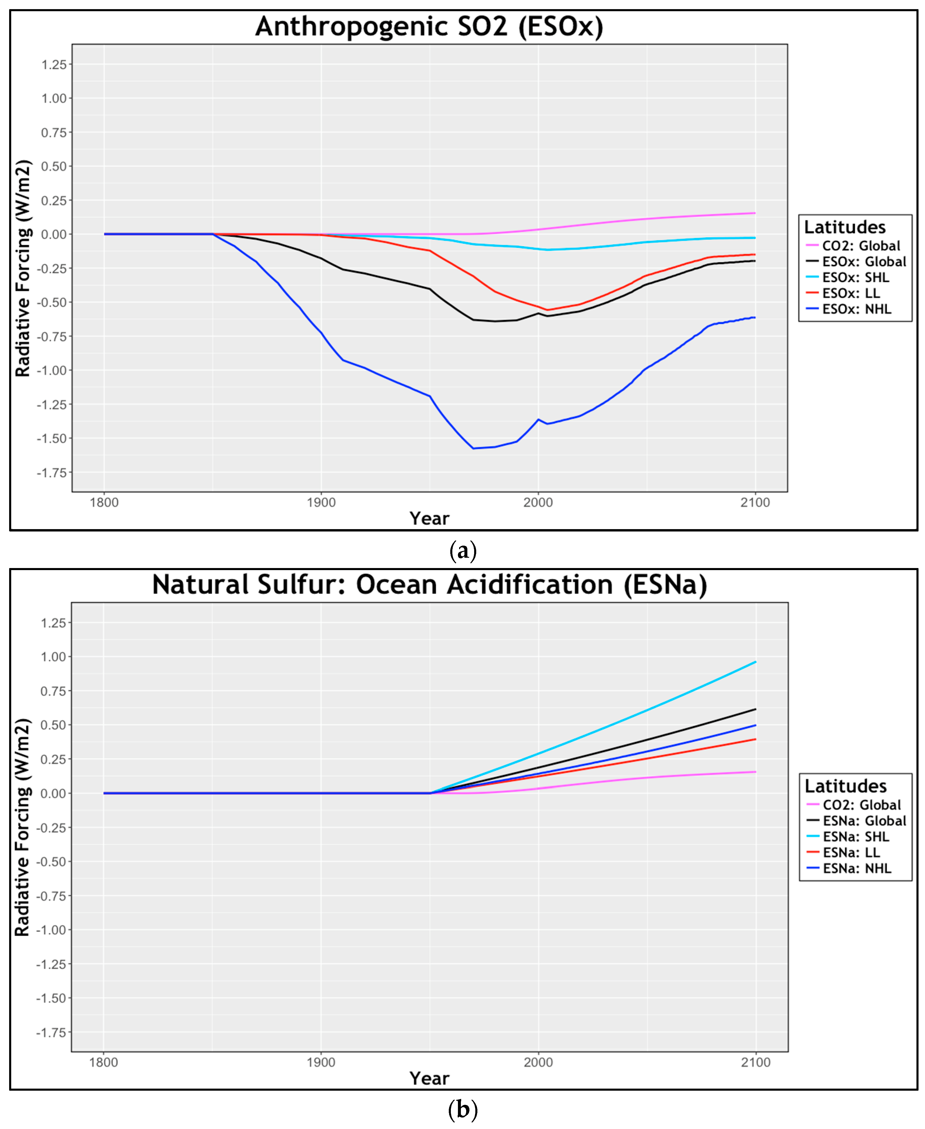
2.1.1. Radiative Forcing: Anthropogenic and ESNa

Equation (2) requires RF values for both natural and anthropogenic sulfur emissions on a global and regional scale. While a planetary anthropogenic sulfur emissions (ESOx) forcing term is supplied by Hector (−0.6 Wm−2), the forcing value needed to be additionally divided in order to determine local variations. A useful table displayed in Smith et al. (2011) [11] tabulated SO2 emissions by country. This enabled a geographical restructuring of pollutants into latitudinal ranges designated for our work—SHL (90–30° S), LL (30–30° N), NHL (30–90° N). To continue a strict methodology of assigning sulfur dioxide emissions, records attributed to “International Shipping” were excluded from local divisions, as they did not have a clear point of origin and produced a negligible flux on a regional scale. However, the vessel’s contributions were reintegrated upon calculation of a global average. A breakdown of values and locations can be viewed in Appendix A. After calculating man-made emissions derived within each hemispheric band, percentage totals were easily evaluated, yielding 5%, 22%, and 64% of the global total for the SHL, LL, and NHL, respectively. These allotments were applied to the planetary average forcing provided by Hector (−0.6 Wm−2), producing values of −0.11, −0.54, and −1.57 Wm−2.
The approach employed for computing RF ESN data could be streamlined due to an image in S13. The image presents change in radiative forcing (Wm−2) from 1865–1874 to 2090–2099 under varying pH-sensitivity scenarios—reference, low, medium, and high situations—ranging from 8.3 to 7.6 pH units. We extracted data from this image and calculated the difference between the high and reference scenarios for the end of century [6]. We utilized this quantity since the intention of our publication is to isolate and observe the effect climate change may have on marine biota and subsequent feedbacks. The global forcing values computed from the image in S13 were then averaged throughout each regional band and across the entire planet: 0.96, 0.40, 0.50, and 0.62 Wm−2, respectively. A list of both ESNa and ESOx forcing values can be found in Table 1.

2.1.2. Anthropogenic Sulfur Emissions

To create a complete anthropogenic sulfur emissions dataset, we expanded the ESOx table described in the previous subsection. For the purpose of calculating an RF term, we focused on pollution from the year 2000. However, Smith et al. only included historical data for the start of each decade—1910, 1920, etc.—between 1850 and 2000 [11]. In order to compute corresponding values for intermediate years, a simple linear regression formula was applied. The periods succeeding the millennium required a companion source of information. The necessary data were found in van Vuuren et al. (2011) describing various representative concentration pathway (RCP) scenarios of human pollutants throughout the 21st century [12]. Since findings from the high pH-sensitivity scenario were used to calculate a radiative forcing value for ESNa, we elected to apply projections under an RCP8.5 future to preserve consistency [6]. Under this pathway, a global average value was provided for each year following 2000. The global average was subsequently divided into the three regional bands using the percentages established for RF computations in Section 2.1.1. (5%, 22%, and 64%). An example calculation can be found in Appendix B.

2.1.3. Natural Sulfur Emissions

At present, there is a shortage of dimethyl sulfide emissions information for both the contemporary era and throughout the coming century. Taking this into consideration, in order to create our ESNa dataset, we again relied on a linear regression formula. First, data for the slope was provided by S13. One of their figures displays the meridional “Change in DMS Flux” from 1865–1874 to 2090–2099 [6]. Next, it was necessary to find emissions by latitude for a single year within the prescribed timeline to act as our reference point. The required statistics have been provided in Simó and Dachs, 2002 [13]. By combining these values, we were able to derive ESNa for each latitude in 1865—the preliminary year chosen by S13—and 2100. As a verification of these methods, natural sulfur emissions in 1865 and 2100 were integrated, giving 29 and 22 TgS year−1, respectively, successfully matching data reported in S13 [6].
A final alteration applied to the data-stream was to impose a “bend” in the estimated slope. This was done to properly reflect the changes of a warming climate as experienced throughout the ocean. Since general consequences of global warming were not readily measurable until the mid-20th century, change in DMS emissions was maintained at 0 until 1950. The inflection point was selected to represent the observed decline of seawater density found by all major Earth system models (ESM), marking the beginning of the measurable impact of climate change on the planet [14]. Following the middle of the century, we imposed a constant slope yielding ESNa values until the year 2100. A compiled spreadsheet of the data and slopes in addition to an example calculation can be found in Appendix B. With all of the required information for the linear regression formula, the remaining values of the ESNa dataset were calculated.

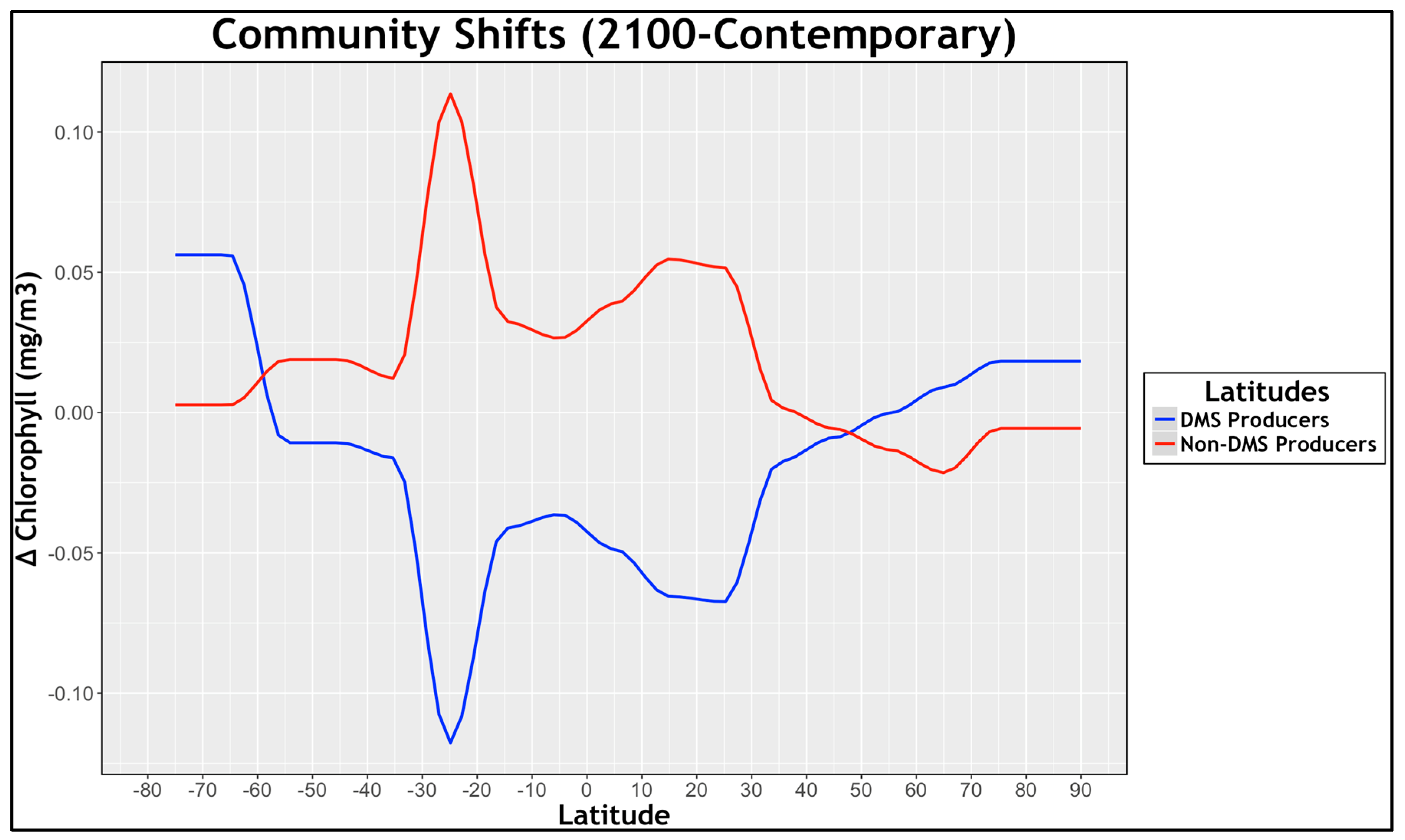
2.2. Community Shifts (ESNc)

Alteration in abundance and habitat of phytoplankton is the second effect explored in our report. For simplicity, in preceding sections, we have defined phytoplankton as a single functional group. However, the remainder of our analysis tested changes which have varying outcomes for the respective classes and required further enumeration. In this context, phytoplankton were organized according to their distinct concentration of the organic sulfur precursor—DMSP. The following portion of our work aims to isolate the major biological forms and to examine the ways in which they are likely to respond to impending changes in climate. The phytoplankton were cataloged as non-DMS producers (cyanobacteria and diatoms) and DMS producers (Phaeocystis, coccolithophorids, along with a dinoflagellate et al. group). By contrast with ocean acidification, this analysis was not accomplished by developing an equation, but rather via an exhaustive synthesis of established data from the beginning and end of century. Example calculations for each functional group before normalization in addition to primary sources of information used can be found in Appendix C. We evaluated variations attributed to nutrient stress, rising sea surface temperature (SST), and increasing exposure to solar irradiance. In keeping with the tone of the “Experiments” section, phytoplankton have been ordered in relation to the data collection methodology, rather than DMS production rates.

2.2.1. Cyanobacteria and Coccolithophorids

The primary source for contemporary phytoplankton distributions is Gregg et al., 2003 [15]. In their work, ESM simulations of chlorophyll abundance attributed to cyanobacteria and coccolithophorids are computed for February and June. These results were averaged to derive an annual value for each latitudinal band. Approximations for coccolithophorids were then correlated with the chance of finding Emiliania huxleyi (EHUX) throughout the global hydrosphere at present and EOC [16]. Using an elementary relation, we calculated a future-to-modern ratio for the probability of EHUX presence and multiplied the result with the current chlorophyll concentrations to tabulate end of century values.
To analyze community shifts for cyanobacteria, data derived from F13 were used [7]. Two picocyanobacterial genera—Synechococcus and Prochlorococcus—demonstrate the growth of cyanobacteria, since they outcompete and supersede their DMS producing counterparts. Flombaum’s group measured the progression of cell abundance, allowing us to establish a percentage change. A minor adjustment was made, since changes reported by F13 were derived from an RCP4.5 scenario. Under these parameters, the ocean would simply warm on average by 1.4 °C relative to 5.5 °C from an RCP8.5 future [12,17]. Operating with outputs from Flombaum and the 4.5 pathway temperature increase, we used a slope to calculate cell count growth under the more severe 8.5 scenario while assuming no differential adaptation to the higher temperatures. Ultimately, these changes were applied to modern values, deriving future concentrations at each latitude.

2.2.2. Phaeocystis

Gathering statistics pertaining to Phaeocystis proved to be the most formidable obstacle for this section of our study. Unlike other species, a great deal of effort was spent trying to find any habitat or concentration data for the foam-producing algae. Unfortunately, we were unsuccessful in obtaining any clear figures, measurements, or other information, and ultimately used an image included in Vogt et al. (2012) reporting cell concentrations from limited depth-resolved stations [18]. As will be shown in subsequent sections, remote sample locations generated extreme sensitivity for the strong DMS emitter. A trivial adjustment to the extrapolated data could significantly influence the overall flux of natural sulfur. Similar to the coccolithophorids calculation, these values were multiplied with a future-to-modern ratio of DMS concentrations associated with the phytoplankton in question, deriving EOC estimations [18,19,20].

2.2.3. Diatoms and Dinoflagellates et al.

Statistics of diatom and small phytoplankton abundance were taken from Marinov et al., 2013 (M13) [21]. Their publication provided an itemized listing of biomass values for diatoms in conjunction with habitat distribution at the beginning and end of century. Information involving small phytoplankton led to the construction of a “catch-all” category for any overflow marine biota which contribute to ESN. As a concession to the finite number of simulations possible, we argue that this group is predominantly populated by dinoflagellates and that their DMS flux would reflect this. Concentrations were collected from diagrams in M13 illustrating small phytoplankton biomass at present and by the year 2100. Quantities associated with the remaining microalgal types—cyanobacteria, Phaeocystis, and EHUX—were then removed from the data, isolating the intended class.

2.2.4. Normalization

As a verification of the data compiled for each functional group, our findings were normalized relative to a table provided in M13. Included in this chart were concentrations for diatoms, small phytoplankton, and total sea surface biota. However, since values for diatoms were taken directly from Marinov’s index, it was not subject to refinement. An added complication to the process arose as each group was subdivided into imprecise biome regions such as Equatorial or Subtropical Northern Hemisphere. While aided by an image representing the author’s intent for these habitats, we had to use expert judgment when assigning various locations into distinct latitudinal zones. This was not possible in two meridional portions to the north (40–50° N and 60–70° N). Within these settings, no clear biome dominated the bands and, instead, a linearization from the proximal ecosystem categories was imposed [21].
Once arranged into appropriate domains, estimates from the methods explored in preceding subsections were refined relative to measurements found in M13 [21]. We first calculated the ratio of small to total plankton within each biome. These percentages provided a scale, which was then used to adjust our phytoplankton values to produce a total concentration equivalent to that reported by Marinov. As a supplement to the process, since findings by Vogt et al. had a deficiency of Phaeocystis data at SHL, we scaled results between 60–80° S to represent the established presence of the predominant DMS producer [19]. A complete breakdown of each functional group from present day and end of century after normalization can be found in Table 2.

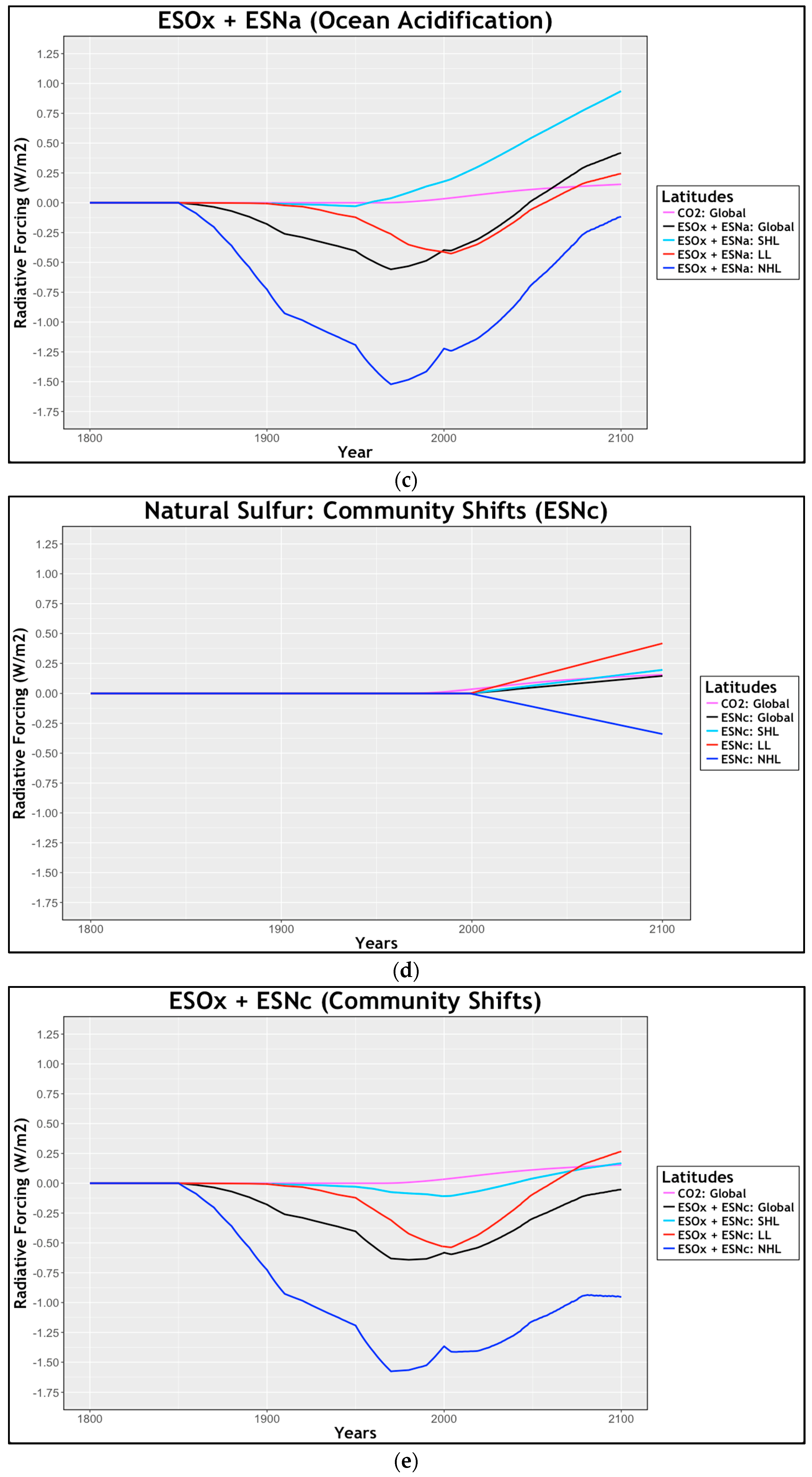
2.2.5. Radiative Forcing: Community Shifts

The final step for assessing outcomes from planktonic community shifts was to relate marine biotic concentrations to their corresponding impact on the global radiative budget. Beginning with a few simple conversions, values from Elliott (2009) [22] provided average N:S ratios, which were used to calculate sulfur concentrations (Cj) for each functional group. Additionally, this report included percentage yields (Y) for dimethyl sulfide from its precursor—DMSP. These quantities were then substituted into the following expression:
S o u r c e D M S = g · Z · ( C j K 3 ) · Y
Equation (3) was adopted and adapted from a grazing rate equation found in Sarmiento et al. (1993) [23]. The calculation determines the frequency with which DMSP is released via predation and the consequent formation of DMS. In this context, (g) is a shorthand for maximum growth rate and (K3) is a stand-in for half saturation ingestion. These constants were assigned to be 1 day−1 and 1 mmolN m−3 respectively. Finally, (Z) denotes zooplankton concentrations which were listed in M13 [21].
The next step in the process was to quantify a DMS time constant:
T i m e   C o n s t a n t D M S = ( k B · ( 0.1 · ( N P ) 0.5 ) ) 1
In the simple Equation (4), ( k B ) is the bacterial kinetic coefficient, assumed to be 30 (day mmolN m−3)−1. The second term represents concentration of bacteria, which is itself a function of phytoplanktonic nitrogen (Np) [22]. Net dimethyl sulfide flux was then found by multiplying frequency of production (Equation (3)), the DMS time constant (Equation (4)), and the appropriate piston velocity [24]. In order to match accepted dimethyl sulfide emissions, results had to be scaled by a factor of 5 [25]. Returning to S13, latitudinal correlations were evaluated using the data reported in the figures “Change in DMS Flux” and “Radiative Forcing”. These associations were used to convert our calculated emission rates to RF values, both regionally and globally. Finally, the calculated changes in radiative forcing were added, offline, to the original anthropogenic emissions to estimate the total sulfur cycle with respect to phytoplanktonic community shifts.

2.3. CO2 mBGC Feedback

One of the goals of the present work is to demonstrate the influence marine ESN have on the global radiative budget, both historically and in future decades. In order to give context to our findings, results were compared to the forcing agent most familiar throughout the scientific community—anthropogenic carbon dioxide. This requires an examination of the feedback effect CO2 and marine biota have on one another. Unfortunately, Hector itself does not include a representation of the biological pump at this time and could not be used for our intended purposes. Instead, one of the authors (CH) provided a simplified model of the carbon ocean component from Hector in an Excel format. This allowed us to easily add in equations and track the flow of carbon throughout the ocean. The document served as a skeletal structure, which we developed to include an atmosphere in addition to a solubility and biological pump. Initial values for the various reservoirs were taken from Watson and Liss (1998), and the solubility pump is based on the formula outlined in Sarmiento and Gruber (2006) [26,27]. The inclusion of the solubility pump required representation of the carbon cycle chemistry as a function of time in both surface ocean reservoirs. The model was ultimately parameterized to ensure this flux paralleled historical and projected concentrations to represent the changes to climate, including ocean acidification, accurately. Forcings attributed to CO2 emissions were then calculated using the expression found in Hector:
R F CO 2 = 5.35 × l n C a C 0
Equation (5) assigns 5.35 Wm−2 as a scaling factor in addition to requiring both the initial and current atmospheric concentrations (Ca, C0). The starting value was set at 278 ppm [9,28].

Biological Pump

Within our Excel-Hector, the biological pump is represented using two formulas, both of which are a function of annual mean surface nitrate concentrations (N) [27]:
B i o l o g i c a l   P u m p S u r f a c e = R · N · ( 1 Rm )
B i o l o g i c a l   P u m p I n t , D e e p = R · N · ( Rm )
In Equations (6) and (7), (R) is the standard Redfield ratio used to convert the controlling element into carbon values and (Rm) signifies the remineralization percentage, which determines the amount of nitrate that will remain at the respective depths [29]. Equation (6) is subtracted from reservoirs calculated in the mixed layer at both high and low latitudes, while Equation (7) is added to the intermediate and deep equivalent, ensuring both conservation of nitrogen atoms and the preservation of nitrate abundance. The utilization of both expressions allows for control of the biological sequestration rate, which we vary throughout the present century.
To ensure accuracy of the model, inputs were set to calculate: (1) a biological pump strength of −120 ppm for the present day; and (2) an additional 30 ppm in the atmosphere by EOC relative to a climate change free reference run [30,31]. It should be noted that the decrease in biopump efficiency attributed to global warming is greater than that reported in analogous models [32]. This exaggerated difference was chosen to demonstrate the potential significance of DMS relative to an extreme baseline. Nitrate values were held constant from initialization of the model through 1950, and then follow a linear decay to endpoints prescribed during parameterization. The midcentury date was chosen to parallel our DMS examination (refer to Section 2.1.3) [14]. A complete listing of data used can be found in Appendix D.

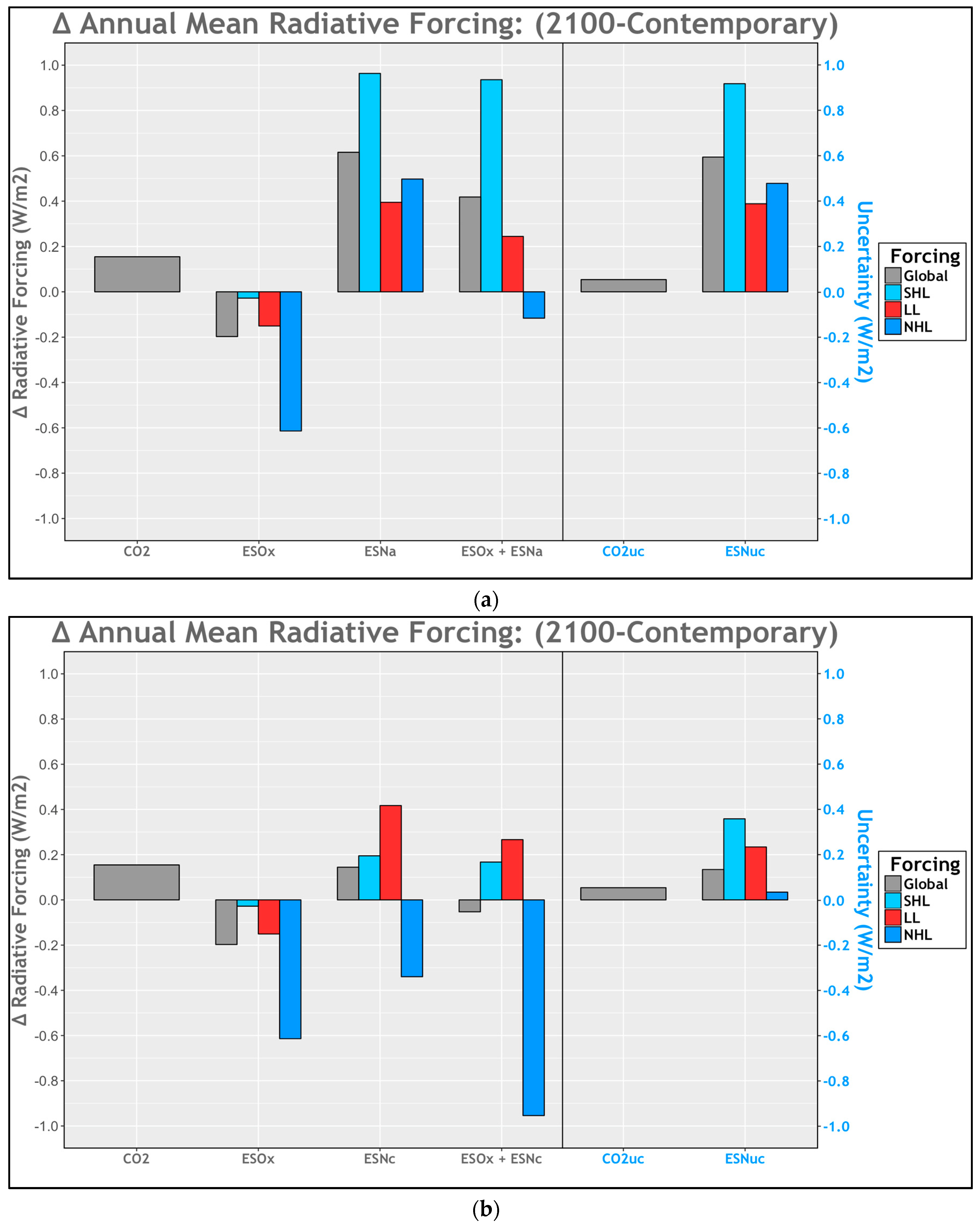
2.4. Sensitivity Tests (ESNuc, CO2uc)

Limited available data proved to be a continual challenge throughout this investigation. As such, findings from the present work were subjected to a series of sensitivity tests to calculate ranges of uncertainty. Each assessment was conducted separately: an adjustment was made to our results, the corresponding output was calculated, and the data were reverted to the original state before the analysis continued. All results from these tests are illustrated and explored at greater depth in Section 3.4.

2.4.1. Uncertainty: Ocean Acidification

First, we reevaluated claims made in S13. Considering our experiment utilized their high acidification scenario, an exercise was designed to determine results for a low-end outcome [6]. The test focused on the fact that, while diminishing pH levels will affect all marine biota, calcium shells surrounding coccolithophores result in a greater susceptibility for their community. Therefore, we computed the ratio of EHUX to total phytoplankton concentrations and multiplied the result with the change in radiative forcings by EOC. This effectively isolated the impact of coccolithophores, which was then subtracted from our ∆RF to determine the extent of uncertainty.

2.4.2. Uncertainty: Community Shifts

To verify our community shift findings, we designed a test for each of the three meridional zones. The low latitude assessment focused on F13’s picocyanobacterial data derived from an RCP4.5 scenario [7]. As previously stated, in order to keep EOC outcomes consistent throughout this investigation, we had to scale Flombaum’s output to match an RCP8.5 temperature increase. Therefore, we decided it was appropriate to calculate the difference between our results and the anticipated changes reported by F13.
For both high-latitude regions, the greatest source of uncertainty came from contemporary Phaeocystis data found in Vogt et al. [18]. In this particular report, it is explained that measurements were taken from remote stations, resulting in a thorough analysis of the Arctic Ocean and an underrepresentation of its southern counterpart. Unfortunately, alterations could not be made directly to Vogt’s findings due to subsequent modifications of the data. Instead, the normalized small phytoplankton biomass was: (1) cut in half between 50–60° N; and (2) scaled an additional 10 times in the Southern Hemisphere ice biome to match accepted annual DMS emissions [21,25]. Although the latter adjustment may appear to be excessive, we believe it further validates the necessity for additional DMS investigations. Throughout the present work, we were limited to a single report regarding Phaeocystis, resulting in striking modifications, such as those used to produce acceptable statistics [18].
An additional test was conducted in the SHL, focusing on the projected change in Phaeocystis abundance. Estimated data from model output used for our analysis reflect approximately a 50% decrease in Phaeocystis by EOC [20]. However, in the current literature, there are also publications which suggest a poleward migration of the genus [8]. Considering these potentially contrasting scenarios, we changed the decline in concentration to 10%. Finally, outputs from all three sensitivity tests in addition to the reference run were compared, and both the high and low values were determined, producing our uncertainty ranges.

2.4.3. Uncertainty: CO2

Currently, a considerable amount of scientific and Earth system modeling attention is given to reducing the uncertainty associated with anthropogenic CO2. This level of refinement is in contrast with the present work, which demonstrates the many improvements still necessary for contemporary or projected ESN data. To quantify this discrepancy, we reviewed the current literature to determine an acceptable range of warming attributed to CO2 and a waning biological pump. According to the fifth Coupled Model Intercomparison Project, by the end of century, atmospheric concentrations are expected to increase due to feedback by 50–100 ppm, with <20% attributed to the global aquatic ecosystem [31,32]. This suggests an increase of 10–20 ppm from the carbon dioxide mBGC interaction. Excel-Hector was reparametrized with both a 10 and 20 ppm change in biopump strength, relative to the reference EOC value, and rerun to calculate the respective ∆RF for the accepted range.

3. Results

3.1. Anthropogenic Sulfur Emissions (ESOx)

In its present configuration, Hector uses Equation (1) to quantify anthropogenic sulfur pollutants while holding natural emissions constant (Figure 1a). Throughout the modern century, both local and global ESOx share characteristic trends to varying degrees. Between 1850 and 1900, the forcings begin to decrease, resulting in negative RF values, reaching a minimum between 1970 and 2000. Following these inflection points, under an RCP8.5 scenario, all outcomes begin and continue to rise until EOC. This increase can be attributed to a growing effort from industrialized nations to reduce their contribution of sulfur dioxide to climate. We observe the greatest decline in RF at northern high latitudes, since they host a majority of polluting nations. This region reaches a minimum value of −1.58 Wm−2 in 1970. The negative radiative forcing reduces the global average, causing the planetary mean to have the second-lowest RF value in the plot. Worldwide irradiance reaches −0.6 Wm−2 in the year 2000, suggesting Equation (1) is performing as anticipated. The low-latitude outcome follows the same characteristic pattern but on a mitigated scale, reflecting the smaller number of developed countries. Finally, the Southern Ocean experiences a minimal decline—attributable mainly to South Africa and Australia—before stabilizing near 0 Wm−2.

3.2. Natural Sulfur Emissions: Ocean Acidification (Esna)

Figure 1b isolates our addition to the standard indirect sulfate aerosol equation. Adopting the methods and data reported in S13, linear slopes are imposed. Starting in the 1950s, each function begins to show the impact of ocean acidification. Due to the high phytoplanktonic concentration in the Southern Ocean, the largest rise in forcing is observed at SHL, reaching a value of 0.96 Wm−2 by EOC. Analogous to ESOx, this large local growth was the dominant factor governing the global average. The planetary mean has the second-highest value among the RF at 0.62 Wm−2, representing a possible impact 4 times that of marine carbon cycle feedback. Ultimately, Equation (2)—characterizing both man-made and natural sulfur emissions—was used in Hector to compute values shown in Figure 1c. The effect of a dynamic ESN component is evident, since the increase in radiative forcing substantially shifts end of century values. Introducing DMS emissions effectively reversed the sign in all regional and global divisions, barring northern high latitude. These combined components result in a planetary average of 0.42 Wm−2.

3.3. Natural Sulfur Emissions: Community Shifts (ESNc)

Distinct from the changes explored in the previous subsection, shifts in community structure result in both intensification and reduction to the RF. As seen in Figure 1d, northern high and low latitudes exhibit opposite trends in the 21st century. By the year 2100, LL values approach 0.42 Wm−2, effectively balancing the decline to −0.34 Wm−2 at NHL on the global average. An unexpected outcome of biogeographic evolution was observed in the south. Since ecosystems in the SHL experience environmental changes similar to the northern counterpart, both were anticipated to adjust in a comparable manner. However, the increase in radiative forcing at SHL suggests a loss of DMS-producing biota. A working hypothesis for the divergent behavior is again associated with limited Phaeocystis records. The few stations collecting Phaeocystis data near Antarctica develop a disproportionate representation between 60° S and 80° S. Therefore, similar percentage losses experienced near both poles lead to a greater decline in the southern population and, by extension, DMS emission rates.
A final community shift graph was produced representing the collective anthropogenic and natural sulfur forcings (Figure 1e). The new trends show phytoplankton relocation countering man-made emissions in both low and southern regions, leading to a positive radiative forcing by 2100. However, in NHL, changes in the marine biota have an amplifying effect on the sulfur pollutant. These contrasting outcomes nearly balance one another, reducing any changes from a global perspective.

Change in Total Chlorophyll Concentration: (RCP8.5–Contemporary)

An alternate representation of community shifts shows the change in chlorophyll concentration between end-of-century and modern-day simulations (Figure 2). Established data of phytoplanktonic classes were synthesized and organized into two groups: DMS producers (Phaeocystis, EHUX, dinoflagellates et al.) and non-DMS producers (cyanobacteria, diatoms). Figure 2 illustrates the results reported in Table 2, since the latitudinal trends follow qualitative projections in the current body of literature.
Next to Antarctica, there is an increase in DMS producers. Although this seems counterintuitive relative to the results reported in the preceding subsection, our projected growth for the dinoflagellate group outweighs any loss of Phaeocystis. Ultimately, the shift to a somewhat weaker producer will reduce DMS emissions but increase the total chlorophyll concentration. Between 60° S and 30° S, there is a migration poleward of DMS-producing plankton and consequent replacement by diatoms. Low latitudes show a growing dominance of cyanobacteria under reduced nitrate abundance and rising SST. These small algae supersede the strong dimethyl sulfide-emitting plankton. An increase in non-DMS producers reaches a peak at 25°, representing maximal expansion of cyanobacteria and minimal reduction to the diatom population. Although the equatorial band is dominated by Synechococcus and Prochlorococcus, there is not an equivalent maximum at the Intertropical Convergence Zone (ITCZ), as reported in F13 [7]. This is a consequence of the normalization process explained in Section 2.2.4. Finally, in NHL, there is a small decline in diatom abundance with a trough at 65° N and a concurrent growth of the dinoflagellate et al. group, which stabilizes moving toward the pole.

3.4. Histograms

We conclude the results section with two histograms summarizing all outcomes generated during our analysis. This type of chart was chosen for Figure 3 to allow for direct comparison to radiative forcings plots reported in external publications [33]. Both of the figures begin with changes in RF due to the anthropogenic CO2 mBGC feedback and SO2 pollutants. Next are the changes in forcing attributed to dynamic ESN with respect to ocean acidification and community shifts—Figure 3a,b, respectively. Finally, the natural and man-made combined influence on the global radiative budget are shown. Positioned directly to the right of the dividing line there are visual representations of the sensitivity tests discussed in Section 2.4. In Figure 3a, uncertainty for global natural sulfur emissions with respect to acidification is more than six times that of CO2 mBGC feedback. This demonstrates the need for further quantitatively driven analyses, and for refinement of the current knowledge base. Results for uncertainty in ESN while analyzing community shifts (Figure 3b) are smaller, and the global average is comparable to that of carbon dioxide. In both figures, the greatest source of uncertainty is in the prime habitat of phytoplankton, the Southern Ocean. It should be noted that values used for these plots are from EOC and lie beyond the RF troughs reported from anthropogenic emission at the start of the century.

4. Discussion

The present work constitutes an in-depth evaluation of ESN from marine ecosystems between the preindustrial era and 2100 under a “business as usual” emissions scenario. In an attempt to examine changes projected for DMS-producing plankton, separate analyses were conducted for ocean acidification and ecological community shifts to isolate their respective impacts. All of our findings are reported from both a global and regional scale to provide a new perspective on the complicated dynamics of natural sulfur emissions. Several of the local projections of phytoplankton community shifts show different and sometimes opposing variations. Results such as these explicitly address the complex nature of researching natural dimethyl sulfide production as a planetary average. For example, attributed to a warming climate, we observe an expansion of cyanobacteria near the equator, reducing DMS emissions. Yet, in the Arctic Ocean, poleward migration of eukaryotes results in the opposite effect. Although such changes are contradictory, they serve as indications for their respective ecosystems. Even when future trends are internally consistent—as is the case with ocean acidification—large localized outcomes can be overlooked. We quantified a worldwide reduction in phytoplanktonic abundance with an impact nearly three times greater in SHL relative to other latitudinal zones and approximately double the global output.
To the best of the author’s knowledge, the present investigation is the first attempt at a regional scale analysis of multiple natural sulfur emissions effects with respect to climate change. Currently, the dimethyl sulfide indirect effect is not acknowledged as either a feedback or forcing source in the RF chart presented perennially in IPCC reports [33]. The absence from high profile review material forced us to use data reported throughout several sources, restricting techniques used to simple linearization and estimations. Consequently, high uncertainty is associated with most of the conclusions produced from these methods. Yet, even when taking such challenges into consideration, results reported here address the realistic probability that ESN may have an influence up to four times that of the CO2 marine biogeochemical feedback on radiative forcing, with regional complications in addition. Ultimately, results from the present work attempt to quantify the role natural sulfur emissions may play in the planetary radiative forcing budget, demonstrating the need for further examination.

5. Conclusions

Although DMS gained recognition throughout the scientific community via the CLAW hypothesis, it is often still discussed in a qualitative manner. Recently, scientists have begun to take a more comprehensive approach to analyzing the role natural sulfur may play in global climate [6,8,19]. The present work contributes to this effort by: (1) synthesizing findings from numerous articles and experiments which study upcoming changes to sulfur producing plankton; and (2) analyzing global projections on a latitudinal basis by separating the planetary data into three meridional zones—SHL (90–30° S), LL (30–30° N), and NHL (30–90° N).
Our investigation began with a review of the current representation of ESN in a simplified climate model, Hector. We found that Hector results matched analogous simulations with fixed DMS emissions, minimizing any influence natural sulfur may have [10]. Therefore, as a first attempt to calculate the dynamic effect dimethyl sulfide will exert on the radiative budget, a supplementary term was added to the SCM (Equation (2)). Our approach developed the new expression following the format currently used for SO2 forcings (Equation (1)) and the acidification data reported in S13 [6]. Next, we studied the remaining sulfur-related potential consequences of climate change—nutrient depletion, sea surface warming, increased light availability—and their impact on major phytoplanktonic classes of diverging DMS production. Assessments of the functional taxonomic groups were not done within Hector, since the interactions were too intricate to replicate numerically. Instead, the algal types were categorized based on their ability to produce DMS, and concentrations were collected from ESM outputs simulating the beginning and EOC. The values were then converted into forcing terms and added to outcomes from the original anthropogenic equation (Equation (1)).
Beyond traditional results considered in the previous sections, an important outcome presented in this report is the need for more dimethyl sulfide mBGC feedback data. Not only was our addition to Hector the first attempt at including a dynamic ESN component within a simplified climate model, it also uses linearized data based on an external publication [6,9]. Likewise, the limited number of EOC simulations for major sulfur-producing phytoplankton forced the synthesized data to be normalized and scaled to match accepted annual DMS emissions [25]. Such methods are currently necessary to conduct a proper investigation of natural sulfur emissions. However, with continued simulations and measurements, the amount of required modification can likely be reduced. To this end, all statistics, formulas, and resources used in the investigation are included in the text proper or in a series of appendices. We are optimistic that the information collected can be further applied to expand and verify the methodologies and results presented in this work. With the future of biogeochemical feedbacks so uncertain, the scientific community must continuously advance our understanding of changes the planet will experience in coming decades. Such a complex problem warrants a comprehensive analysis of each compound, which could act as a forcing agent. This task requires us to move beyond familiar aspects of the radiative budget and explore all facets of the climate system.

Author Contributions

Z.M. and S.E. conceived and designed the experiment; Z.M. performed the experiments; Z.M. and S.E. analyzed the data; C.H., F.H., and S.W. contributed materials and analysis tools; Z.M. wrote the paper.

Acknowledgments

Authors of this publication thank JGCRI for their time and expertise as we implemented the simple climate model. This research was supported through the Reducing Uncertainties in Biogeochemical Interactions through Synthesis and Computation (RUBISCO) and High Latitude (HiLAT) Scientific Focus Areas, which are sponsored by the Regional & Global Climate Modeling (RGCM) Program in the Climate and Environmental Sciences Division (CESD) of the Biological and Environmental Research (BER) Program in the U.S. Department of Energy Office of Science.

Conflicts of Interest

The authors declare no conflict of interest.

Appendix A

Table A1. Anthropogenic sulfur emissions and radiative forcing vales for the year 2000, reordered into regional sections [11].
AreaESOx (Gg)
USA and Canada17,054
Western Europe7998
Central Europe5704
Russia6352
Ukraine1548
Other Former Soviet Union2516
China21,393
Japan885
Middle East5218
Northern High Latitude Total:68,668
Mexico2991
Central America867
South America4719
Other South and East Asia6330
India5363
Africa3322
Low Latitude Total:23,592
South Africa2392
Australia and New Zealand2438
Southern High Latitude Total:4830
International Shipping:9779
Global Total:106,869

Appendix B

Equations (A1) and (A2). An example calculation of ESOx at southern high latitudes. Historical data reports anthropogenic emissions at SHL in 1980 as 3552 Gg SO2 and 3931 Gg SO2 in 1990 [11]. In 2050, an RCP8.5 scenario projects a global sulfur dioxide emissions rate to be 50.9 Mt(S) year−1 [12]. The southern high latitude region currently contributes 4.5% of global sulfur pollutants—as explained in Section 2.1.1. Equation (A1) demonstrates the use of the linear regression formula to calculate annual values. Equation (A2) shows how the total global emissions are apportioned into the SHL region.
ESOx 1985 = ( 3931 3552 10 ) · 5 + 3552 = 3741.5   Gg   SO 2
ESOx2050 = 50.9 · 0.045 = 2.3 Mt(S) year−1
Equations (A3)–(A6). An example calculation of ESN with respect to ocean acidification between 50 and 60° S. The change in DMS emissions from 1865 to 2099 is −0.0024 TgS year−1 and ESN in the year 2000 was 1.11 TgS [6,13]. In Equations (A3) and (A4), the linear regression formula is used to find emission values in the preliminary year (1865) and 2099. Equation (A5) illustrates that after imposing the “bend” technique—explained in Section 2.1.3—the ESN value between 1865 and 1950 is held constant. Finally, in Equation (A6), the new slope from 1950 to 2099 is calculated.
ESNa1865 = 1.11 + 0.0024 · (2000 − 1865) = 1.43 TgS
ESNa2099 = −0.0024 · (2099 − 1865) + 1.43 = 0.87 TgS
ESNa1950 = ESNa1865 = 1.43 TgS
ESNa 1950 2099 = ( 0.87 1.43 2099 1950 ) = 0.0038   TgS   year 1
Table A2. Natural sulfur emissions (TgS) and slopes (TgS yr−1) by latitude. Included in order: natural sulfur emissions in the year 2000, slopes used for the entire period, natural sulfur emissions in the year 1865, natural sulfur emissions in the year 2099, and slopes used between 1950 and 2099 [6,13].
LatitudeESN2000ESN2099–1865ESN1865ESN2099ESN2099–1950
90–80° S:0.0000.00000.0000.0000.0000
80–70° S:0.0170.0003−0.0200.0460.0005
70–60° S:0.373−0.00010.3860.363−0.0002
60–50° S:1.113−0.00241.4300.867−0.0038
50–40° S:2.033−0.00332.4451.707−0.0051
40–30° S:2.127−0.00522.7841.606−0.0082
30–20° S:2.237−0.00472.8221.773−0.0073
20–10° S:2.593−0.00353.0272.249−0.0054
10–0° S:2.817−0.00413.3282.412−0.0063
0–10° N:3.387−0.00353.8213.042−0.0054
10–20° N:2.860−0.00403.3592.464−0.0062
20–30° N:1.563−0.00291.9251.276−0.0045
30–40° N:1.297−0.00301.6780.994−0.0047
40–50° N:0.833−0.00371.2950.467−0.0057
50–60° N:0.500−0.00200.7570.296−0.0032
60–70° N:0.147−0.00060.2270.083−0.0010
70–80° N:0.2000.00010.1860.2110.0002
80–90° N:0.0030.0002−0.0220.0230.0003
Global Average1.339−0.00241.6351.104−0.0037

Appendix C

Equation (A7). An example calculation of coccolithophorids between 30 and 40° S. Contemporary concentrations for coccolithophorids is 0.009 mg Chl. m−3 and a 31% chance of EHUX being present [15,16]. Future probability of EHUX presence is 27.3% [16]. Equation (A7) demonstrates the calculation of future coccolithophorids abundance.
Coccolithophorids 2100 = ( 0.009 0.310 ) · 0.273 = 0.008   mg   Chl .   m 3
Equations (A8)–(A10). An example calculation of the cyanobacteria between 20 and 30° N. Contemporary concentration for total cyanobacteria is 0.108 mg Chl. m−3 and 69,454 cell mL−1 for Prochlorococcus and Synechococcus cell abundance [7,15]. The future estimation for Prochlorococcus and Synechococcus under an RCP4.5 is 93,266 cell mL−1 [7]. Temperature of the global oceans will rise on average by 1.4 and 5.5 °C under RCP4.5 and 8.5 scenarios, respectively [12,17]. Equation (A8) uses the linear regression formula to extrapolate cell abundance under an RCP8.5 projection. Next, Equation (A9) uses the cell concentration for present day and under an RCP8.5 future to calculate the growth. Finally, in Equation (A10), the percentage growth is multiplied by the modern-day total cyanobacteria value to determine EOC data.
Cell   Abundance RCP 8.5 = ( 93,266 69,454 1.4 ) · 5.5 + 69,454 = 163,001   cell   mL 1
Growth = ( 163,001 69,454 ) = 2.35
Cyanobacteria2100 = 0.108 · 2.35 = 0.254 mg Chl. m−3
Equation (A11). An example calculation of Phaeocystis between 40 and 50° S. Contemporary concentration for Phaeocystis is 0.042 mg Chl. m−3 and DMS emission from Phaeocystis is 0.064 nM [18,19]. Future estimations of DMS emission from Phaeocystis is 0.11 nM [20]. Equation (A11) demonstrates the calculation of EOC Phaeocystis abundance.
P h a e o c y s t i s 2100 = ( 0.042 0.064 ) · 0.11 = 0.072   mg   Chl .   m 3
Equations (A12) and (A13). An example calculation of the dinoflagellates et al. group between 0 and 10° N. Contemporary concentration of total small phytoplankton is 0.19 mg Chl. m−3 and the combined abundance of cyanobacteria, Phaeocystis, and coccolithophorids is 0.07 mg Chl. m−3 [15,18,21]. Change in total small phytoplankton by EOC is projected to be −0.012 mg Chl. m−3 and the estimated change of the aggregate concentration of cyanobacteria, Phaeocystis, and coccolithophorids is 0.060 mg Chl. m−3 [7,15,16,18,19,20,21].
Dinoflagellates et al.Contemporary = 0.19 − 0.07 = 0.12 mg Chl. m−3
Dinoflagellates et al.2100 = −0.012 − 0.060 = −0.072 mg Chl. m−3
Table A3. The primary sources of information used for each of the functional groups for present day and end of century.
Functional GroupContemporaryEnd of CenturyReference
CyanobacteriaGregg et al., 2003Gregg et al., 2003
Flombaum et al., 2013
[7,15]
CoccolithophoridsGregg et al., 2003Gregg et al., 2003
Jensen et al., 2017
[15,16]
PhaeocystisVogt et al., 2012Vogt et al., 2012
Wang et al., 2015
Wang et al., (In Review)
[18,19,20]
DiatomsMarinov et al., 2013Marinov et al., 2013[21]
Dinoflagellates et al. Marinov et al., 2013
Gregg et al., 2003
Vogt et al., 2012
Marinov et al., 2013
Gregg et al., 2003
Flombaum et al., 2013
Jensen et al., 2017
Vogt et al., 2012
Wang et al., 2015
Wang et al., (In Review)
[7,15,16,18,19,20,21]

Appendix D

Table A4. Parameterization values prescribed for Excel-Hector in each reservoir: atmosphere, surface low latitude, surface high latitude, intermediate, and deep ocean. Values include in order: initial carbon (PgC), piston velocity (m s−1), remineralization percentages, nitrate concentrations in the year 1745 (mmol m−3), and nitrate concentrations in the year 2100 (mmol m−3). The two percentages included for the intermediate remineralization represent: SLL to intermediate ocean and (SHL to intermediate ocean).
ReservoirInitial (PgC)PV (m s−1)RemineralizationNitrate1745 (mmol m−3)Nitrate2100 (mmol m−3)
Atmosphere750----
Surface Low Latitude Ocean8502.01 × 10−579%52
Surface High Latitude Ocean2003.12 × 10−560%1515
Intermediate Ocean9600-21% (40%)--
Deep Ocean26,400----

References

  1. Kloster, S. DMS cycle in the ocean-atmosphere system and its response to anthropogenic perturbations. Rep. Earth Syst. Sci. 2006, 103, 1–103. [Google Scholar]
  2. Stefels, J.; Steinke, M.; Turner, S.; Malin, G.; Belviso, S. Environmental constraints on the production and removal of the climatically active gas dimethylsulphide (DMS) and implications for ecosystem modeling. Biogeochemistry 2007, 83, 245–275. [Google Scholar] [CrossRef]
  3. Schwinger, J.; Tjiputra, J.; Goris, N.; Six, K.; Kirkevåg, A.; Seland, Ø.; Heinze, C.; Ilyina, T. Amplification of global warming through pH-dependence of DMS-production simulated with a fully coupled Earth system model. Biogeosci. Discuss. 2017, 20, 1–26. [Google Scholar] [CrossRef]
  4. Charlson, R.J.; Lovelock, J.E.; Andreae, M.O.; Warren, S.G. Oceanic phytoplankton, atmospheric sulphur, albedo and climate. Nature 1987, 326, 655–661. [Google Scholar] [CrossRef]
  5. Menzo, Z.M. Web strategy to convey marine biogeochemical feedback concepts to the policy community: Aerosol and sea ice. Atmosphere 2018, 9, 22. [Google Scholar] [CrossRef]
  6. Six, K.D.; Kloster, S.; Ilyina, T.; Archer, S.D.; Zhang, K.; Maier-Reimer, E. Global warming amplified by reduced sulphur fluxes as a result of ocean acidification. Nat. Clim. Chang. 2013, 3, 975–978. [Google Scholar] [CrossRef]
  7. Flombaum, P.; Gallegos, J.L.; Gordillo, R.; Rincón, J.; Zabala, L.L.; Jiao, N.; Karl, D.; Li, W.K.W.; Lomas, M.; Veneziano, D.; et al. Present and future global distributions of the marine Cyanobacteria Prochlorococcus and Synechococcus. Proc. Natl. Acad. Sci. USA 2013, 110, 9824–9829. [Google Scholar] [CrossRef] [PubMed]
  8. Cameron-Smith, P.; Elliott, S.; Maltrud, M.; Erickson, D.; Wingenter, O. Changes in dimethyl sulfide oceanic distribution due to climate change. Geophys. Res. Lett. 2011, 38, 1–5. [Google Scholar] [CrossRef]
  9. Hartin, C.A.; Patel, P.; Schwarber, A.; Link, R.P.; Bond-Lamberty, B.P. A simple object-oriented and open-source model for scientific and policy analyses of the global climate system—Hector v1.0. Geosci. Model Dev. 2015, 8, 939–955. [Google Scholar] [CrossRef]
  10. Joos, F.; Prentice, C.; Sitch, S.; Meyer, R.; Hooss, G.; Plattner, G.K.; Gerber, S.; Hasselmann, K. Global warming feedbacks on terrestrial carbon uptake under the intergovernmental Panel on Climate Change (IPCC) emission scenarios. Glob. Biogeochem. Cycles 2001, 15, 891–907. [Google Scholar] [CrossRef]
  11. Smith, S.J.; Van Aardenne, J.; Klimont, Z.; Andres, R.J.; Volke, A.; Delgado Arias, S. Anthropogenic sulfur dioxide emissions: 1850–2005. Atmos. Chem. Phys. 2011, 11, 1101–1116. [Google Scholar] [CrossRef] [Green Version]
  12. Van Vuuren, D.P.; Edmonds, J.; Kainuma, M.; Riahi, K.; Thomson, A.; Hibbard, K.; Hurtt, G.C.; Kram, T.; Krey, V.; Nakicenovic, N.; et al. The representative concentration pathways: An overview. Clim. Chang. 2011, 109, 5–31. [Google Scholar] [CrossRef]
  13. Simó, R.; Dachs, J. Global ocean emission of dimethylsulfide predicted from biogeophysical data. Glob. Biogeochem. Cycles 2002, 16. [Google Scholar] [CrossRef]
  14. Fu, W.; Randerson, J.T.; Keith Moore, J. Climate change impacts on net primary production (NPP) and export production (EP) regulated by increasing stratification and phytoplankton community structure in the CMIP5 models. Biogeosciences 2016, 13, 5151–5170. [Google Scholar] [CrossRef]
  15. Gregg, W.W.; Ginoux, P.; Schopf, P.S.; Casey, N.W. Phytoplankton and iron: Validation of a global three-dimensional ocean biogeochemical model. Deep-Sea Res. Part II Top. Stud. Oceanogr. 2003, 50, 3143–3169. [Google Scholar] [CrossRef]
  16. Jensen, L.Ø.; Mousing, E.A.; Richardson, K. Using species distribution modelling to predict future distributions of phytoplankton: Case study using species important for the biological pump. Mar. Ecol. 2017, 38. [Google Scholar] [CrossRef]
  17. NOAA Climate Model: Temperature Change (RCP 8.5)—2006–2100. Available online: https://sos.noaa.gov/datasets/climate-model-temperature-change-rcp-85-2006-2100 (accessed on 15 August 2017).
  18. Vogt, M.; O’Brien, C.; Peloquin, J.; Schoemann, V.; Breton, E.; Estrada, M.; Gibson, J.; Karentz, D.; Van Leeuwe, M.A.; Stefels, J.; et al. Global marine plankton functional type biomass distributions: Phaeocystis spp. Earth Syst. Sci. Data 2012, 4, 107–120. [Google Scholar] [CrossRef]
  19. Wang, S.; Elliott, S.; Maltrud, M.; Cameron-Smith, P. Influence of explicit Phaeocystis parameterizations on the global distribution of marine dimethyl sulfide. J. Geophys. Res. G Biogeosci. 2015, 120, 2158–2177. [Google Scholar] [CrossRef]
  20. Wang, S.; Maltrud, M.; Burrows, S.; Elliott, S.; Cameron-Smith, P. Impacts of shifts in phytoplankton community on clouds and climate via the sulfur cycle. Glob. Biogeochem. Cycles. in review.
  21. Marinov, I.; Doney, S.C.; Lima, I.D.; Lindsay, K.; Moore, J.K.; Mahowald, N. North-South asymmetry in the modeled phytoplankton community response to climate change over the 21st century. Glob. Biogeochem. Cycles 2013, 27, 1274–1290. [Google Scholar] [CrossRef]
  22. Elliott, S. Dependence of DMS global sea-air flux distribution on transfer velocity and concentration field type. J. Geophys. Res. Biogeosci. 2009, 114, 1–18. [Google Scholar] [CrossRef]
  23. Sarmiento, J.L.; Slater, R.D.; Fasham, M.J.R.; Ducklow, H.W.; Toggweiler, J.R.; Evans, G.T. A seasonal three-dimensional ecosystem model of nitrogen cycling in the North Atlantic Euphotic zone. Glob. Biogeochem. Cycles 1993, 7, 417–450. [Google Scholar] [CrossRef]
  24. Huebert, B.J.; Blomquist, B.W.; Hare, J.E.; Fairall, C.W.; Johnson, J.E.; Bates, T.S. Measurement of the sea-air DMS flux and transfer velocity using eddy correlation. Geophys. Res. Lett. 2004, 31. [Google Scholar] [CrossRef]
  25. Lana, A.; Bell, T.G.; Simó, R.; Vallina, S.M.; Ballabrera-Poy, J.; Kettle, A.J.; Dachs, J.; Bopp, L.; Saltzman, S.; Stefels, J.; et al. An updated climatology of surface dimethlysulfide concentrations and emission fluxes in the global ocean. Glob. Biogeochem. Cycles 2011, 25. [Google Scholar] [CrossRef]
  26. Watson, A.J.; Liss, P.S. Marine biological controls on climate via the carbon and sulphur geochemical cycles. Philos. Trans. R. Soc. B Biol. Sci. 1998, 353, 41–51. [Google Scholar] [CrossRef]
  27. Sarmiento, J.L.; Gruber, N. Ocean Biogeochemical Dynamics, 1st ed.; Princeton University Press: Princeton, NJ, USA, 2006; pp. 103–326. ISBN 0-691-01707-7. [Google Scholar]
  28. Byrne, B.; Goldblatt, C. Radiative forcing at high concentrations of well-mixed greenhouse gases. Geophys. Res. Lett. 2014, 41, 152–160. [Google Scholar] [CrossRef]
  29. Henson, S.A.; Sanders, R.; Madsen, E. Global patterns in efficiency of particulate organic carbon export and transfer to the deep ocean. Glob. Biogeochem. Cycles 2012, 26. [Google Scholar] [CrossRef]
  30. Marine Biota Exchange—The Biological Pump. Available online: https://www.e-education.psu.edu/earth103/node/1022 (accessed on 20 September 2017).
  31. Crueger, T.; Roeckner, E.; Raddatz, T.; Schnur, R.; Wetzel, P. Ocean dynamics determine the response of oceanic CO2 uptake to climate change. Clim. Dyn. 2008, 31, 151–168. [Google Scholar] [CrossRef]
  32. Friedlingstein, P.; Cox, P.; Betts, R.; Bopp, L.; von Bloh, W.; Brovkin, V.; Cadule, P.; Doney, S.; Eby, M.; Fung, I.; et al. Climate–Carbon Cycle Feedback Analysis: Results from the C4MIP Model Intercomparison. J. Clim. 2006, 19, 3337–3353. [Google Scholar] [CrossRef]
  33. Myhre, G.; Shindell, D.; Bréon, F.-M.; Collins, W.; Fuglestvedt, J.; Huang, J.; Koch, D.; Lamarque, J.-F.; Lee, D.; Mendoza, B.; et al. Anthropogenic and Natural Radiative Forcing. In Climate Change 2013: The Physical Science Basis. Contribution of Working Group I to the Fifth Assessment Report of the Intergovernmental Panel on Climate Change; Stocker, T.F., Qin, D., Plattner, G.-K., Tignor, M., Allen, S.K., Boschung, J., Nauels, A., Xia, Y., Bex, V., Midgley, P.M., Eds.; Cambridge University Press: Cambridge, UK; New York, NY, USA, 2013; pp. 659–740. ISBN 978-1-107-05799-1. [Google Scholar]
Figure 1. Impacts the sulfur and CO2 marine biogeochemical (mBGC) feedbacks have on the global radiative forcing budget, from 1800 to 2100. Included in the illustration are CO2 global impact (pink), global average sulfur impact (black), southern high-latitude sulfur impact (90–30° S) (light blue), low-latitude sulfur impact (30–30° N) (red), and northern high latitude sulfur impact (30–90° N) (blue): (a) anthropogenic SO2 and CO2 forcings; (b) natural influence of sulfur with respect to ocean acidification [6]; (c) natural and anthropogenic sulfur forcings taken together while considering acidification; (d) natural influence of sulfur with respect to community shifts; (e) natural and anthropogenic sulfur forcings accounting for phytoplankton community shifts.
Atmosphere 09 00167 g001aAtmosphere 09 00167 g001b
Figure 2. Change in phytoplankton concentration (mg Chl. m−3) at each latitude between the end of century (under an RCP8.5 scenario) and the modern day. Included are non-DMS producers (cyanobacteria, diatoms) (red) and DMS producers (Phaeocystis, coccolithophores, dinoflagellate et al. group) (blue).
Atmosphere 09 00167 g002
Figure 3. Results from the investigation are shown in histogram format. Representative global (gray) and regional changes—southern high latitude (SHL: 90–30° S) (light blue), low latitude (LL: 30–30° N) (red), northern high latitude (NHL: 30–90° N) (blue). Included in order: the change in radiative forcing from CO2 mBGC feedback (CO2), anthropogenic SO2 (ESOx), natural sulfur (ESN), combined man-made and natural sulfur (ESOx + ESN), CO2 uncertainty (CO2uc), and natural sulfur uncertainty (ESNuc): (a) results with respect to ocean acidification; (b) findings from our examination of planktonic community shifts.
Atmosphere 09 00167 g003
Table 1. Anthropogenic sulfur emissions from the beginning of the century (ESOx), calculated man-made radiative forcings for the year 2000 (RFESOx), and extracted natural radiative forcings for the year 2100 (RFESN) [6,11].
LocationESOx (Tg)Percent Total (ESOx) R F E S O X ( W m 2 ) R F E S N ( W m 2 )
Southern High Latitude:4.8304.52%−0.1100.963
Low Latitude:23.59222.08%−0.5380.395
Northern High Latitude:68.66864.25%−1.5670.498
International Shipping:9.7799.15%−0.223-
Global Total:106.869-−0.6100.615
Table 2. For each latitude and functional group, we show the normalized annual mean chlorophyll concentration of phytoplankton at present and end of century (in parenthesis). Functional groups (µg Chl. m−3) presented in order: diatoms, cyanobacteria, dinoflagellates et al., coccolithophores, and Phaeocystis. For efficiency of comprehension, latitudes which have experienced growth have been bolded in green. Ecological biomes are in order of: Southern Hemisphere sea ice, Southern Hemisphere subpolar, Southern Hemisphere subtropical, Southern Hemisphere low-latitude upwelling, Equatorial, Northern Hemisphere low-latitude upwelling, Northern Hemisphere subtropical, Northern Hemisphere subpolar, Northern Hemisphere sea ice.
LatitudeBiomesDiatomsCyano.Dino.Cocco.Phaeo.
90–80° S:-0.0 (0.0)0.0 (0.0)0.0 (0.0)0.0 (0.0)0.0 (0.0)
80–70° S:Ice SH96.1 (98.8)0.0 (0.0)0.0 (114.0)4.6 (13.9)427.8 (360.7)
70–60° S:Ice SH96.1 (98.8)0.0 (0.0)0.0 (184.4)105.6 (115.5)326.8 (188.7)
60–50° S:Subpolar SH120.1 (139.0)0.0 (0.0)104.7 (94.4)10.6 (10.2)0.0 (0.0)
50–40° S:Subpolar SH120.1 (139.0)0.0 (0.0)101.1 (82.7)0.4 (0.3)13.9 (21.6)
40–30° S:Subtropical SH88.9 (89.7)0.0 (11.4)141.3 (126.0)5.2 (4.4)0.0 (0.0)
30–20° S:Subtropical SH88.9 (89.7)17.3 (130.1)112.0 (0.0)17.3 (11.6)0.0 (0.0)
20–10° S:LLU SH88.9 (85.2)41.9 (78.1)87.0 (46.3)0.8 (0.3)0.0 (0.0)
10–0° S:Equatorial108.1 (103.6)39.3 (70.3)82.9 (46.8)0.3 (0.2)0.0 (0.0)
0–10° N:Equatorial108.1 (103.6)38.1 (81.4)81.4 (32.8)3.1 (2.9)0.0 (0.0)
10–20° N:Upwelling NH84.1 (78.7)47.6 (107.7)66.7 (6.8)8.1 (3.8)4.9 (3.7)
20–30° N:Subtropical NH62.5 (53.0)63.8 (124.9)0.0 (0.0)14.5 (2.7)63.3 (7.8)
30–40° N:Subtropical NH62.5 (53.0)55.8 (67.0)49.1 (40.4)4.1 (3.6)32.7 (24.3)
40–50° N:-86.5 (75.4)28.1 (33.5)24.6 (43.2)16.1 (12.1)63.4 (39.9)
50–60° N:Subpolar NH110.5 (97.7)0.3 (0.0)0.0 (46.0)28.1 (20.5)94.1 (55.4)
60–70° N:-96.1 (74.8)0.2 (0.0)0.0 (33.6)14.1 (10.3)71.1 (50.3)
70–80° N:Ice NH57.7 (52.0)0.0 (0.0)0.0 (21.1)0.0 (0.0)48.0 (45.2)
80–90° N:Ice NH57.7 (52.0)0.0 (0.0)0.0 (34.3)0.0 (0.0)48.0 (32.1)

