Mesospheric Inversion Layers at Mid-Latitudes and Coincident Changes of Ozone, Water Vapour and Horizontal Wind in the Middle Atmosphere

Abstract

We analyse middle atmospheric profiles of temperature, geopotential height, water vapour volume mixing ratio, and ozone volume mixing ratio above Bern (46.95${}^{\circ }$ N, 7.44${}^{\circ }$ E). These profiles were observed by the satellite experiment Aura/MLS and the ground-based microwave radiometers MIAWARA and GROMOS at Bern. The data series of Aura/MLS and GROMOS extend from the winter 2004/2005 to the winter 2017/2018 while the MIAWARA series starts in winter 2007/2008. Mesospheric inversion layers (MILs) above Bern, Switzerland are often present during the winter season, and the temperature peak of the MIL is located at an altitude of about 81 km in winter. The occurrence rate of the MIL during the winter season above Bern is about 42%. The MILs are possibly associated with planetary wave breaking processes in the mesospheric surf zone at mid-latitudes during winter. The study only evaluates daily averages in order to reduce tidal influences. Composite atmospheric profiles are computed for times when the MIL is present and for times when the MIL is absent. The difference of the composites indicates that middle and upper stratospheric ozone are reduced by up to 7% when the MIL is present while lower mesospheric water vapour is enhanced by up to 20% during the MIL occurrence. Using wind data of ECMWF operational analysis, we find that eastward and northward winds are decelerated by about 5–15 m/s in the lower mesosphere during the occurrence of an MIL. We also find that the occurrence of an MIL above Bern is not a regional process, but it depends on the movements and deformations of the polar mesospheric vortex. During an MIL, the location of Bern is outside of the lower mesospheric vortex. These new findings of atmospheric composition and circulation changes support the assumption that winter MILs at mid-latitudes are connected to planetary wave breaking in the middle atmosphere.

1. Introduction

A review of mesospheric inversion layers (MIL) and sudden stratospheric warmings (SSW) is given by [1]. They explain that both phenomena are related to the breaking of atmospheric waves, which induces changes of the thermal state, the circulation, and the atmospheric composition of the middle atmosphere. The review of [1] is focused on high-resolution temperature profiles obtained by ground-based lidars. These profiles often show a double MIL that consists of a lower MIL at 65–80 km and an upper MIL above 85 km. The lower MIL is possibly related to planetary wave breaking while the upper MIL is associated with tidal waves. The horizontal extent of the MIL is on the order of thousands of kilometers while the vertical thickness is about 7 km [1]. The study of [2] also provides an overview about the state of the research on the MILs.

A global climatology of the planetary wave-driven MIL was presented by [2] who analysed data of the Whole Atmosphere Community Climate Model (WACCM) and data from the satellite missions Aura/MLS and TIMED/SABER. The authors focused on MILs, which occurred over three days and longer so that MILs generated by tidal waves and gravity waves were excluded from this study. The planetary wave-driven MIL occurs in the winter months from middle to high latitudes in the Northern and Southern hemisphere between 70 and 90 km altitude. The amplitude of the MILs maximizes at 12 K, which is the lower threshold in the study of [2]. The MIL layer height with the temperature peak is centered at about 82 km altitude for the Aura/MLS observations. A cooling is often noted in the lower mesosphere at the base of the MIL, which has a thickness of about 10 km in average. In the winter, MILs show a wave-1 pattern in both hemispheres and form most often over the region where the climatological winter stratospheric anticyclones occur. In the case of the Northern Hemisphere, the maximum MIL occurrence rate is at the dateline and over high latitudes from 60 to 70${}^{\circ }$ N. The MIL occurrence rate is here about 60% in WACCM and Aura/MLS data in late winter. Ref. [2] found that nonorographic gravity waves play an important role in creating the mesospheric surf zone. The gravity waves slow the mean flow, which leads to planetary wave breaking and subsequent MIL formation. Thus, gravity waves play an important indirect role since they set up a critical line in the upper mesosphere where Rossby waves break in the mesospheric surf zone. Numerical simulations with the WACCM model show that the magnitude of the MILs is highly correlated with planetary wave amplitude [3]. Large inversions develop during episodes of planetary wave amplification. Ref. [4] showed that the vertical structure of planetary waves alters from westward tilt and upward amplification below the mesospheric inversion layer to nearly barotropic structure and upward decay above the inversion.

A global climatology of MILs observed by TIMED/SABER shows that MILs also occur at low latitudes in the tropics [5]. Tropical MILs have the maximal occurrence rate at equinox and are related to the mesospheric semiannual oscillation. The first observation of an MIL was carried out by a rocket experiment [6]. An early lidar observation of an MIL was presented by [7]. Their lidar measured an MIL between 75 and 80 km at Biscarrosse, France. The MIL persisted over five days in December 1986. A statistical study of lidar observations at mid-latitudes in France shows a strong annual cycle with a maximum in the winter months and average MIL amplitudes of about 15 K [8]. Rayleigh lidar observations of about 79 MILs above Chatanika, AK, USA were analysed by [9]. They found that the planetary wave-1 amplitude in the stratosphere are larger by a factor of 1.3 when MILs are present. A gravity wave driven-MIL was simulated by [10] so that the results agreed to lidar observations of an MIL at 60 km altitude at mid-latitudes. The breaking of an internal gravity wave having a large intrinsic phase speed generated a large heating rate and the MIL in the lower mesosphere [10]. Another simulation study [11] shows that gravity wave stability is modulated by tidal waves. As a consequence, the temperature inversion and the wave breaking zone progress downward with increase of time. It was also found that the atmospheric composition (atomic oxygen) and the mean wind changed when an MIL was present. Wave advection and turbulent mixing generate enhanced vertical transport, which significantly affects the distribution of the concentrations of chemical species. Generally, the study of [11] suggests that MILs are often related to gravity wave and tidal wave interactions.

In the present study, we only analyse daily averages of observed time series and reanalysis data. Thus, the influence of gravity waves and tidal waves on the MIL is reduced. It could be that there is still a bias due to the semi-diurnal tide. However, the semi-diurnal tide has a small amplitude below 80 km height and should not affect our investigation. Our study is focused on planetary wave-driven MILs at mid-latitudes in winter. Furthermore, we investigate the changes of geopotential height, ozone and water vapour volume mixing ratios, and horizontal winds that are accompanied to the occurrence of an MIL. The spatio-temporal variabilities of the ozone and water vapour distributions during MILs have not been investigated yet and are of general interest since ozone is a radiatively active tracer of energetics in the stratopause region, and lower mesospheric water vapour can reveal dynamical processes of the lower mesospheric polar vortex. Section 2 describes the data sets from the Aura Microwave Limb Sounder (Aura/MLS), the European Centre for Medium-range Weather Forecast (ECMWF) reanalysis and the ground-based microwave radiometers at Bern and Zimmerwald. Section 3 compares the composites of atmospheric profiles during an MIL and without an MIL. We also discuss the composites of Northern hemispheric, mesospheric water vapour and temperature when “MILs” and “no MILs” occur above Bern. Conclusions are given in Section 4.

2. Data Sets

2.1. The Aura Microwave Limb Sounder

The Microwave Limb Sounder (MLS) is an instrument onboard the NASA satellite Aura that was launched in July 2004. The study of [2] already used the observations of Aura/MLS to derive a global climatology of planetary wave-driven MILs. The level-2 data of Aura/MLS consist of atmospheric vertical profiles with a horizontal spacing of 165 km (1.5${}^{\circ }$) along the satellite orbit, which is sun-synchronous with an inclination of 98${}^{\circ }$ and a period of 98.8 min [12,13].

The present study focuses on MILs in the vicinity of Bern, Switzerland. The Aura satellite measures around noon and around midnight above Bern (46.95${}^{\circ }$ N, 7.44${}^{\circ }$ E). The criterion of coincidence with the local ground-based microwave radiometer data is a longitude range of $\pm {10}^{\circ }$ and a latitude range of $\pm 5^{\circ }$ with respect to Bern. Tidal influences are reduced by averaging the noon and the midnight profiles of Aura/MLS. We only consider the atmospheric profiles of temperature, geopotential height, ozone and water vapour volume mixing ratio of Aura/MLS. The vertical resolution of the temperature and ozone profiles of Aura/MLS ranges from 3 km in the stratosphere to 6 km in the mesosphere [13]. The valid range of the temperature and geopotential height profiles is from 100 hPa to 0.001 hPa. The upper limit of the ozone profiles is about 0.02 hPa, and the upper limit of the water vapour profiles is about 0.002 hPa [14]. The uncertainty due to noise and a priori information is 2.5 K in the mesosphere [2]. The present study is based on Aura/MLS data of the version 4.2. Data are filtered by using status, quality, threshold, and convergence values as indicated by the Aura/MLS science team [14]. The present study uses Aura/MLS data from winter 2004/2005 to winter 2017/2018.

2.2. ECMWF Operational Analysis

We use horizontal wind data from the European Centre for Medium-range Weather Forecasts (ECMWF). ECMWF has developed a state-of-the-art atmospheric model and data assimilation system, which is called the Integrated Forecasting System (IFS). The atmospheric general circulation model of the IFS describes the dynamical evolution on the resolved scale and is augmented by the physical parameterisation, describing the mean effect of subgrid processes and the land-surface model [15] Coupled to this is an ocean wave model. We use the three-dimensional wind vector, which is provided by the daily model run (cycle 37R3-T1279). The time resolution of the wind output data is 6 h. In the present study, we derive daily means from these data in order to reduce tidal influences. The time interval of the analysed ECMWF data set ranges from winter 2004/2005 to winter 2017/2018. The horizontal resolution of the model is 1.125${}^{\circ }\times {1.125}^{\circ }$ on the latitude–longitude grid. The model data output is on 91 vertical levels from the surface up to 0.01 hPa. The 4D-variational data assimilation uses observations, which can be divided roughly into conventional, in situ observations and non-conventional, remote-sensing observations. The conventional observations consist of direct observations from surface weather stations, ships, buoys, radiosonde stations and aircraft. The remote-sensing observations for stratospheric air assimilations are from satellite infrared nadir sounders (Atmospheric Infrared Sounder (AIRS), High-resolution Infrared Radiation Sounder (HIRS), Infrared Atmospheric Sounding Interferometer (IASI)) [16]. The ECMWF horizontal wind data of the stratosphere and lower mesosphere have been found to agree with coincident observations by a ground-based microwave Doppler wind radiometer [17].

2.3. The Ozone Microwave Radiometer GROMOS

The ground-based millimeter wave ozone spectrometer (GROMOS) measures the thermal microwave emission of a rotational transition of ozone at 142.175 GHz at Bern (46.95${}^{\circ }$ N, 7.44${}^{\circ }$ E, 575 m.a.s.l.) since November 1994. The observed emission line is pressure broadened, so that the vertical distribution of ozone volume mixing ratio (VMR) over the altitude range of typically 20 to 70 km can be retrieved from the shape of the measured ozone line through an inversion. The inversion is performed with the software packages ARTS2 (Atmospheric Radiative Transfer Simulator) and Qpack2, which are designed for the simulation of atmospheric radiative transfer processes [18,19]. The a priori profile required for the retrieval is taken from a monthly varying climatology from ECMWF reanalysis up to 70 km and extended above by an Aura/MLS climatology (from the years 2004 to 2011). The atmospheric temperature and pressure profiles are taken from the six hourly ECMWF operational analysis pieces of data. The Optimal Estimation Method (OEM) provides a characterisation and formal analysis of the uncertainties [20]. The total error includes systematic error and random error as well as the smoothing term. The systematic error originates from the tropospheric correction, calibration error due to systematic errors in the calibration load temperatures, errors due to baseline features, uncertainties of spectral parameters, etc. The random error includes e.g., the thermal noise on the spectra. An error analysis has been performed by [21]. The total error is of the order of 7% for the stratosphere and increases toward the lower and upper altitude limit: up to 10% at 20 km and up to 30% at 70 km. The smoothing term is due to the limited altitude resolution, which is in the range from 10 km to 15 km. In the present study, we use the retrieval version 2021 that was used in the trend study of [22]. Profiles retrieved with this version are also submitted to the Network for the Detection of Atmospheric Composition Change. In this study, we only use daily averages of the ozone profiles from winter 2004/2005 to winter 2017/2018.

2.4. The Middle Atmospheric Water Radiometer MIAWARA

The Middle Atmospheric Water Radiometer (MIAWARA) was developed at the Institute of Applied Physics at the University of Bern and measures the pressure broadened emission line of water vapour at $22.235\mathrm{GHz}$ [23]. The measured spectra are used to retrieve water vapour profiles by means of radiative transfer calculations and the OEM [20] with use of the retrieval software package ARTS2/Qpack2 [18,19].

The calibration of MIAWARA is performed through a balancing scheme using the sky as a reference signal and as a cold calibration target. The use of the sky as calibration target and the correction of the tropospheric attenuation on the middle atmospheric emission line require knowledge of the tropospheric properties. We determine these properties with the same instruments by performing regular tipping curves. This calibration technique is validated with periodic liquid nitrogen calibrations. The results of both calibration techniques agree within $\pm 0.6\%$ [24].

MIAWARA is continuously operating on the roof of the building for Atmospheric Remote Sensing in Zimmerwald (46.88${}^{\circ }$ N, 7.46${}^{\circ }$ E, 907 m.a.s.l.) close to Bern since September 2006. The vertical resolution of the instrument is about $11\mathrm{km}$ in the stratosphere and $14\mathrm{km}$ in the mesosphere. With instrumental upgrades in spring 2007, MIAWARA is sensitive for the pressure range from roughly 10–$0.02\mathrm{hPa}$. The MIAWARA profile retrievals have a variable time resolution depending on tropospheric condition and ranging from about 3 to 12 h. For this study, we only use daily averages of the water vapour profiles of MIAWARA.

We use a seasonal varying Aura MLS ${\mathrm{H}}_2\mathrm{O}$ climatology as a priori information and Aura/MLS v4.2 measurement data to initialize pressure, temperature and geopotential height. The MIAWARA water vapor profile retrieval of this study is version 300.01, and it covers the period since 28 March 2007 when the Fast Fourier Transform (FFT) spectrometer was installed. Retrieved water vapor mixing ratios on altitudes where the averaging kernels indicate a measurement response below $0.6$–$0.8$ are discarded to enhance a constant data quality. The absolute observation uncertainty is maximal at an altitude of about 75 km where it is about $\pm 0.5$ ppm for a single profile. The daily averages have a smaller uncertainty of about $\pm 0.3$ ppm. The uncertainty becomes marginal when we later average over the winter months from 2007/2008 to 2017/2018.

3. Results

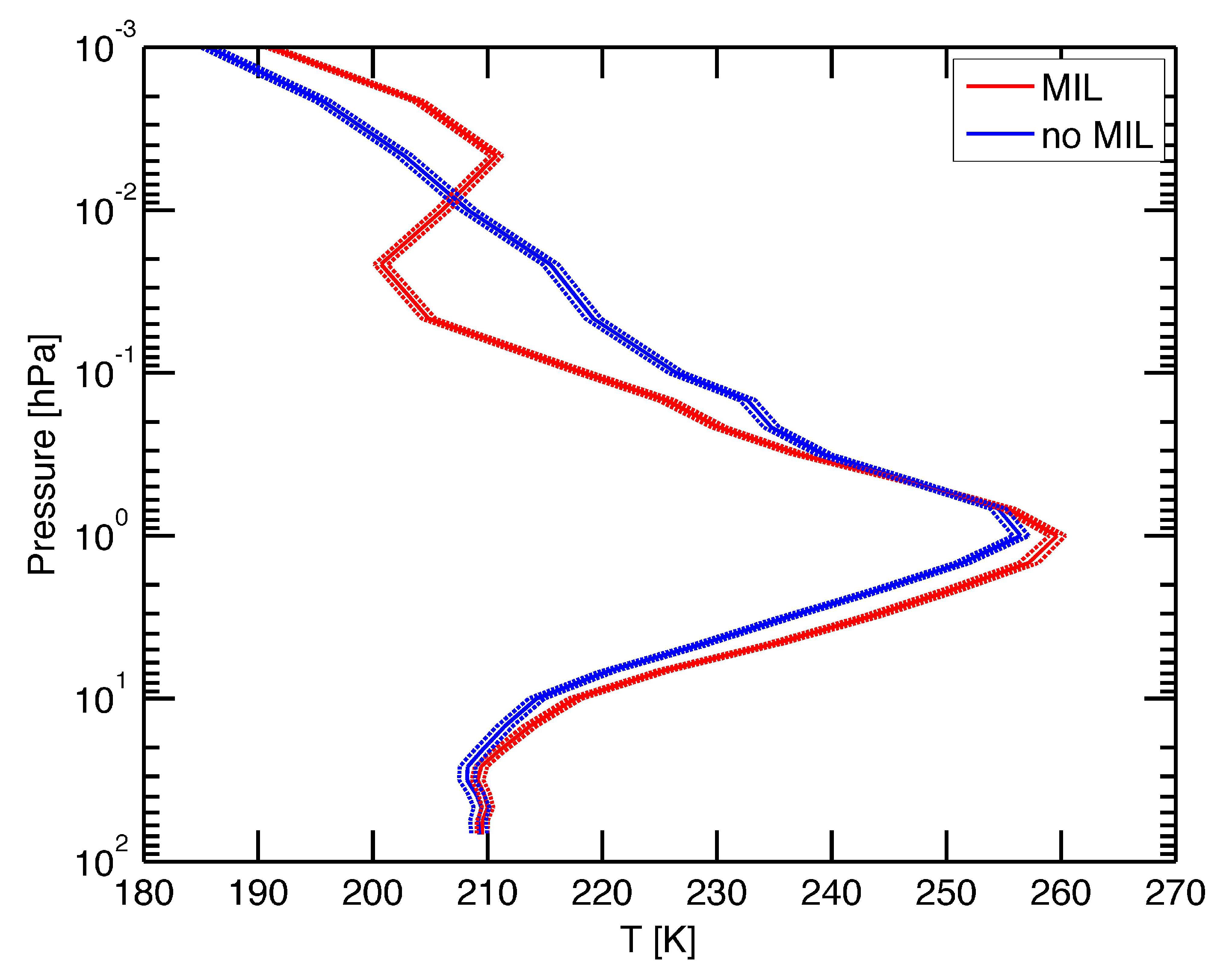
3.1. Mesospheric Inversion Layer above Bern

We start with a typical seasonal change of the vertical thermal state above Bern, Switzerland. Figure 1 shows the time series of daily temperature profiles from 1 October 2012 to 1 March 2013 observed by Aura/MLS above Bern. MILs are typically present at about p = 0.005 hPa (about 81 km) in the winter months from November to February. There was a major stratospheric sudden warming (SSW) on 6 January 2013 [25]. The major SSW was associated with a zonal wave-2 vortex splitting-pattern. About one week later, in mid January, an MIL occurs in Figure 1. Planetary wave-like oscillations with periods from 10 to 30 days usually occur in the wintertime stratosphere and mesosphere. The occurrence of planetary wave-like oscillations and MILs in Figure 1 indicates that MILs are generated by planetary waves in the wintertime at middle and high latitudes as it was previously shown by [2]. The maximum of the MILs occur on average at about 0.005 hPa (ca. 81 km), which is close to the value of [2], who reported an MIL height of 82 km derived for planetary wave-driven MILs in Aura/MLS data.

In the further analysis, we define two states and solely focus on daily average profiles observed above Bern in the winter months from December to February. The first state “MIL” happens when the temperature at 0.005 hPa is larger than the temperature at 0.025 hPa. This definition is in agreement with the definition of an inversion layer where the vertical temperature gradient changes from a negative sign to a positive sign. We do not use the MIL criterion of [2] who only considered strong MILs with a temperature increase of about 12 K in the mesosphere. The reason is that the MILs are not so strong over Europe and applying the strong criterion of [2] would lead to a poor statistics of observed MILs. The second state “no MIL” is fulfilled when the temperature at 0.005 hPa is lower than the temperature at 0.025 hPa. The MIL has an occurrence rate of 42%, which corresponds to 504 days with MIL out of 1205 winter days in total from 2004/2005 to 2017/2018. Figure 2 compares the mean temperature profiles of the two states. Because of the average over about 500 or 700 days, the error of the mean (denoted by the dotted lines) remains small. The red curve represents the state “MIL” and clearly shows a temperature maximum at about 0.005 hPa. The base of the MIL is at about 0.025 hPa where we can see that the “MIL” curve is about 15 K lower than the blue “no MIL” curve. The observation of a cold base of the MIL was also reported by [1]. Figure 3 shows the mean difference profile “MIL” minus “no MIL” for the temperature observations of Aura/MLS. In the middle and upper stratosphere, the temperature is increased by about 5–7 K larger during an MIL suggesting that an MIL is also connected to stratospheric changes in winter. Planetary wave propagation and breaking have a strong influence on the movements and deformations of the polar vortex in the stratosphere and the mesosphere [2]. Section 3.4 will analyse the displacement of the lower mesospheric polar vortex during an MIL.

Ref. [3] reported that planetary wave-driven MILs often occur above anticyclones. Thus, it makes sense to look at the difference profile of geopotential height (GPH) observed by Aura/MLS. Here, we use the temporal information of the two states and derive composites of GPH for the state “MIL” and for the state “no MIL”. The difference “MIL” minus “no MIL” is shown in Figure 4. The difference curve has a minimum at 0.01 hPa in the middle mesosphere and a maximum at 0.5 hPa in the lower mesosphere. In so far, the result of a pressure increase (anticyclone) below the “MIL” compared to “no MIL” in the lower mesosphere is in agreement with [3].

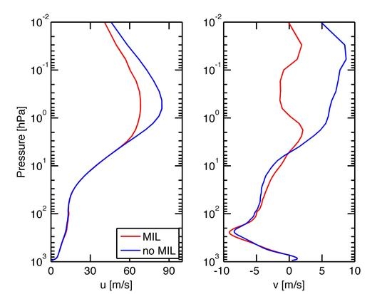
3.2. Coincident Changes in Horizontal Wind above Bern

The changes in zonal and meridional wind during an MIL are interesting, and they are investigated in this subsection. From ECMWF operational analysis, we derive the mean profiles for horizontal wind u and meridional wind v in case of “MIL” and “no MIL”. Figure 5 shows the clear result that the eastward wind in the lower mesosphere is slowed down by about 15 m/s when an MIL is present (red curve). Furthermore, the mesospheric northward wind v is slowed down from 5 m/s to zero when an MIL occurs. These results suggest that MILs are consequences of planetary wave breaking processes, which, in addition, are known to decelerate the horizontal mean flow. The westward traveling Rossby waves propagate against the eastward wind. In case of planetary wave breaking, the westward wave momentum is deposited to the eastward mean flow. In agreement with the deceleration of the eastward wind, the potential vorticity (from ECMWF) is slightly decreased in the winter mesosphere during MILs.

The vertical wind of ECMWF analysis shows no variation when MILs are present. However, the vertical wind is derived from the divergent component of the horizontal wind and is less reliable than the horizontal wind in meteorological reanalyses [26]. In addition, the mesospheric vertical wind is close to the top level ($p=0.01$ hPa) of the ECMWF model, which possibly reduces the accuracy of the vertical wind at mesospheric altitudes.

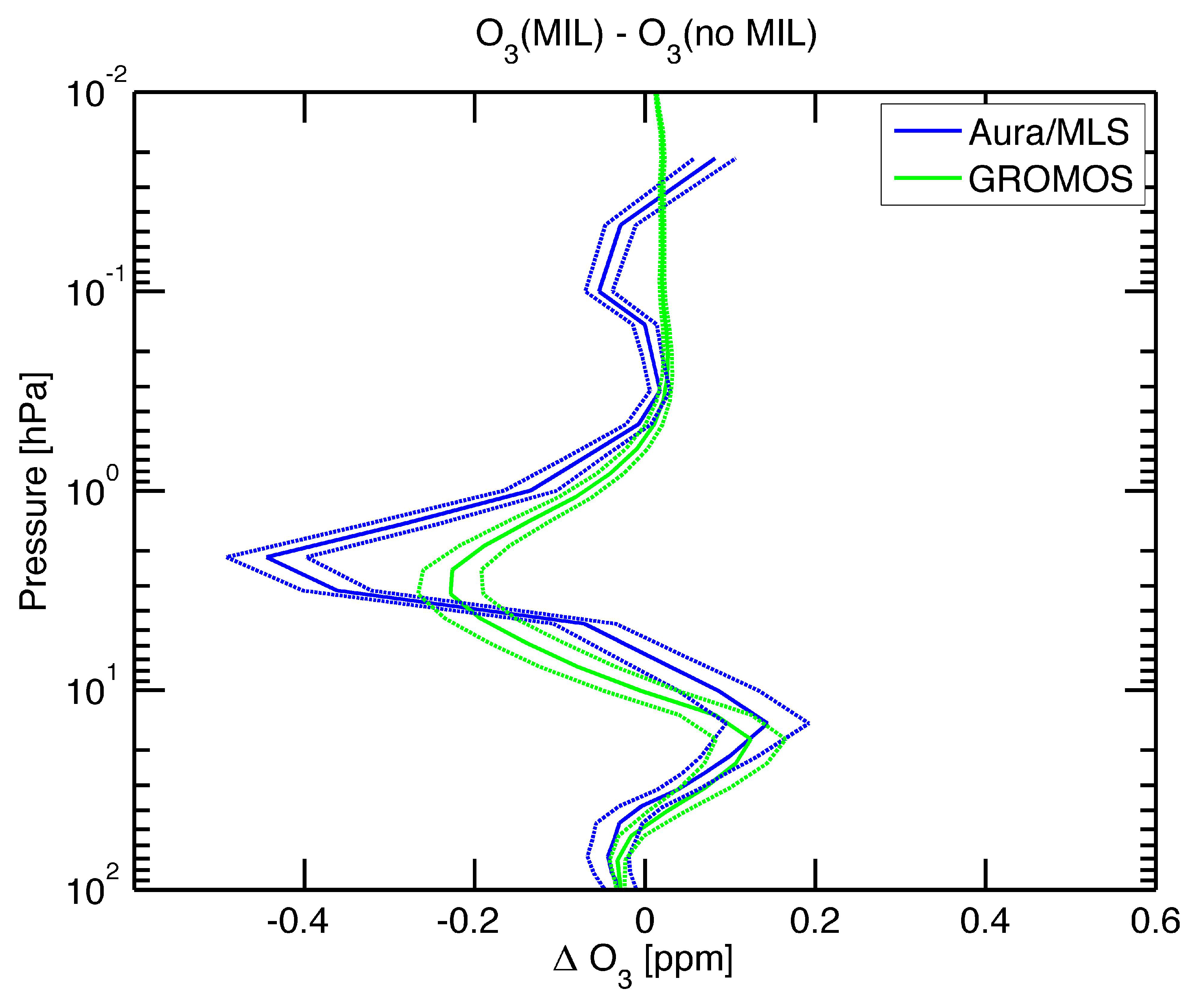
3.3. Coincident Changes in Ozone and Water Vapour above Bern

We derive the difference profiles “MIL” minus “no MIL” for the daily ozone observations of Aura/MLS and GROMOS at Bern. Figure 6 shows that upper stratospheric ozone is lowered by about 7% in case of Aura/MLS. The vertical resolution of GROMOS is lower than those of Aura/MLS. This explains the broader minimum of the upper stratospheric ozone in the green GROMOS curve. The contribution of the smoothing error is not included in the error bars of GROMOS, which are solely equal to the error of the mean. In the present study, the high resolution of Aura/MLS is kept since we do not want to lose information. Aura/MLS and GROMOS jointly show a decrease in upper stratospheric ozone when an MIL is present. It could be that the planetary wave disturbance shifts the polar vortex edge. On the other hand, the temperature (Figure 3) increases by about 5–7 K in the upper stratosphere during an MIL. The well-known anti-correlation of temperature and ozone in the upper stratosphere [27] seems to be the best explanation for the decrease of upper stratospheric ozone during an MIL. Ref. [28] found a relative decrease of 2.15% in an upper stratospheric ozone when the temperature increases by 1 K. Thus, the temperature change in Figure 3 is large enough to explain the 7% ozone decrease in Figure 6.

Using the daily averages of water vapour profiles from Aura/MLS (since 2004) and MIAWARA (since 2007) at Zimmerwald, we derive the difference profiles “MIL” minus “no MIL” for both instruments separately. Figure 7 shows the blue curve for Aura/MLS and the green curve for MIAWARA. Both curves show an increase in lower mesospheric water vapour at about 0.05 hPa (ca. 70 km) when an MIL is present. Because of its higher vertical resolution, Aura/MLS achieves a higher increase of about 20% in mesospheric water vapour during an MIL. Meridional advection of water vapour-rich air in the vicinity of the polar vortex edge could be an explanation since the life time of water vapour is about one month at 70 km altitude [29]. The $\Delta$H${}_2$O peak occurs at the same pressure level where the cold base of the MILs begins (Figure 2 and Figure 3). According to [2], the cold base of the MILs is related to local ascent and cooling situated atop the stratospheric anticyclones.

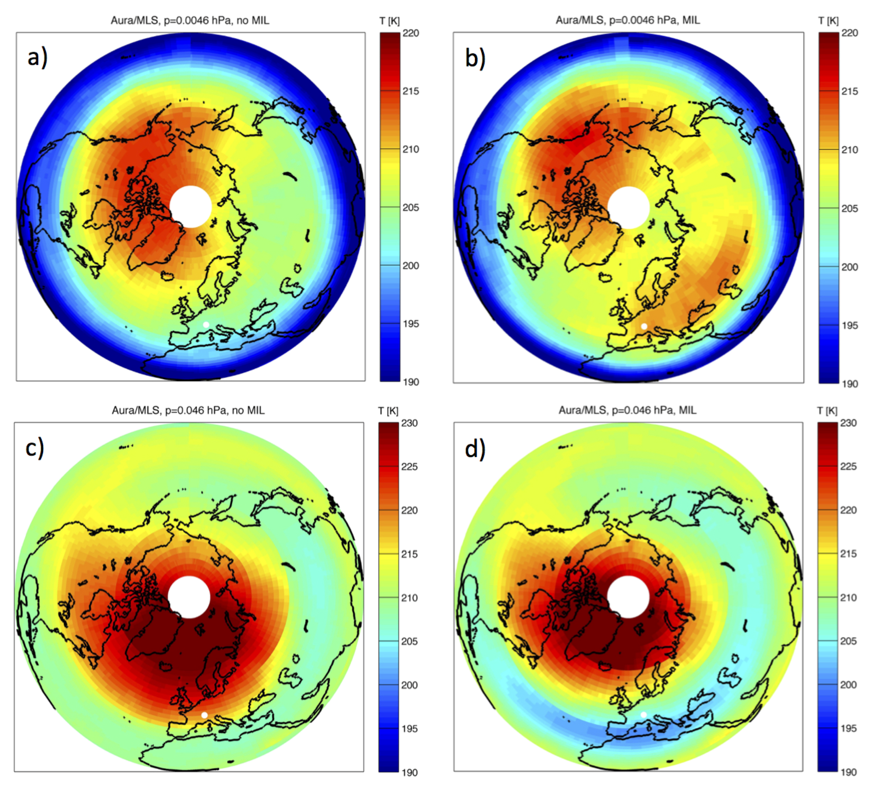
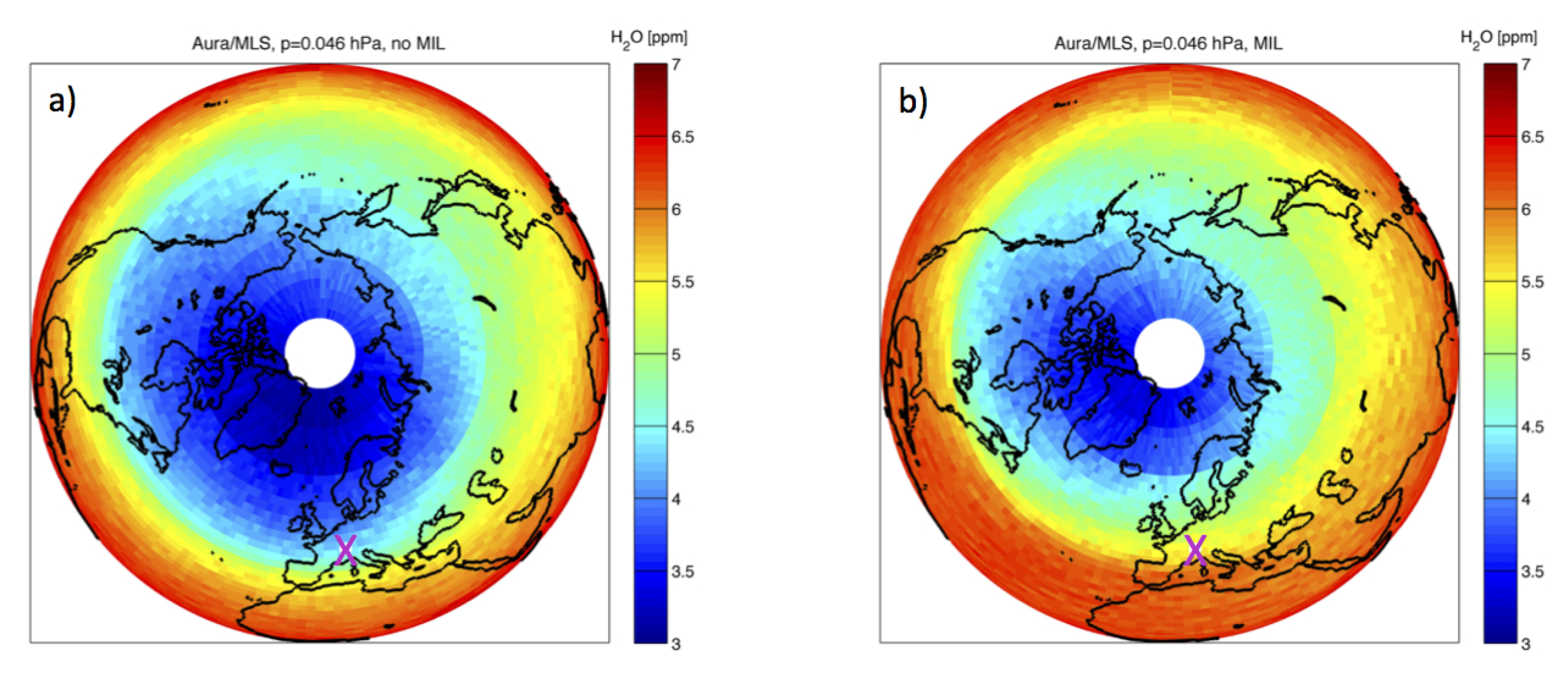
3.4. Northern Hemispheric Changes in Mesospheric Water Vapour and Temperature

The volume mixing ratio of water vapour is a good tracer for dynamics of the lower mesospheric vortex and the slow descent of dry air in the lower mesospheric polar vortex. The dry air is transported by the Brewer–Dobson circulation at upper mesospheric heights from low latitudes to the polar vortex where the air is descending [30]. Coincidently, the descending air is compressed at high latitudes in winter which explains the temperature increase at about 70 km altitude (0.046 hPa) in the polar mesosphere.

Figure 8 shows the change of the water vapour distribution at 0.046 hPa in the polar winter mesosphere depending on the occurrence of MILs. Figure 8a is the composite of the polar maps of Aura/MLS observations when the state “no MIL” is given at Bern, and Figure 8b shows the water vapour distribution when the state “MIL” occurs at Bern. The location of Bern is denoted by the magenta cross. It is evident that the increase of water vapour during an MIL is not a regional phenomenon, but it generally takes place at mid-latitudes. Furthermore, the blue area of dry air in the mesospheric polar vortex significantly decreases from the state “no MIL” to the state “MIL” in Figure 8. Especially, the blue area of dry air is shifted northward in the European longitude sector. Such a variation of the polar mesospheric water vapour distribution is explained by the dynamics of the polar vortex, which itself depends on planetary wave propagation from below.

In the case of the polar mesospheric temperature, we look at the pressure level of the MIL temperature peak, which is at 0.0046 hPa (about 82 km altitude). The composites at this level (Figure 9a,b) are compared to the composites at the cold base of the MIL (Figure 9c,d), which is at 0.046 hPa (about 70 km). Figure 9c,d nicely show how the warm air region of the polar vortex (reddish colours) is reduced when MILs occur above Bern. Similar to Figure 8, the vortex area is reduced in the European longitude sector so that the location of Bern, which is denoted by the small white dot turns from reddish colour in Figure 9c to bluish colour in Figure 9d. If one goes upward from the cold base (Figure 9d) to the MIL (Figure 9b), one can note that the location of Bern is inside a larger area of increased air temperature, which ranges from central Europe to Russia. This area of increased air temperature only occurs in the case when an MIL is above Bern. The other reddish area over North America and the Pacific occurs for both states “no MIL” and “MIL” in Figure 9a,b. We can state that the occurrence of an MIL above Bern is embedded in planetary-scale processes, which are related to deformations and movements of the polar mesospheric vortex in winter.

4. Conclusions

Our study is confined to weak MILs above central Europe that are present for periods of a day or longer. Generally, the study confirms the view that MILs at middle and high latitudes during winter are driven by planetary wave breaking [2]. In Bern (46.95${}^{\circ }$ N, 7.44${}^{\circ }$ E), the temperature peak of an MIL is in average at about 81 km height (0.005 hPa). In the winter months from December to February, the occurrence rate of an MIL is about 42% where we analysed Aura/MLS temperature data of 1205 winter days ranging from winter 2004/2005 to winter 2017/2018. The coincident changes in atmospheric composition and circulation during an MIL are a relative new branch of research. We find that the upper stratospheric ozone is reduced by about 7% during an MIL. This result is possibly due to the well-known anti-correlation between temperature and upper stratospheric ozone and the MIL-associated increase of upper stratospheric temperature. Furthermore, we find an increase of about 20% in lower mesospheric water vapour during an MIL. This result is possibly linked to the decrease of eastward and northward wind in the lower mesosphere during an MIL. The deceleration of the horizontal wind components during an MIL conforms with the idea that planetary wave breaking slows down the mean flow in the mesospheric surf zone. Finally, we find that the occurrence of an MIL above Bern is linked to deformations and movements of the mesospheric polar vortex in winter, which are visible in the distributions of water vapour and temperature as observed by Aura/MLS.

References

1. Meriwether, J.W.; Gerrard, A.J. Mesosphere inversion layers and stratosphere temperature enhancements. Rev. Geophys. 2004, 42. [Google Scholar] [CrossRef]
2. France, J.A.; Harvey, V.L.; Randall, C.E.; Collins, R.L.; Smith, A.K.; Peck, E.D.; Fang, X. A climatology of planetary wave-driven mesospheric inversion layers in the extratropical winter. J. Geophys. Res. Atmos. 2015, 120, 399–413. [Google Scholar] [CrossRef]
3. Sassi, F.; Garcia, R.R.; Boville, B.A.; Liu, H. On temperature inversions and the mesospheric surf zone. J. Geophys. Res. Atmos. 2002, 107. [Google Scholar] [CrossRef]
4. Salby, M.; Sassi, F.; Callaghan, P.; Wu, D.; Keckhut, P.; Hauchecorne, A. Mesospheric inversions and their relationship to planetary wave structure. J. Geophys. Res. Atmos. 2002, 107. [Google Scholar] [CrossRef]
5. Gan, Q.; Zhang, S.D.; Yi, F. TIMED/SABER observations of lower mesospheric inversion layers at low and middle latitudes. J. Geophys. Res. Atmos. 2012, 117, D07109. [Google Scholar] [CrossRef]
6. Schmidlin, F.J. Temperature inversions near 75 km. Geophys. Res. Lett. 1976, 3, 173–176. [Google Scholar] [CrossRef]
7. Hauchecorne, A.; Chanin, M.L.; Wilson, R. Mesospheric temperature inversion and gravity wave breaking. Geophys. Res. Lett. 1987, 14, 933–936. [Google Scholar] [CrossRef]
8. Leblanc, T.; Hauchecorne, A. Recent observations of mesospheric temperature inversions. J. Geophys. Res. Atmos. 1997, 102, 19471–19482. [Google Scholar] [CrossRef]
9. Irving, B.K.; Collins, R.L.; Lieberman, R.S.; Thurairajah, B.; Mizutani, K. Mesospheric Inversion Layers at Chatanika, Alaska (65 N, 147 W): Rayleigh lidar observations and analysis. J. Geophys. Res. Atmos. 2014, 119, 11235–11249. [Google Scholar] [CrossRef]
10. Liu, H.L.; Meriwether, J.W. Analysis of a temperature inversion event in the lower mesosphere. J. Geophys. Res. Atmos. 2004, 109. [Google Scholar] [CrossRef]
11. Liu, H.L.; Hagan, M.E.; Roble, R.G. Local mean state changes due to gravity wave breaking modulated by the diurnal tide. J. Geophys. Res. Atmos. 2000, 105, 12381–12396. [Google Scholar] [CrossRef]
12. Waters, J.W.; Froidevaux, L.; Harwood, R.S.; Jarnot, R.F.; Pickett, H.M.; Read, W.G.; Siegel, P.H.; Cofield, R.E.; Filipiak, M.J.; Flower, D.A.; et al. The Earth Observing System Microwave Limb Sounder (EOS MLS) on the Aura satellite. IEEE Trans. Geosci. Remote Sens. 2006, 44, 1075–1092. [Google Scholar] [CrossRef]
13. Schwartz, M.J.; Lambert, A.; Manney, G.L.; Read, W.G.; Livesey, N.J.; Froidevaux, L.; Ao, C.O.; Bernath, P.F.; Boone, C.D.; Cofield, R.E.; et al. Validation of the Aura Microwave Limb Sounder temperature and geopotential height measurements. J. Geophys. Res. Atmos. 2008, 113. [Google Scholar] [CrossRef] [Green Version]
14. Livesey, N.J.; Read, W.G.; Wagner, P.A.; Froidevaux, L.; Lambert, A.; Manney, G.L.; Millan Valle, L.F.; Pumphrey, H.C.; Santee, M.L.; Schwartz, M.J.; et al. Earth Observing System (EOS), Aura Microwave Limb Sounder (MLS), Version 4.2x Level 2 Data Quality and Description Document; Rep. JPL D-33509 Rev. C.; Jet Propulsion Laboratory: Pasadena, CA, USA, 2017.
15. ECMWF Model. Available online: https://www.ecmwf.int/en/research/modelling-and-prediction (accessed on 1 May 2018).
16. Dragani, R.; McNally, A.P. Operational assimilation of ozone-sensitive infrared radiances at ECMWF. Q. J. R. Meteorol. Soc. 2013, 139, 2068–2080. [Google Scholar] [CrossRef]
17. Rüfenacht, R.; Murk, A.; Kämpfer, N.; Eriksson, P.; Buehler, S.A. Middle-atmospheric zonal and meridional wind profiles from polar, tropical and midlatitudes with the ground-based microwave Doppler wind radiometer WIRA. Atmos. Meas. Tech. 2014, 7, 4491–4505. [Google Scholar] [CrossRef] [Green Version]
18. Eriksson, P.; Jimenez, C.; Buehler, S.A. Qpack, a general tool for instrument simulation and retrieval work. J. Quant. Spectrosc. Radiat. Transf. 2005, 91, 47–64. [Google Scholar] [CrossRef]
19. Eriksson, P.; Buehler, S.A.; Davis, C.P.; Emde, C.; Lemke, O. ARTS, the atmospheric radiative transfer simulator, version 2. J. Quant. Spectrosc. Radiat. Transf. 2011, 112, 1551–1558. [Google Scholar] [CrossRef]
20. Rodgers, C.D. Inverse Methods for Atmospheric Sounding—Theory and Practice; Series on Atmospheric Oceanic and Planetary Physics; World Scientific Publishing Co. Pte. Ltd.: Singapore, 2000; Volume 2. [Google Scholar]
21. Peter, R. The Ground-Based Millimeter-Wave Ozone Spectrometer—GROMOS; IAP Research Report 1997-13; Institut für Angewandte Physik, Universität Bern: Bern, Switzerland, 1997. [Google Scholar]
22. Moreira, L.; Hocke, K.; Eckert, E.; von Clarmann, T.; Kämpfer, N. Trend analysis of the 20-year time series of stratospheric ozone profiles observed by the GROMOS microwave radiometer at Bern. Atmos. Chem. Phys. 2015, 15, 10999–11009. [Google Scholar] [CrossRef] [Green Version]
23. Kämpfer, N.; Nedoluha, G.; Haefele, A.; De Wachter, E. Monitoring Atmospheric Water Vapour: Ground-Based Remote Sensing and In-Situ Methods; ISSI Scientific Report Series, Chapter Microwave Radiometry; Springer: New York, NY, USA, 2013; Volume 10, pp. 71–94. [Google Scholar]
24. Deuber, B.; Haefele, A.; Feist, D.G.; Martin, L.; Kämpfer, N.; Nedoluha, G.E.; Yushkov, V.; Khaykin, S.; Kivi, R.; Vömel, H. Middle Atmospheric Water Vapour Radiometer—MIAWARA: Validation and first results of the LAUTLOS/WAVVAP campaign. J. Geophys. Res. 2005, 110. [Google Scholar] [CrossRef]
25. Coy, L.; Pawson, S. The Major Stratospheric Sudden Warming of January 2013: Analyses and Forecasts in the GEOS-5 Data Assimilation System. Mon. Weather Rev. 2015, 143, 491–510. [Google Scholar] [CrossRef]
26. Kistler, R.; Kalnay, E.; Collins, W.; Saha, S.; White, G.; Woollen, J.; Chelliah, M.; Ebisuzaki, W.; Kanamitsu, M.; Kousky, V.; et al. The NCEP-NCAR 50-year reanalysis: Monthly means CD-ROM and documentation. Bull. Am. Meteorol. Soc. 2001, 82, 247–267. [Google Scholar] [CrossRef]
27. Froidevaux, L.; Allen, M.; Berman, S.; Daughton, A. The mean ozone profile and its temperature sensitivity in the upper stratosphere and lower mesosphere: An analysis of LIMS observations. J. Geophys. Res. Atmos. 1989, 94, 6389–6417. [Google Scholar] [CrossRef]
28. Schanz, A.; Hocke, K.; Kämpfer, N. Daily ozone cycle in the stratosphere: Global, regional and seasonal behaviour modelled with the Whole Atmosphere Community Climate Model. Atmos. Chem. Phys. 2014, 14, 7645–7663. [Google Scholar] [CrossRef] [Green Version]
29. Brasseur, G.P.; Solomon, S. Aeronomy of the Middle Atmosphere: Chemistry and Physics of the Stratosphere and Mesosphere, 3rd ed.; Springer: Dordrecht, The Netherlands, 2005; p. 644. [Google Scholar]
30. Straub, C.; Tschanz, B.; Hocke, K.; Kämpfer, N.; Smith, A.K. Transport of mesospheric H2O during and after the stratospheric sudden warming of January 2010: Observation and simulation. Atmos. Chem. Phys. 2012, 12, 5413–5427. [Google Scholar] [CrossRef] [Green Version]
Figure 1. Time series of daily temperature profiles above Bern, Switzerland from 1 October 2012 to 1 March 2013 observed by the Aura Microwave Limb Sounder. Mesospheric inversion layers (temperature enhancements) typically occur at about p = 0.005 hPa in the winter months from November to February. Planetary wave-like oscillations with periods from 10 to 30 days are present in the wintertime stratosphere and mesosphere. Dashed lines show the error of the mean.
Atmosphere 09 00171 g001
Figure 2. Composites of the temperature profile at Bern, Switzerland when the mesospheric inversion layer (MIL) is present (red) and when the MIL is absent (blue). All the winters (December to February) from 2004/2005 to 2017/2018 of Aura/MLS observations were used for the average temperature profiles. Dashed lines show the error of the mean.
Atmosphere 09 00171 g002
Figure 3. Temperature difference profile for “MIL” minus “no MIL”. A 5–7 K increase of temperature is present in the upper stratosphere at 2 hPa during an MIL. Dashed lines show the error of the mean.
Atmosphere 09 00171 g003
Figure 4. Geopotential height (GPH) difference profile for “MIL” minus “no MIL”. A relative increase of GPH (or pressure) is present in the lower mesosphere at 0.5 hPa when an MIL occurs. Dashed lines show the error of the mean.
Atmosphere 09 00171 g004
Figure 5. ECMWF (European Centre for Medium-range Weather Forecast) analysis at Bern: Eastward wind u and northward wind v during an MIL (red) and during “no MIL” (blue). Dashed lines show the error of the mean.
Atmosphere 09 00171 g005
Figure 6. Difference profiles “MIL” minus “no MIL” for ozone observations by the ground-based ozone radiometer GROMOS (green) and by the satellite experiment Aura/MLS (blue) above Bern during winter. Dashed lines show the error of the mean.
Atmosphere 09 00171 g006
Figure 7. Difference profiles “MIL” minus “no MIL” for water vapour observations by MIAWARA (green) and by Aura/MLS (blue) above Bern during winter. Dashed lines show the error of the mean.
Atmosphere 09 00171 g007
Figure 8. Polar plots of mesospheric water vapour at p = 0.046 hPa (at cold base of MIL and at peak of water vapour change at Bern) observed by Aura/MLS during winter: (a) composite when “no MIL” was above Bern; (b) composite when an “MIL” was above Bern. The location of Bern is indicated by the magenta cross.
Atmosphere 09 00171 g008
Figure 9. Polar plots of mesospheric temperature observed by Aura/MLS during winter: (a) composite at p = 0.0046 hPa when “no MIL” was above Bern; (b) composite at p = 0.0046 hPa (at MIL peak) when an “MIL” was above Bern; (c) composite at p = 0.046 hPa when “no MIL” was above Bern; (d) composite at p = 0.046 hPa (at cold base) when an “MIL” was above Bern. The location of Bern is indicated by the small white dot.
Atmosphere 09 00171 g009