FY-3A Microwave Data Assimilation Based on the POD-4DEnVar Method

Abstract

A four-dimensional ensemble variational assimilation system for FY-3A satellite data is constructed using the Proper Orthogonal Decomposition (POD)-based ensemble four-dimensional variational (4DVar) assimilation method (referred to as POD-4DEnVar Satellite Assimilation System). Using the community radiative transfer model (CRTM) as the observation operator for satellite data, ensemble samples are mapped to the observation space and observation perturbations are generated. The observation perturbations matrix of satellite data is then decomposed to obtain the orthogonal eigenvectors and the eigenvalues for the observation perturbations matrix. The observation perturbations matrix and model perturbations matrix are transformed using orthogonal eigenvectors as basis functions and an explicit expression for the analysis increment is obtained. The expression includes the flow-dependent background error covariance and avoids the difficulty of solving the adjoint model for four-dimensional variational assimilation. In order to evaluate the capability of POD-4DEnVar Satellite Assimilation System, single observation experiments and observation system simulation experiments (OSSEs) for FY-3A MWHS and MWTS sensor data were designed to simulate a large-scale precipitation event occurring over the middle and lower reaches of the Yangtze River. The results of single observation experiments show that POD-4DEnVar Satellite Assimilation System can assimilate satellite data correctly, and the background error covariance of POD-4DEnVar Satellite Assimilation System has obvious flow-dependent characteristics. The results of the OSSEs show that the root-mean-square errors (RMSEs) of the assimilation analysis field with respect to the “true” field are lower than those of the background field, which indicates that the POD-4DEnVar Satellite Assimilation System can assimilate satellite data effectively. The sensitivity of the POD-4DEnVar Satellite Assimilation System to the percentage of truncated eigenvalues, the number of ensemble members, assimilation time window length, and the horizontal localization scale (which are key parameters for POD-4DEnVar Satellite Assimilation System) was tested in sensitivity experiments. These experiments show that if the percentage of truncated eigenvalues for POD decomposition is more than 80%, POD-4DEnVar Satellite Assimilation System has strong assimilation skill. Increasing the number of initial ensemble members has little influence on the assimilation ability of POD-4DEnVar Satellite Assimilation System. But, increasing the number of the physical ensemble members can clearly increase the assimilation ability. The assimilation skill of POD-4DEnVar Satellite Assimilation System is optimal when the length of the assimilation time window is 5 h or 3 h and the horizontal localization scale is 500 km or above. The assimilation ability of POD-4DEnVar Satellite Assimilation System is preliminarily tested by single observation experiments and OSSEs. The results show that it is feasible to assimilate satellite data using the POD-4DEnVar method. In the future, a variety of real satellite data and a variety of mesoscale weather cases will be used to further verify the stability of POD-4DEnVar Satellite Assimilation System.

1. Introduction

Satellite observations play a very important role in improving the accuracy of mesoscale weather forecasts [1]. At present, most assimilation studies for satellite data adopt a variational method. The four-dimensional variational (4DVar) method uses a model as a constraint to assimilate observations at multiple times in the assimilation window. Bias corrections are easy to implement by using the variational framework, so many operational numerical weather forecasting centers adopt the 4DVar method for satellite data assimilation [2]. However, the adjoint model solution of 4DVar requires a lot of computational resources, which limits its development. At the same time, the ensemble Kalman filter (EnKF) based ensemble assimilation method can construct flow-dependent background error covariance without requiring the solution of the tangent linear adjoint model [3,4,5]. As a result, methods of ensemble assimilation for satellite data have been developed, such as ensemble square-root filtering [6,7], ensemble transform Kalman filtering, and local ensemble transform Kalman filtering [8,9]. However, the limited number of ensemble members for the ensemble assimilation method can cause large sample errors, so both 4DVar and EnKF assimilation methods have their own advantages and disadvantages. In order to avoid the shortcomings of 4DVar and EnKF, a four-dimensional ensemble hybrid assimilation method (4DEnVar) is proposed [10]. Qiu et al. proposed using the singular value decomposition (SVD) method in order to construct the base vector of analyzing increments [11]. The cost function is transformed into an explicit expression on control variables and there is no need to solve the adjoint and tangent linear model. Liu et al. proposed a 4DEnVar assimilation method using ensemble perturbations directly as a basis vector [12,13,14]. Wang et al. developed a 4DVar assimilation method (DRP-4DVar) while using dimension-reduced projection [15]. This method performs EOF decomposition on ensemble perturbations and it reduces the dimensionality by selecting EOF modes. Good experimental results have been obtained in Lorenz96 mode, Observing System Simulation Experiments (OSSEs), and assimilation experiments for real observations [16,17,18].

Tian et al. proposed a variational four-dimensional ensemble assimilation method, based on Proper Orthogonal Decomposition (POD) [19]. Similar to Liu et al.’s method [12], the method combines variational assimilation and an ensemble Kalman filter that not only makes the background error covariance flow-dependent, but also avoids the problem of solving the adjoint and tangent linear model of 4DVar. Testing on the Lorenz system, the shallow water wave equation and the global chemical transport model Geos-Chem show that this method has great potential for applications [19,20,21]. It is found that the PODEn4DVar outperforms both the 4DVar and the EnKF under both perfect and imperfect-model scenarios with lower computational costs than the EnKF [19]. At present, the Proper Orthogonal Decomposition (POD)-based ensemble three-dimensional variational (3DVar) assimilation method (referred to as POD-3DEnVar) and POD-4DEnVar assimilation systems that are based on radar data have been developed successfully [22,23]. Assimilation experiments show that the systems can effectively improve the description of dynamic and microphysical characteristics for the initial convective field, and thus effectively increase the capability for precipitation forecast. At present, most of the data assimilated by the POD-4DEnVar method are radar data, and there has been no previous study of an application of this method to assimilate satellite data, specifically the Chinese FY-satellite data. The wide coverage and high spatial resolution of satellite data mean that they are widely used in numerical weather forecasting. Satellite data, especially microwave sensor data, can effectively improve the initial field of numerical forecasts. The successful launch of the Chinese polar orbiting meteorological satellite FY-3A on 27 May 2008 with its Microwave Humidity Sounder (MWHS) and Microwave Temperature Sounder (MWTS) have provided the vertical profiles of atmospheric temperature and humidity that are important for numerical weather forecasting. It provides an important source of vertical atmospheric satellite sounding data for use in regional and global assimilation systems [24]. Therefore, the assimilation and application of FY-satellite data has attracted much attention. The assimilation of FY-satellite data into the WRF model with the advanced POD-4DEnVar method could improve the accuracy of the numerical forecast.

As the first attempt to assimilate FY-3A MWHS and MWTS with the POD-4DEnVar assimilation method, the community radiative transfer model (CRTM) is used here as an observational operator for the satellite data. Using initial and physical ensemble forecasting samples to construct ensemble perturbations [25,26,27], single observation experiments and observation system simulation experiments are carried out for a large-scale precipitation event over the middle and the lower reaches of the Yangtze River.

The article is organized as follows. The second section briefly introduces the theoretical framework of POD-4DEnVar. In the third section, the key technologies of POD-4DEnVar in satellite data assimilation are analyzed and the POD-4DEnVar Satellite Assimilation System is established. The fourth section describes rainstorm cases and model parameter settings. The results of single observation experiments, OSSEs are analyzed in the fourth section. The fifth section analyzes the results of sensitivity experiments for the percentage of truncated eigenvalue, the number of ensemble members, the length of assimilation time window, and the horizontal localization scale in the system. The robustness of POD-4DEnVar Satellite Assimilation System and the optimal settings of the relevant sensitivity parameters are tested. The sixth section provides a summary.

2. Introduction to the POD-4DEnVar Method

The following is a brief introduction to the mathematical framework of POD-4DEnVar. For a detailed derivation, see the article by Tian et al. [19]. The cost function of the incremental form for 4DVar is:

$$J(x^{\prime })=\frac{1}{2}{(x^{\prime })}^{\mathrm{T}}{B}^{-1}(x^{\prime })+\frac{1}{2}{\displaystyle \sum _{t=0}^{s-1}{\left[y_t^{\prime }(x^{\prime })-(y_t^{obs}{)}^{\prime }\right]}^{\mathrm{T}}{R}_t^{-1}\left[y_t^{\prime }(x^{\prime })-(y_t^{{}^{obs}}{)}^{\prime }\right]}$$

(1)

In Formula (1), $t$ indicates the observation times in the assimilation time window, $s$ indicates the total number of observational times in the assimilation window. Superscript $\mathrm{T}$ indicates the transpose of a matrix, and ${\mathbf{B}}^{-1}$ and $R_t^{-1}$ are the inverses of the background and observation error covariance matrices at time $t$, respectively. $x^{\prime }$ is the analysis increment at $t=0$, $y_t^{\prime }(x^{\prime })$ is the observed increment at time $t$, $(y_t^{{}^{obs}}{)}^{\prime }$ is the observed innovation at time $t$, and the specific expressions for each item are:

$$x^{\prime }=x-x_b,t=0$$

(2)

$$y_t^{\prime }(x^{\prime })=y_t({\mathbf{x}}_b+x^{\prime })-y_t({\mathbf{x}}_b),\mathrm{t}=0,1,2,\cdots ,s-1$$

(3)

$$y_t(\mathrm{x})=H_t\left({\mathit{M}}_{0\to t}\right(\mathbf{x}\left)\right),\mathrm{t}=0,1,2,\cdots ,s-1$$

(4)

$$(y_t^{obs}{)}^{\prime }=(y_t^{obs})-y_t({\mathbf{x}}_b),\mathrm{t}=0,1,2,\cdots ,s-1$$

(5)

Here, ${\mathbf{H}}_t$ represents the observation operator at time $t$ in the above formula, ${\mathit{M}}_{0\to t}$ indicates that the forecast model integrates from initial time to observation time $t$ and ${\mathbf{y}}_t^{obs}$ represents the observation at time $t$, $x_b$ is the background field.

POD-4DEnVar solves the cost function (1) without solving the adjoint and the tangent linear model. The specific approach is as follows.

First, $N$ ensemble members are given at time $t$. The ensemble members can reflect the uncertainty of initial field at time $t$. $N$ ensemble forecasting members $({\mathbf{x}}_1,{\mathbf{x}}_2,\cdots ,{\mathbf{x}}_N)$ can generate $N$ ensemble forecast perturbations $\left(x_1^{\prime },x_2^{\prime },\cdots ,x_N^{\prime }\right)$ to the background field $x_b$, where ${\mathbf{x}}_i^{\prime }={\mathbf{x}}_i-{\mathbf{x}}_b$ $(i=1,2,\cdots ,N)$. We call it the model perturbations (MPs) matrix, which is defined as the $X^p$. By mapping $N$ ensemble forecasting perturbations into observation space through the observation operator $H$, $N$ observation perturbations can be generated. Over the $s$ observation times in the assimilation time window, $N\times s$ observation perturbations $({\mathbf{y}}_{1,t}^{\prime },{\mathbf{y}}_{2,t}^{\prime },\cdots ,{\mathbf{y}}_{N,t}^{\prime }),t=0,1,2,\cdots ,s-1$ can be generated that define the observation perturbations (OPs) matrix $Y^p$.

After using the ensemble members to form the MPs matrix, it is assumed that analysis increment ${\mathbf{x}}^{\prime }$ can be approximately linearly related to the model perturbations, and then ${\mathbf{x}}^{\prime }$ can be expressed as the linear weighted sum of ensemble perturbations in $({\mathbf{x}}_1^{\prime },{\mathbf{x}}_2^{\prime },\dots ,{\mathbf{x}}_N^{\prime })$ space, namely:

$${\mathbf{x}}^{\prime }={\mathsf{\beta }}_1{\mathbf{x}}_1^{\prime }+{\mathsf{\beta }}_2{\mathbf{x}}_2^{\prime }+\cdots +{\mathsf{\beta }}_N{\mathbf{x}}_N^{\prime }$$

(6)

where ${\mathsf{\beta }}_1,{\mathsf{\beta }}_2\cdots ,{\mathsf{\beta }}_N$ are the linear combination coefficients. Writing:

$${\mathsf{\beta }=(\mathsf{\beta }}_1,{\mathsf{\beta }}_2\cdots ,{\mathsf{\beta }}_N{)}^T$$

(7)

then:

$${\mathbf{x}}^{\prime }=x^p\mathsf{\beta }$$

(8)

Replacing the (8) formula into the cost function of (1) form, the solution to the incremental ${\mathbf{x}}^{\prime }$ is transformed to the solution of the linear combination coefficient $\mathsf{\beta }$. Because the dimension of the linear combination coefficient $\mathsf{\beta }$ is much smaller than the dimension of the increment ${\mathbf{x}}^{\prime }$, the amount of calculation is greatly reduced.

In order to make ensemble members have better independent representation. Since the dimension of the observed variable space is much smaller than the dimension of model space [15], the POD decomposition is performed on the OPs matrix $Y^p$ [28,29]:

$$Y^p{}^T{Y}^p=V{\Lambda }^2{V}^{\mathrm{T}}$$

(9)

where $\Lambda :\left({\Lambda }_1,{\Lambda }_2,{\Lambda }_3\cdots {\Lambda }_{\mathrm{N}}\right)$ and $V:\left(V_1,V_2,V_3\cdots V_{\mathrm{N}}\right)$ are the decomposed eigenvalues and eigenvectors, respectively. $V:\left(V_1,V_2,V_3\cdots V_{\mathrm{N}}\right)$ is an orthogonal matrix. The eigenvectors are used as the basis function to transform the OPs matrix. They are usually truncated when transforming the OPs matrix. The first $\mathrm{M}$ eigenvalues $\left({\Lambda }_1,{\Lambda }_2,{\Lambda }_3\cdots {\Lambda }_{\mathrm{M}},\mathrm{M}\le \mathrm{N}\right)$ that represent the main features of the OPs matrix are selected from $\left({\Lambda }_1,{\Lambda }_2,{\Lambda }_3\cdots {\Lambda }_{\mathrm{N}}\right)$.

We define the POD-transformed OPs matrix:

$$P_y=Y^{p}V$$

(10)

Here, $V:\left(V_1,V_2,V_3\cdots V_{\mathrm{M}}\right)$ are the eigenvectors corresponding to the eigenvalues after the truncation. ${\mathbf{P}}_y$ is the OPs matrix after transformation, and ${\mathbf{P}}_y$ is independent of each other. From (2) to (4), it can be seen that the OPs originate from the MPs. Therefore, after the transformation of the OPs matrix $Y^p$, the MPs matrix $X^p$ should also be transformed accordingly. If we assume that there is a linear relationship between the MPs matrix $X^p$ and the OPs matrix $Y^p$, we can transform the model forecast increment $X^p$, as follows:

$${\mathbf{P}}_x=X^p\mathbf{V}$$

(11)

where ${\mathbf{P}}_x$ is the transformed independent MPs matrix.

The optimal solution ${\mathbf{x}}^{\prime }$ and its corresponding model equivalent ${\mathbf{y}}^{\prime }$ in observation space can be expressed by the linear combinations of the POD-transformed MPs and OPs, respectively, as follows:

$${\mathbf{x}}^{\prime }={\mathbf{P}}_x\mathsf{\beta }$$

(12)

and

$${\mathbf{y}}^{\prime }={\mathbf{P}}_y\mathsf{\beta }$$

(13)

Substituting (12), (13), and the ensemble background covariance $B=\frac{P_x{P}_x{}^T}{N-1}$ into (1), the control variable becomes $\mathsf{\beta }$ instead of ${\mathbf{x}}^{\prime }$, so the control variable is expressed explicitly in the cost function:

$$J(\mathsf{\beta })=\frac{1}{2}(N-1)\cdot {\mathsf{\beta }}^T{P}_x^T{\left(P_x^T\right)}^{-1}{\left(P_x\right)}^{-1}{P}_x\mathsf{\beta }+\frac{1}{2}{\left(P_y\mathsf{\beta }-y_{\mathrm{obs}}^{\prime }\right)}^T{R}^{-1}\left(P_y\mathsf{\beta }-y_{obs}^{\prime }\right)$$

(14)

Through simple calculations (see Tian et al. [19] for more details), the explicit expression for the analysis increment is:

$$x_{}^{\prime }=P_x{\left[(N-1)I+P_y^T{R}^{-1}{P}_y\right]}^{-1}{P}_y^T{R}^{-1}{y}_{obs}^{\prime }$$

(15)

As an ensemble-based assimilation scheme, the localisation strategy is essential to ameliorate the spurious long-range correlations resulting from the limited number of ensemble members [30]. In the POD-4DEnVar method, we use the following filter function as the horizontal correlation model [31]:

$${\mu }_h={\mathbf{C}}_0(d_x/d_{x,0})·{\mathbf{C}}_0(d_y/d_{y,0})$$

(16)

$${\mathbf{C}}_0(r)=\{\begin{array}{ll}-\frac{1}{4}{r}^5+\frac{1}{2}{r}^4+\frac{5}{8}{r}^3-\frac{5}{3}{r}^2+1,& 0\le r\le 1\\ \frac{1}{12}{r}^5-\frac{1}{2}{r}^4+\frac{5}{8}{r}^3+\frac{5}{3}{r}^2-5r+4-\frac{2}{3}{r}^{-1},& 1<r\le 2\\ 0,& 2<r\end{array}$$

(17)

In Formula (16), ${\mu }_h$ represents the horizontal localization coefficient. $d_x$ and $d_y$ are the zonal and meridional distances between the observation point and model grid point, respectively. $d_{x,0}$ and $d_{y,0}$ are the zonal and meridional localization radius, respectively. ${\mathbf{C}}_0(r)$ is the localization correlation function, which is related to the distance between the model point and the observation point. Following Zhang et al. [32], vertical localization is performed using the correlation function,

$${\mu }_v(\Delta \log P)=\frac{1}{1+5\times {(\Delta \log P)}^2}$$

(18)

in which $\Delta \log P$ is the distance between two vertical levels in $\log P$ space, and $P$ is air pressure.

With the horizontal and vertical localization scheme, the final POD-4DEnVar analysis increment ${\mathbf{x}}^{\prime }$ in Equation (15) is formulated using the Schur product, as follows:

$$x_a=x_b^{}+({\mathsf{\mu }}_h\cdot {\mathsf{\mu }}_v)\circ \left\{P_x{\left[(N-1)I+P_y^T{R}^{-1}{P}_y\right]}^{-1}{P}_y^T{R}^{-1}{y}_{obs}^{\prime }\right\}$$

(19)

${\mathsf{\mu }}_h$ and ${\mathsf{\mu }}_v$ represent horizontal and vertical localization vectors, respectively. The Schur product of two matrices having the same dimension is denoted by $A=B\circ C$, and it consists of the element-wise product, such that $a_{ij}=b_{ij}\cdot c_{ij}$.

3. Application of the POD-4DEnVar Method in Satellite Data Assimilation

From the principles of POD-4DEnVar, we know that the key to the method for satellite data assimilation is the construction of the OPs matrix $Y^p$ and the POD decomposition. The observation operator $H$ must be used in calculating simulated observations. Because brightness temperature is not a forecast variable of the numerical model, the observation operator is a complex radiative transfer model. The CRTM radiative transfer model is one of the most widely used rapid radiative transfer models in satellite data assimilation [33]. The CRTM can calculate satellite brightness temperature quickly and accurately, and thus it is very suitable for application to the satellite data assimilation system. Observations from Microwave Humidity Sounder (MWHS) and Microwave Temperature Sounder (MWTS) onboard Fengyun-3A can provide the vertical information of atmospheric temperature and humidity, which is very important to the numerical weather forecast. The MWHS contain five channels, mainly using the water vapor absorption band to detect the vertical humidity structure of the atmosphere. The MWTS contain four channels, mainly using the oxygen absorption band to detect the vertical temperature structure of the atmosphere. The center frequency and weighting function peak height of FY3A-MWHS and MWTS are displayed in

Table 1. Channel characteristics of FY-3A Microwave Humidity Sounder (MWHS) and Microwave Temperature Sounder (MWTS).

Sensor	Channel Number	Center Frequency (GHz)	Weighting Function Peak Height (hPa)
MWHS	1	150(V)	Surface
	2	150(H)	Surface
	3	183.31 + 1(H)	400
	4	183.31 + 3(H)	600
	5	183.31 + 7(H)	800
MWTS	1	50.30(V)	Surface
	2	53.596 + 0.115(H)	700
	3	54.94(V)	300
	4	57.29(H)	90

. The remote sensing information of these channels contains more information about the humidity and temperature of the atmosphere. Through simulating the brightness temperature of each channel of MWHS and MWTS by CRTM, the observation perturbations matrix is constructed, and POD-4DEnVar Satellite Assimilation System is constructed.

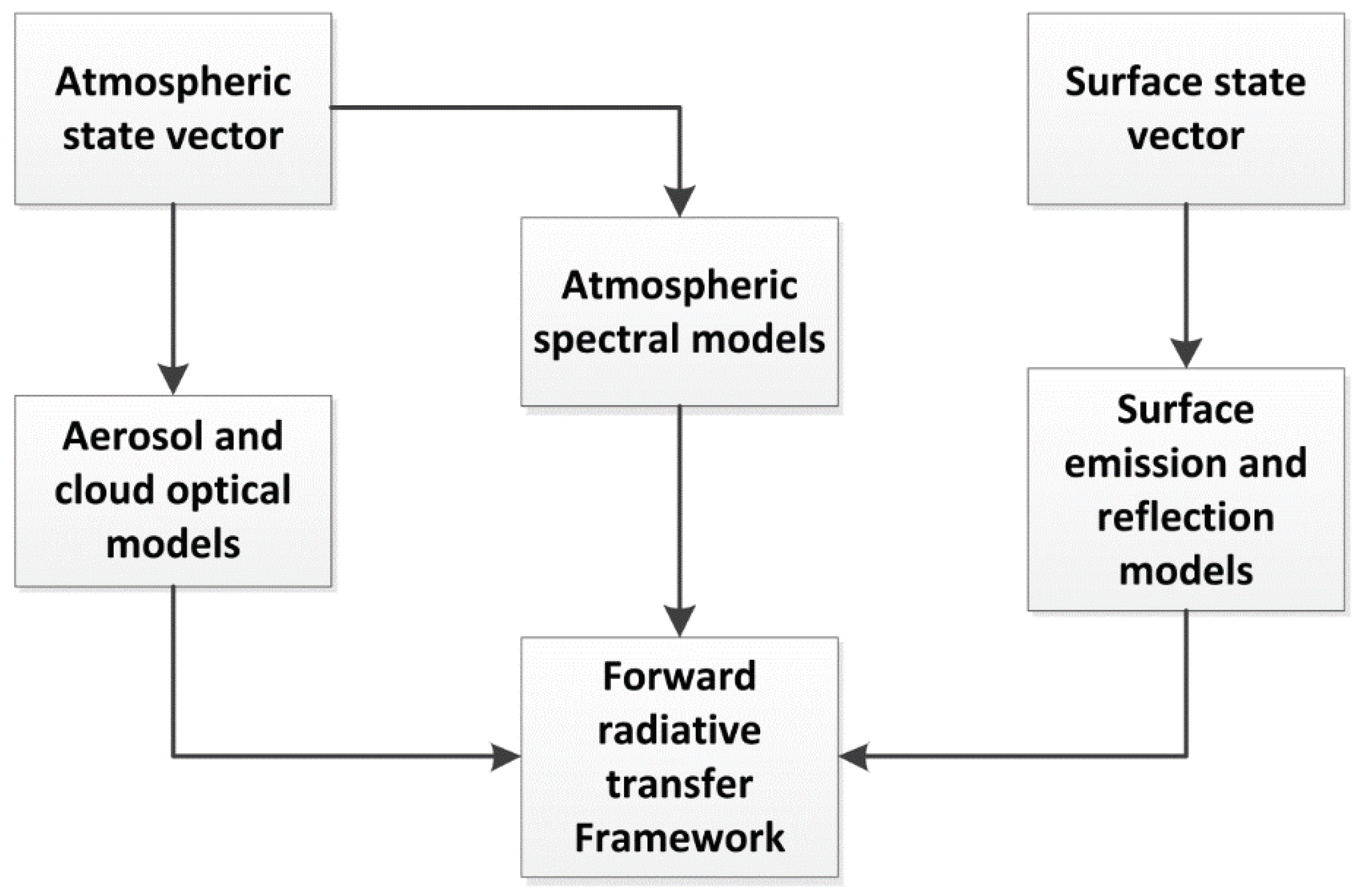
Figure 1 shows the composition of the CRTM radiative transfer model. First, we need to provide the atmospheric state vector, including the atmospheric temperature and humidity profile and the surface state vector as input fields. The optical thickness of the atmospheric absorption components is calculated with an atmospheric spectral model, and the absorption and scattering of clouds and aerosols are also considered when they affect observations. Atmospheric downward radiation interacts with the earth’s surface and the surface emissivity is calculated by an emission-reflection model for the earth’s surface. By integrating atmospheric absorption, cloud and aerosol absorption, and scattering optical coefficients, the atmospheric transmissivity is calculated. Inputting atmospheric transmissivity and surface emissivity into the forward radiative transfer model, the satellite brightness temperatures can be simulated. Therefore, by mapping ensemble perturbations to observation space through the CRTM model, the OPs matrix in the assimilation window can be obtained. This process is critical to the implementation of POD-4DEnVar Satellite Assimilation System.

Figure 2 shows the flowchart of the POD-4DEnVar Satellite Assimilation System. The first step is ensemble forecasting that produces ensemble forecasting samples in the assimilation window. The second step is to map the ensemble forecasting members into observation space through the CRTM model to produce the OPs. Then, the OPs matrix is constructed in the assimilation window. The third step is to perform POD decomposition on the OPs matrix to obtain decomposed eigenvalues and eigenvectors. The eigenvalues are truncated and the corresponding major eigenvectors are obtained. The OPs matrix is transformed according to the major eigenvectors to obtain the independent OPs matrix. At the same time, the MPs matrix is also transformed according to the eigenvectors in order to obtain the independent the MPs matrix. The fourth step is to plug the transformed OPs matrix, the transformed MPs matrix and the observation innovation $(y_t^{obs}{)}^{\prime }$ into the Formula (1). This gives an explicit expression of the analysis increment. Horizontal and vertical localizations are then calculated for the analysis increment, and finally, the localized analysis increment is added to the background field to obtain the analysis field. Note that before the real satellite data are introduced into the POD-4DEnVar assimilation system, they should be preprocessed, including channel selection, quality control, thinning, and bias correction.

4. Assimilation Experiments

4.1. Precipitation Case Studies and Model Settings

A large-scale strong precipitation event occurred over the middle and lower reaches of the Yangtze River from 00:00 UTC on 29 June 2009 to 00:00 UTC on 30 June 2009. Figure 3 shows the 24 h accumulated observed precipitation distribution that was initiated at 00:00 UTC on 29 June 2009. In most areas of rainfall, the precipitation is between 100 and 150 mm. Three heavy rainstorm cores above 100 mm 24 h⁻¹ are located in southern Anhui, northeastern Hubei, and western Hubei. The maximum 24 h precipitation in southern Anhui and southwestern Hubei are more than 200 mm. Precipitation cores are located in Huaining in Anhui (241.5 mm 24 h⁻¹) and Hefeng in Hubei (313.2 mm 24 h⁻¹).

The WRF model version 3.6 is used as the forecasting model in the POD-4DEnVar Satellite Assimilation System. The experiments were conducted over a 180 × 120 grid mesh with a grid spacing of 30 km and 27 vertical layers. The model top is at 50 hPa. The main physical components of the WRF model that was used in our experiments include the WSM6 microphysical scheme [34], the Kain-Fritsch cumulus parameterization scheme [35], the RRTM longwave radiation scheme [36], the Dudhia shortwave radiation scheme [37], the YSU boundary layer scheme [38], and the Noah LSM land-based scheme [39]. The NCEP Final (FNL) Operational Model Global Tropospheric Analyses 1° × 1° (http://dss.ucar.edu/datasets/ds083.2/matrix.html) were used as the first-guess field and the boundary conditions in the experiments. The analysis time of the assimilation experiments is valid at 00:00 UTC on 29 June 2009. The variables that were updated in the assimilation include u, v, and w winds, perturbation temperature, perturbation pressure, water-vapor mixture ratio, and rainwater mixing ratio.

4.2. Construction of Ensemble Samples

The ensemble samples are based on the 12 h forecast fields of 50 members from the TIGGE ECMWF ensemble forecasting products (http://apps.ecmwf.int/datasets/data/tigge/). Using the ensemble forecast products as initial fields, the 12 h forecast fields are generated hour by hour. The results of three times (23:00 UTC on 28 June 2009, 00:00 UTC on 29 June 2009, and 01:00 UTC on 29 June 2009) are used as the ensemble forecast samples, giving 150 ensemble samples [40]. In order to make the ensemble samples more representative, physical ensemble samples are also included in the ensemble samples for assimilation [26,27,28]. Using the different planetary boundary layer schemes, microphysical schemes, and cumulus parameterization schemes in the WRF model, 18 physical ensemble samples are generated; the specific combinations of schemes are shown in

Table 2. Physical ensemble forecast schemes.

The Number of Physical Ensemble Member	The Physical Ensemble Scheme
	The Planetary Boundary Layer Schemes	The Microphysical Schemes	The Cumulus Parameterization Schemes
1	MRF [41]	Kessler [42]	Kain-Fritsch [43]
2	MRF	Kessler	Betts-Miller-Janjic [44]
3	MRF	Kessler	Grell-Freitas [45]
4	MRF	Lin et al. [46]	Kain-Fritsch
5	MRF	Lin et al.	Betts-Miller-Janjic
6	MRF	Lin et al.	Grell-Freitas
7	MRF	Lin et al.	Kain-Fritsch
8	MRF	Lin et al.	Betts-Miller-Janjic
9	MRF	Lin et al.	Grell-Freitas
10	YSU [38]	Kessler	Kain-Fritsch
11	YSU	Kessler	Betts-Miller-Janjic
12	YSU	Kessler	Grell-Freitas
13	YSU	Lin et al.	Kain-Fritsch
14	YSU	Lin et al.	Betts-Miller-Janjic
15	YSU	Lin et al.	Grell-Freitas
16	YSU	Eta [47] microphysics	Kain-Fritsch
17	YSU	Eta microphysics	Betts-Miller-Janjic
18	YSU	Eta microphysics	Grell-Freitas

. The physical ensemble samples are produced from the 12 h forecast field initiated at 12:00 UTC on 28 June 2009. Therefore, the total number of ensemble samples used in the experiment is 168.

4.3. Single Observation Experiments

4.3.1. Experimental Design

The single observation experiment only uses the data of FY-3A MWHS channel 5. The assimilation time is 00:00 UTC on 29 June 2009 (i.e., the midpoint of the assimilation window). The length of the assimilation time window is 7 h, from 20:30 UTC on 28 June 2009 to 03:30 UTC on 29 June 2009. Then, the single observation is placed on the point (31.71° N, 116.81° E) near the storm rainfall center in southern Anhui, which is marked by the red star in Figure 4. The vertical height of the single observation is 800 hPa, corresponding to the peak height of MWHS channel 5. The simulated brightness temperature of the background field is 267 K at the single-observation location. Two experiments were designed to test the effect of assimilation (

Table 3. Design of single observation experiments.

Experiments Name	Single Observation Tb	Simulated Tb	The Location of Single Observation
SOE1	264 K	267 K	31.71° N, 116.81° E 800 hPa
SOE2	270 K	ditto	ditto

). The satellite brightness temperature in the single observation experiment 1 (SOE1) is 264 K, which is lower than that of the background field. The brightness temperature in the single observation experiment 2 (SOE2) is 270 K, which is higher than that of the background field. Therefore, the observation in SOE1 and SOE2 are synthetic. The localization scale is 300 km. The 168 ensemble samples are used and the eigenvalues are not truncated for the two single observation experiments.

4.3.2. Analysis of Results

Figure 4 shows the increments of SOE1 for the 500 hPa horizontal wind field, vertical velocity, 700 hPa temperature, rainwater mixing ratio, and relative humidity. In the figure, the 500 hPa horizontal wind increments (Figure 4a) show obvious cyclonic convergence and the vertical velocity increments (Figure 4b) are positive, which are in good agreement with the large precipitation cores. The temperature increments at 700 hPa (Figure 4c) have significant positive values in the precipitation area. The rainwater mixing ratio increments (Figure 4d) and the relative humidity increments at 700 hPa (Figure 4e) are also mainly positive in the precipitation area. Along the 31° N meridional-vertical section (not shown), positive increments of vertical velocity extend from the surface to the top, while the positive increments of rainwater mixing ratio are mainly distributed near the surface. When POD-4DEnVar Satellite Assimilation System assimilates a brightness temperature 3 K below the background field, the horizontal wind convergence is effectively strengthened. This increases vertical velocity and rainwater mixing ratio and enhances the convection. Figure 4 also shows that the increments of SOE1 are non-uniform and anisotropic. The horizontal wind increments converge around the single observation location, and the vertical velocity increments are mainly located in the precipitation cores. The increments of rainwater mixing ratio and temperature also reflect the non-uniform and the anisotropic characteristics of the environmental wind field.

The analysis increments of SOE2 (figure not shown) are opposite to those of SOE1. The horizontal wind increments diverge and negative increments of vertical velocity are mainly found in the precipitation cores. At the same time, the increments of temperature, rainwater mixing ratio, and the relative humidity are mainly negative in the precipitation cores. The increments of vertical velocity and rainwater mixing ratio along the 31° N meridional-vertical section (not shown) are negative. The results of SOE1 and SOE2 show that the POD-4DEnVar successfully assimilates a single observation from satellite data. The construction of the POD-4DEnVar Satellite Assimilation System is successful. It is feasible to assimilate satellite data using the POD-4DEnVar method. The background error covariance for POD-4DEnVar method has flow-dependent characteristics.

4.4. Observation System Simulation Experiments

4.4.1. Experimental Design

Observing system simulation experiments (OSSEs) were designed to further investigate the ability of assimilating satellite data by the POD-4DEnVar method. The effectiveness of the assimilation method can be assessed by comparing the RMSEs between the analysis field and the “true” field.

The simulated satellite observations include data from the five channels of FY-3A MWHS and the four channels of MWTS. The location and time of the simulated observations are consistent with the real observations. Two assimilation analysis time were designed to test the effect of assimilation. The first assimilation analysis time is 00:00 UTC on 29 June 2009. The second assimilation analysis time is 12:00 UTC on 29 June 2009. In order to remove the effect of spin-up, the simulated observations are constructed, as follows. The 12 h forecast fields that were initialized at 12:00 UTC on 28 June 2009 and 00:00 UTC on 29 June 2009 are regarded as the “true” field for the two assimilation analysis time. The “true” field is used as the input to the CRTM radiative transfer model, and the simulated brightness temperatures at the assimilation time are obtained. The assimilation analysis time is located at the midpoint of the assimilation window. The length of the assimilation time window is 7 h. The first assimilation time window is from 20:30 UTC on 28 June 2009 to 03:30 UTC on 29 June 2009. The second assimilation time window is from 08:30 UTC on 29 June 2009 to 15:30 UTC on 29 June 2009. The background fields over the first assimilation time window are provided by the forecasting fields that are initialised using the FNL data from 18:00 UTC on 28 June 2009 with the WRF model, in which the first 6 h are taken as the spin-up period. The background fields over the second assimilation time window are provided by the 12 h forecasting fields that are initialised using assimilation analysis field at the first assimilation time.

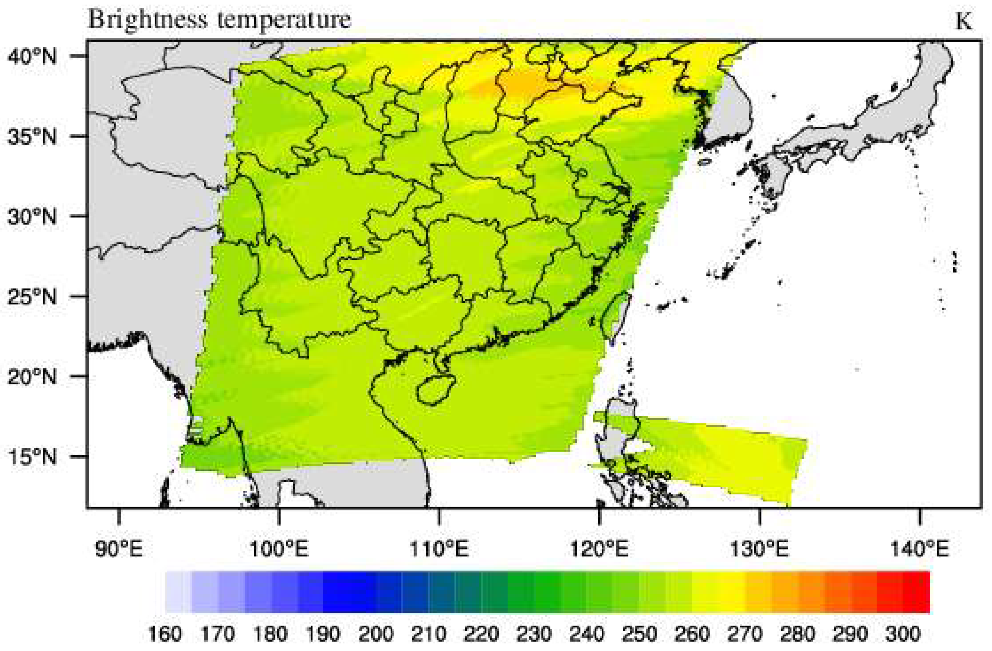
Figure 5 shows the simulated brightness temperature distribution of channel 4 of FY-3A MWHS in the first assimilation time window. The background is the model domain. The simulated MWHS brightness temperatures sweep through most of the model domain and completely cover Anhui and Hubei provinces where precipitation occurs. When assimilating the simulated observations, there is no need for bias correction and quality control, and only thinning is performed, with a thinning scale of 60 km. The number of simulated observations that were assimilated in the first assimilation time window and the second assimilation time window were 23,332 and 15,621, respectively.

In order to test the assimilation effect of the POD-4DEnVar Satellite Assimilation System, three experiments (

Table 4. Design of observation system simulation experiments (OSSEs).

Experiments Name	Assimilation Method	Experiments Purposes
Con	None	Comparative experiment
POD-3DEnVar	POD-3DEnVar	Test the effect of POD-3DEnVar on assimilation
POD-4DEnVar	POD-4DEnVar	Test the effect of POD-4DEnVar on assimilation

) were designed in the OSSEs. Experiment Con did not assimilate any observation data. The POD-3DEnVar experiment assimilated the simulated observation data in the assimilation time window, but the total number of observation times s is 1, which is equivalent to POD-based three-dimensional variational assimilation. The observation data at the assimilation time window are considered as the observations that are valid at the analysis time. The POD-4DEnVar experiment assimilated the simulated observation data over the assimilation time window, and the total number of observation times s is 7. The simulated observations are given hour by hour. In the experiments of POD-3DEnVar and POD-4DEnVar, the eigenvalues are not truncated. The localization scale is 1500 km. The 168 ensemble samples are used in the experiments.

4.4.2. Analysis of OSSE Results

It is well known that the Root Mean Square Error (RMSE) is defined in Formula (20). In the OSSEs, the RMSEs between the analysis field and “true” field were used to assess the effect of the assimilation experiments. The smaller the RMSEs, the better the assimilation effect. Figure 6 shows the vertical profiles of RMSEs for u winds, v winds, temperature, water vapor mixing ratio, and relative humidity for Con, POD-3DEnVar, and POD-4DEnVar. The assimilation analysis results are valid at 00:00 UTC on 29 June 2009.The RMSEs of POD-3DEnVar for the four variables are smaller than those of Con, and the RMSEs of POD-4DEnVar for the four variables are lower again than those of POD-3DEnVar, which shows that both POD-4DEnVar and POD-3DEnVar can effectively assimilate satellite observations and that the assimilation ability of POD-4DEnVar is significantly stronger than that of POD-3DEnVar.

$$RMSE=\sqrt{\frac{{\displaystyle {\sum }_{i=1}^n{\left(X_{true,i}-X_{analysis,i}\right)}^2}}{n}}$$

(20)

Figure 7 shows the vertical profiles of RMSEs for u winds, v winds, temperature, water vapor mixing ratio, and relative humidity for Con, POD-3DEnVar, and POD-4DEnVar. The assimilation analysis results are valid at 12:00 UTC on 29 June 2009. Similar to Figure 6, the RMSEs of POD-3DEnVar for the four variables are generally smaller than those of Con, and the RMSEs of POD-4DEnVar for the four variables are generally lower again than those of POD-3DEnVar. This further demonstrates the assimilation ability of POD-4DEnVar.

The analysis fields derived from the assimilation and the “true” field at two assimilation analysis times that were obtained in Section 4.4.1 are used as the initial fields for 12 h forecasts. Figure 8 shows the evolution of the RMSEs of the 24 h forecast field of cycling assimilation for Con, POD-3DEnVar, and POD-4DEnVar. As the integration time increases, the RMSEs of the forecast fields for Con gradually increase. But, the RMSEs of the forecast fields for POD-3DEnVar and POD-4DEnVar do not increase significantly with the increase of integration time. The RMSEs of POD-3DEnVar are smaller than those of Con, and the RMSEs of POD-4DEnVar are smaller than those of POD-3DEnVar. This further demonstrates that POD-4DEnVar Satellite Assimilation System can effectively assimilate satellite observations and improve the accuracy of the 24 h forecast field. It also shows that the POD-4DEnVar assimilation method has a significant improvement when compared with the POD-3DEnVar method.

5. Sensitivity Experiments for the Key Parameters of POD-4DEnVar

5.1. Eigenvector Truncation Number for POD Decomposition

5.1.1. Experimental Design

The POD decomposition is an important process in the POD-4DEnVar Satellite Assimilation System. Eigenvalues are usually truncated when transforming the OPs by eigenvectors. The first M eigenvalues $\left({\Lambda }_1,{\Lambda }_2,{\Lambda }_3\cdots {\Lambda }_M,M\le N\right)$ that represent the main features of the OPs matrix are selected from $\left({\Lambda }_1,{\Lambda }_2,{\Lambda }_3\cdots {\Lambda }_N\right)$. The principle is to keep the variance contribution of eigenvalues and reduce the computational cost. Define $k=({\Lambda }_1+{\Lambda }_2+{\Lambda }_3+\cdots +{\Lambda }_M)/({\Lambda }_1+{\Lambda }_2+{\Lambda }_3+\cdots +{\Lambda }_N)\times 100\%$ as the percentage of truncated eigenvalues. To reveal the effect of k on assimilation, five experiments were designed with k values of 100%, 96%, 92%, 83%, and 56% (

Table 5. Experimental design for eigenvector truncation sensitivity.

Experiments Name	The Values of M	The Percentage of Truncated Eigenvalues k	Assimilation Methods
Con			None
Exp1_1	168	100%	POD-4DEnVar
Exp1_2	98	96%	POD-4DEnVar
Exp1_3	68	92%	POD-4DEnVar
Exp1_4	51	83%	POD-4DEnVar
Exp1_5	3	56%	POD-4DEnVar

). The assimilation used POD-4DEnVar in the five experiments. The assimilation time is 00:00 UTC on 29 June 2009 (i.e., the midpoint of the assimilation window). The length of the assimilation time window is 7 h. The localization scale is 1500 km. The 168 ensemble samples are used in the experiments. The simulated observations that were used in the experiments are the same as the experiment POD-4DEnVar in Section 4.4. The experiment Con with no assimilation is also the same as Con in Section 4.4.

5.1.2. Analysis of Results

Figure 9 shows the vertical profiles of the RMSEs for u winds, v winds, temperature, water vapor mixing ratio, and relative humidity from the Con, Exp1_1, Exp1_2, Exp1_3, Exp1_4, and Exp1_5. As k decreases gradually, the RMSEs of the analysis field gradually increase. When k is 100%, the RMSEs of the analysis field are obviously smaller than that of other experiments. When comparing the results of Exp1_2, Exp1_3, and Exp1_4, there are little difference between the results of the experiments. This shows that when k are 96%, 92%, and 83%, it has little influence on the assimilation results. When k is 56%, the RMSEs of the analysis field are obviously higher, and are close to Con. Therefore, the result of assimilation is optimal when k is 100%. In order to ensure the assimilation effect and minimize the cost of computation, k should be more than 80%.

5.2. Number of Ensemble Members

5.2.1. Experimental Design

In the POD-4DEnVar method, the number N of ensemble members $({\mathbf{x}}_1,{\mathbf{x}}_2,\cdots ,{\mathbf{x}}_N)$ affects the size of the OPs and MPs matrix, which affects the result of POD decomposition and the effect of assimilation. For practical application, in order to save computing resources, we should try to reduce the number of ensemble samples while ensuring the quality of the assimilation. For this reason, sensitivity experiments were designed to reveal the effect of N on the assimilation. In the experiments, values of 50, 68, 100, 150, and 168 are used for the number $N$ of ensemble members. The assimilation time is 00:00 UTC on 29 June 2009 (i.e., the midpoint of the assimilation window). The length of the assimilation time window is 7 h. The localization scale is 1500 km. The eigenvalues are not truncated. The simulated observations used in the assimilation are the same as POD-4DEnVar in Section 4.4. Con is also the same as experiment Con in Section 4.4. The experimental design is shown in

Table 6. Experimental design for ensemble size sensitivity experiments.

Experiments Name	The Number of Ensemble Members N	Assimilation Methods
Con		None
Exp2_1	50 (50 TIGGE Ensemble)	POD-4DEnVar
Exp2_2	68 (50 TIGGE Ensemble + 18 Physical Ensemble)	POD-4DEnVar
Exp2_3	100 (100 TIGGE Ensemble)	POD-4DEnVar
Exp2_4	150 (150 TIGGE Ensemble)	POD-4DEnVar
Exp2_5	168 (150 TIGGE + 18 Physical Ensemble)	POD-4DEnVar

. The numbers of ensemble members for Exp2_1, Exp2_3, and Exp2_4 are 50, 100, and 150, respectively. Exp2_1 used 50 TIGGE ECMWF ensemble forecast products at 00:00 UTC on 29 June 2009. Based on 50 TIGGE ECMWF ensemble forecast products in Exp2_1, Exp2_2 added 18 physical ensemble forecast samples to 68 samples. Exp2_3 used 50 TIGGE ECMWF ensemble forecast products at 23:00 UTC on 28 June 2009 and 50 TIGGE ECMWF ensemble forecast products at 00:00 UTC on 29 June 2009. Therefore, 100 ensemble samples were used in the experiment2_3. Exp2_4 used 50 TIGGE ECMWF ensemble forecast products at 23:00 UTC on 28 June 2009 and 50 TIGGE ECMWF ensemble forecast products at 00:00 UTC on 29 June 2009 and 50 TIGGE ECMWF ensemble forecast products at 01:00 UTC on 29 June 2009. Therefore, 150 ensemble samples were used in the experiment2_4. Based on 150 TIGGE ECMWF ensemble forecast products in Exp2_4, Exp2_5 added 18 physical ensemble forecast samples to 168 samples.

5.2.2. Analysis of Results

Figure 10 shows the vertical profiles of the RMSEs in u winds, v winds, temperature, water vapor mixing ratio, and relative humidity from the Con, Exp2_1, Exp2_2, Exp2_3, Exp2_4, and Exp2_5. The RMSEs of each variable in Exp2_5 are significantly smaller than those of other experiments. As $N$ decreases, the RMSEs of the analysis field increase. However, the RMSEs of each variable in Exp2_2 are smaller than those of Exp2_3 and Exp2_4, which indicates that the physical ensemble members have a more obvious effect on assimilation than initial ensemble members. Therefore, it is very important to use physical ensemble members in the assimilation process. When comparing the results of Exp2_1, Exp2_3, and Exp2_4, there are little difference between the results of experiments that only contain the initial ensemble.

5.3. Length of Assimilation Window

5.3.1. Experimental Design

The length of the assimilation time window is also an important parameter for POD-4DEnVar Satellite Assimilation System. Define $L$ as the actual length in hours of the assimilation time window. If $L$ is too long, then the cost of computation will be significantly increased. If $L$ is too short, the observed data assimilated into POD-4DEnVar Satellite Assimilation System will be relatively reduced. Therefore, four sensitivity experiments were designed to reveal the effect of $L$ on assimilation. In the experiments, $L$ are 1 h, 3 h, 5 h, and 7 h. The analysis time is at the midpoint of the assimilation time window. The localization scale is 1500 km. The 168 ensemble samples are used in the experiments. The eigenvalues are not truncated. The simulated observations used in the assimilation are the same as the experiment POD-4DEnVar in Section 4.4. Con is also the same as experiment Con in Section 4.4. The specific experimental design is shown in

Table 7. Experimental design for assimilation window sensitivity experiments.

Experiments Name	The Length of Assimilation Window L	Assimilation Methods
Con		None
Exp3_1	1 h	POD-4DEnVar
Exp3_2	3 h	POD-4DEnVar
Exp3_3	5 h	POD-4DEnVar
Exp3_4	7 h	POD-4DEnVar

.

5.3.2. Analysis of Results

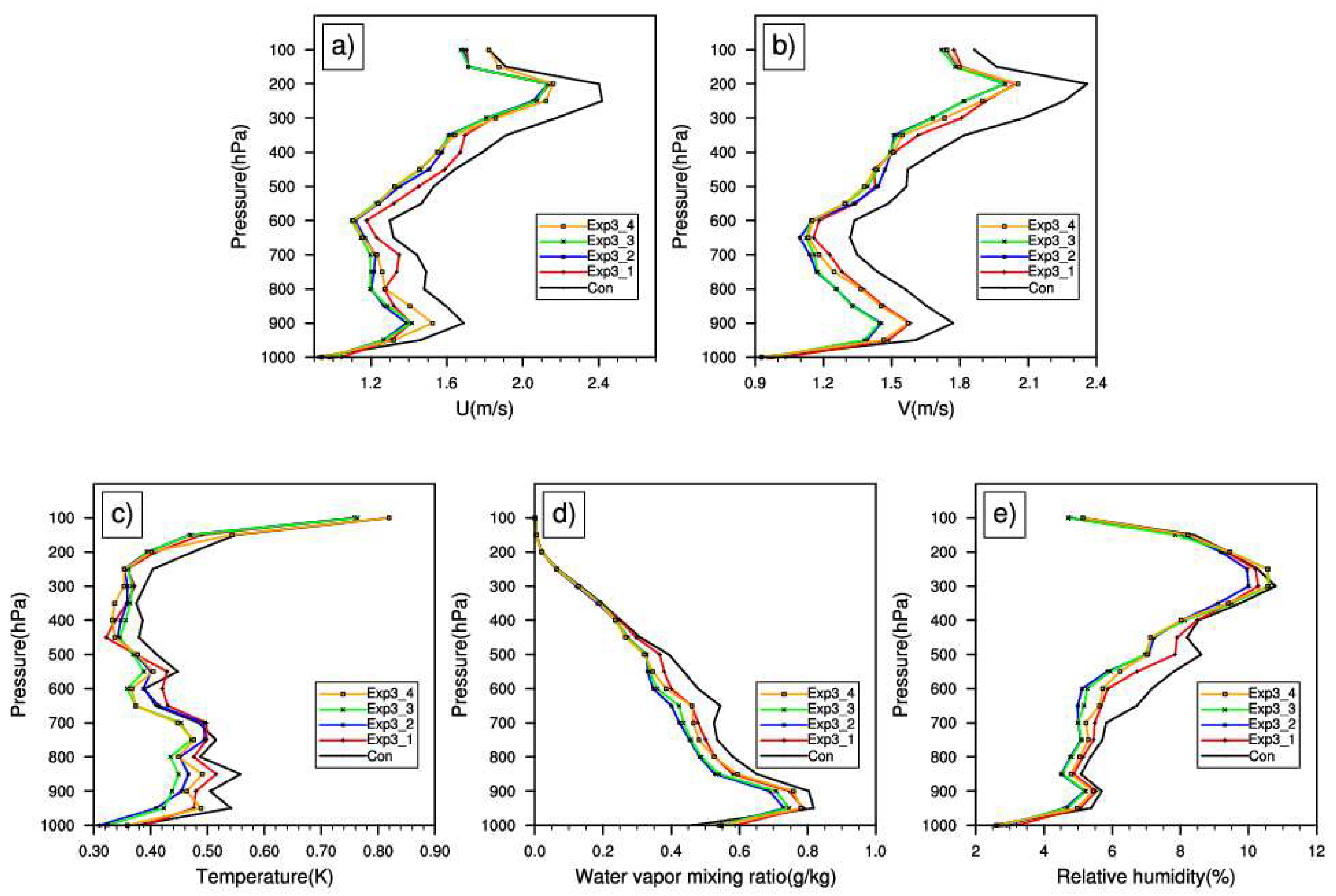
Figure 11 shows the vertical profiles of RMSEs in u winds, v winds, temperature, water vapor mixing ratio, and relative humidity from the Con, Exp3_1, Exp3_2, Exp3_3, and Exp3_4. The RMSEs of each variable in Exp3_3 and Exp3_2 are relatively small. The RMSEs of Exp3_4 are larger than those of Exp3_3. Since the assimilation time window is too short, the analysis field of Exp3_1 has a significantly larger RMSEs. However, the RMSEs of analysis fields for all experiments are significantly lower than those of Con. These sensitivity experiments show that the optimal assimilation time window length is 5 h or 3 h.

5.4. Horizontal Localization Scale

5.4.1. Experimental Design

In the POD-4DEnVar method, the localisation strategy is essential to ameliorate the spurious long-range correlations resulting from the limited number of ensemble members. Define $R=\sqrt{d_{x,0}{}^2+d_{y,0}{}^2}$ as the horizontal localization scale. Therefore, five sensitivity experiments are designed to reveal the effect of $R$ on assimilation. In the experiments, $R$ are 50 km, 100 km, 500 km, 1000 km, and 1500 km. The assimilation time is 00:00 UTC on 29 June 2009 (i.e., the midpoint of the assimilation window). The length of the assimilation time window is 7 h. The 168 ensemble samples are used and the eigenvalues are not truncated in the experiments. The simulated observations that were used in the assimilation are the same as the experiment POD-4DEnVar in Section 4.4. Con is also the same as experiment Con in Section 4.4. The specific experimental design is shown in

Table 8. Experimental design for horizontal localization scale.

Experiments Name	The Horizontal Localization Scale R	Assimilation Methods
Con		None
Exp4_1	50 km	POD-4DEnVar
Exp4_2	100 km	POD-4DEnVar
Exp4_3	500 km	POD-4DEnVar
Exp4_4	1000 km	POD-4DEnVar
Exp4_5	1500 km	POD-4DEnVar

.

5.4.2. Analysis of Results

Figure 12 shows the vertical profiles of the RMSEs in u winds, v winds, temperature, water vapor mixing ratio, and relative humidity from the Con, Exp4_1, Exp4_2, Exp4_3, Exp4_4, and Exp4_5. When comparing the results of Exp4_5, Exp4_4, and Exp4_3, there are little differences between the results of experiments. This shows that when R is 500 km and above, it has little influence on assimilation results. When R is less than 500 km, the RMSEs of the analysis field begin to decrease. When R is 50 km, the RMSEs are closer to those of Con. Therefore, the horizontal localization scale R should be 500 km or above.

6. Conclusions

Using the POD-4DEnVar assimilation method, the POD-4DEnVar Satellite Assimilation System was constructed to assimilate FY-3A satellite data. The CRTM radiative transfer model is the observation operator for satellite data that is used to map the ensemble samples to observation space. Observation perturbations are generated and are then decomposed to obtain the orthogonal eigenvectors and eigenvalues. The orthogonal eigenvectors are used as the basis functions to transform the observation perturbations matrix and model perturbations matrix, and an explicit expression of the analysis increment is obtained. The expression includes flow-dependent background error covariance and avoids the difficulty of solving the adjoint model for four-dimensional variational assimilation. In order to evaluate the capability of POD-4DEnVar Satellite Assimilation System, single observation experiments and observation system simulation experiments for FY-3A MWHS and MWTS sensor data were designed for a large-scale precipitation event occurring over the middle and lower reaches of the Yangtze River. The results of the single observation experiments show that the POD-4DEnVar Satellite Assimilation System can assimilate satellite data correctly, and the background error covariance of POD-4DEnVar Satellite Assimilation System has obvious flow-dependent characteristics. The results of the OSSEs show that the RMSEs of the analysis field for assimilation experiments with the “real” field are less than those of the background field, which indicates that the POD-4DEnVar Satellite Assimilation System can assimilate satellite data effectively. The sensitivity of POD-4DEnVar Satellite Assimilation System to key parameters, including the percentage of truncated eigenvalues for POD decomposition, the number of ensemble members, the assimilation time window length, and the horizontal localization scale were tested in sensitivity experiments. The sensitivity experiments demonstrate that POD-4DEnVar Satellite Assimilation System shows strong assimilation ability when the percentage of truncated eigenvalues for POD decomposition exceeds 80%. Increasing the number of initial ensemble members has little influence on the assimilation result for POD-4DEnVar Satellite Assimilation System. But, increasing the number of the physical ensemble members clearly increases the assimilation ability of POD-4DEnVar Satellite Assimilation System. An assimilation time window of 5 h or 3 h gives optimal assimilation. The horizontal localization scale should be 500 km or above. The results suggest that POD-4DEnVar Satellite Assimilation System is potentially a suitable assimilation system for satellite data. It is feasible to assimilate satellite data using POD-4DEnVar method.

As an ensemble-based assimilation scheme, the quality of ensemble samples directly determines the accuracy of assimilation results. The effect of the magnitude of sampling error on assimilation results will be studied. In addition, a case of rainstorm was only used and synthetic observations were assimilated in the study. In the future, the types of satellite observation data will be increased, and the assimilation experiments for satellite-based trace gas observations will be carried out based on the POD-4DEnVar assimilation system. A variety of real satellite data and a variety of mesoscale weather cases will be used to further verify the stability of POD-4DEnVar Satellite Assimilation System.

References

- Xu, D.; Min, J.; Shen, F.; Ban, J.; Chen, P. Assimilation of MWHS radiance data from the FY-3B satellite with the WRF Hybrid-3DVAR system for the forecasting of binary typhoons. J. Adv. Model. Earth Syst. 2016, 8, 1014–1028. [Google Scholar] [CrossRef]
- Geer, A.J.; Baordo, F.; Bormann, N.; Chambon, P.; English, S.J.; Kazumori, M.; Lawrence, H.; Lean, P.; Lonitz, K.; Lupu, C. The growing impact of satellite observations sensitive to humidity, cloud and precipitation. Q. J. R. Meteorol. Soc. 2017, 143, 3189–3206. [Google Scholar] [CrossRef]
- Lorenc, A.C. The potential of the ensemble Kalman filter for NWP—A comparison with 4D-Var. Q. J. R. Meteorol. Soc. 2003, 129, 3183–3203. [Google Scholar] [CrossRef]
- Kalnay, E.; Li, H.; Miyoshi, T.; Ballabrera, J. 4DVar or ensemble Kalman filter? Tellus A 2007, 59, 758–773. [Google Scholar] [CrossRef]
- Gustafsson, N. Discussion on “4DVar or EnKF?”. Tellus A 2007, 59, 774–777. [Google Scholar] [CrossRef]
- Min, J.; Kong, Y.; Yang, C.; Bao, Y. Assimilation of radiance data in WRF-EnSRF and its application in a rainstorm simulation. Trans. Atmos. Sci. 2012, 35, 272–281. [Google Scholar]
- Chen, J.; Min, J.; Wang, S.; Wang, X. A numerical experiment on WRF-EnSRF for assimilation of Doppler radar data in multicase strong convective weather processes. Trans. Atmos. Sci. 2012, 35, 720–729. [Google Scholar]
- Liu, Z.; Schwartz, C.S.; Snyder, C.; Ha, S.Y. Impact of assimilating AMSU-A radiances on forecasts of 2008 atlantic tropical cyclones initialized with a limited-area ensemble kalman filter. Mon. Weather Rev. 2012, 140, 4017–4034. [Google Scholar] [CrossRef]
- Newman, K.M.; Schwartz, C.S.; Liu, Z.; Shao, H.; Huang, X.Y. Evaluating forecast impact of assimilating microwave humidity sounder (MHS) radiances with a regional ensemble kalman filter data assimilation system. Weather Forecast. 2015, 30, 964–983. [Google Scholar] [CrossRef]
- Lorenc, A.C.; Bowler, N.E.; Clayton, A.M.; Pring, S.R. Comparison of Hybrid-4DEnVar and Hybrid-4DVar data assimilation methods for global NWP. Mon. Weather Rev. 2015, 143, 212–229. [Google Scholar] [CrossRef]
- Qiu, C.; Shao, A.; Xu, Q.; Wei, L. Fitting model fields to observations by using singular value decomposition: An ensemble-based 4DVar approach. J. Geophys. Res. 2007, 112. [Google Scholar] [CrossRef]
- Liu, C.; Xiao, Q.; Wang, B. An ensemble-based four-dimensional variational data assimilation scheme. Part I: Technical formulation and preliminary test. Mon. Weather Rev. 2007, 136, 3363–3373. [Google Scholar] [CrossRef]
- Liu, C.; Xiao, Q.; Wang, B. An ensemble-based four-dimensional variational data assimilation scheme. Part II: Observing system simulation experiments with advanced research wrf (ARW). Mon. Weather Rev. 2009, 137, 1687–1704. [Google Scholar] [CrossRef]
- Liu, C.; Xiao, Q. An ensemble-based four-dimensional variational data assimilation scheme. Part III: Antarctic applications with advanced research WRF using real data. Mon. Weather Rev. 2013, 141, 2721–2739. [Google Scholar] [CrossRef]
- Wang, B.; Liu, J.; Wang, S.; Cheng, W.; Liu, J.; Liu, C.; Xiao, Q.; Kuo, Y.-H. An economical approach to four-dimensional variational data assimilation. Adv. Atmos. Sci. 2010, 27, 715–727. [Google Scholar] [CrossRef]
- Zhao, Y.; Wang, B.; Liu, J. A DRP-4DVar data assimilation scheme for typhoon initialization using sea level pressure data. Mon. Weather Rev. 2010, 140, 1191–1203. [Google Scholar] [CrossRef]
- Zhao, J.; Wang, B. Sensitivity of the DRP-4DVar performance to perturbation samples obtained by two different methods. J. Meteorol. Res. 2010, 24, 527–538. [Google Scholar]
- Liu, J.; Wang, B.; Xiao, Q. An evaluation study of the DRP-4-DVar approach with the Lorenz-96 model. Tellus A 2011, 63, 256–262. [Google Scholar] [CrossRef]
- Tian, X.; Xie, Z.; Sun, Q. A POD-based ensemble four-dimensional variational assimilation method. Tellus A 2011, 63, 805–816. [Google Scholar] [CrossRef]
- Tian, X.; Xie, Z. Implementations of a square-root ensemble analysis and a hybrid localisation into the POD-based ensemble 4DVar. Tellus A 2012, 64. [Google Scholar] [CrossRef]
- Tian, X.; Xie, Z.; Liu, Y.; Cai, Z.; Fu, Y.; Zhang, H.; Feng, L. A joint data assimilation system (Tan-Tracker) to simultaneously estimate surface CO2 fluxes and 3-D atmospheric CO2 concentrations from observations. Atmos. Chem. Phys. 2014, 14, 13281–13293. [Google Scholar] [CrossRef]
- Pan, X.; Tian, X.; Xin, L.; Xie, Z.; Shao, A.; Lu, C. Assimilating doppler radar radial velocity and reflectivity observations in the weather research and forecasting model by a proper orthogonal-decomposition-based ensemble, three-dimensional variational assimilation method. J. Geophys. Res. 2012, 117. [Google Scholar] [CrossRef]
- Zhang, B.; Tian, X.; Sun, J.; Chen, F.; Zhang, Y.; Zhang, L.; Fu, S. PODEn4DVar-based radar data assimilation scheme: Formulation and preliminary results from real-data experiments with advanced research WRF (ARW). Tellus A 2015, 67. [Google Scholar] [CrossRef]
- Lu, Q. Initial evaluation and assimilation of FY-3A atmospheric sounding data in the ECMWF System. Sci. China 2011, 54, 1453–1457. [Google Scholar] [CrossRef]
- Mullen, S.L.; Du, J. Monte carlo forecasts of explosive cyclogenesis with a limited-area mesoscale model//Preprints. In Proceedings of the 10th Conference on Numerical Weather Prediction, Portland, OR, USA, 18–22 July 1994. [Google Scholar]
- Stensrud, D.J.; Bao, J.W.; Warner, T.T. Using initial condition and model physics perturbations in short-range ensemble simulations of mesoscale convective systems. Mon. Weather Rev. 2000, 128, 1835–1848. [Google Scholar] [CrossRef]
- Mylne, K.R.; Evans, R.E.; Clark, R.T. Multi-model multi-analysis ensembles in quasi-operational medium-range forecasting. Q. J. R. Meteorol. Soc. 2002, 128, 361–384. [Google Scholar] [CrossRef]
- Volkwein, S. Model reduction using proper orthogonal decomposition. Phys. Rev. Lett. 2008, 95. [Google Scholar] [CrossRef]
- Ly, H.V.; Tran, H.T. Modeling and control of physical processes using proper orthogonal decomposition. Math. Comput. Model. 2001, 33, 223–236. [Google Scholar] [CrossRef]
- Houtekamer, P.L.; Mitchell, H.L. A sequential ensemble Kalman Filter for atmospheric data assimilation. Mon. Weather Rev. 2001, 129, 123–137. [Google Scholar] [CrossRef]
- Gaspari, G.; Cohn, S.E. Construction of correlation functions in two and three dimensions. Q. J. R. Meteorol. Soc. 1999, 125, 723–757. [Google Scholar] [CrossRef]
- Zhang, H.; Xue, J.; Zhuang, S.; Zhu, G.; Zhu, Z. GRAPES 3D-Var data assimilation system ideal experiments. Acta Meteorol. Sinca 2004, 62, 31–41. [Google Scholar]
- Weng, F.; Han, Y.; Delst, P.V.; Liu, Q.; Kleespies, T.; Yan, B.; Marshall, J.L. JCSDA Community Radiative Transfer Model (CRTM)—Version 1; American Geophysical Union: Washington, DC, USA, 2005. [Google Scholar]
- Hong, S.-Y.; Dudhia, J.; Chen, S.-H. A revised approach to ice microphysical processes for the bulk parameterization of clouds and precipitation. Mon. Weather Rev. 2004, 132, 103–120. [Google Scholar] [CrossRef]
- Kain, J.S.; Fritsch, J.M. A one-dimensional entraining/detraining plume model and its application in convective parameterization. J. Atmos. Sci. 2990, 47, 2784–2802. [Google Scholar] [CrossRef]
- Mlawer, E.J.; Taubman, S.J.; Brown, P.D.; Iacono, M.J.; Clough, S.A. Radiative transfer for inhomogeneous atmosphere: RRTM, a validated correlated-k model for the long-wave. J. Geophys. Res. 1997, 102, 16663–16682. [Google Scholar] [CrossRef]
- Chou, M.D.; Suarez, M.J. An efficient thermal infrared radiation parameterization for use in general circulation models. In NASA Technical Memorandum; National Aeronautics and Space Administration: Columbia, MD, USA, 1994. [Google Scholar]
- Hong, S.-Y.; Noh, Y.; Dudhia, J. A new vertical diffusion package with an explicit treatment of entrainment processes. Mon. Weather Rev. 2006, 134, 2318–2341. [Google Scholar] [CrossRef]
- Chen, F.; Dudhia, J. Coupling an advanced land-surface/hydrology model with the Penn State/NCAR MM5 modeling system. Part I: Model description and implementation. Mon. Weather Rev. 2001, 129, 569–585. [Google Scholar] [CrossRef]
- Shen, S.; Liu, J.J.; Wang, B. Evaluation of the historical sampling error for global models. Atmos. Ocean. Sci. Lett. 2015, 8, 250–256. [Google Scholar]
- Hong, S.-Y.; Pan, H.-L. Nonlocal boundary layer vertical diffusion in a medium-range forecast model. Mon. Weather Rev. 1996, 124, 2322–2339. [Google Scholar] [CrossRef]
- Kessler, E. On the Distribution and Continuity of Water Substance in Atmospheric Circulation; American Meteorological Society: Boston, MA, USA, 1969. [Google Scholar]
- Kain, J.S. The Kain–Fritsch convective parameterization: An update. J. Appl. Meteorol. 2004, 43, 170–181. [Google Scholar] [CrossRef]
- Betts, A.K.; Miller, M.J. The Representation of Cumulus Convection in Numerical Models; American Meteorological Society: Boston, MA, USA, 1993. [Google Scholar]
- Grell, G.A.; Freitas, S.R. A scale and aerosol aware stochastic convective parameterization for weather and air quality modeling. Atmos. Chem. Phys. 2014, 14, 5233–5250. [Google Scholar] [CrossRef]
- Lin, Y.-L.; Farley, R.D.; Orville, H.D. Bulk parameterization of the snow field in a cloud model. J. Clim. Appl. Meteorol. 1983, 22, 1065–1092. [Google Scholar] [CrossRef]
- Rogers, E.; Black, T.; Ferrier, B.; Lin, Y.; Parrish, D.; DiMego, G. Changes to the NCEP Meso Eta analysis and forecast system: Increase in resolution, new cloud microphysics, modified precipitation assimilation, modified 3DVAR analysis. NWS Technol. Proc. Bull. 2001, 488, 2393–2409. [Google Scholar]
Figure 1.
Schematic diagram of the community radiative transfer model (CRTM) radiative transfer model.
Figure 2.
Flowchart of the POD-4DEnVar Satellite Assimilation System.
Figure 3.
The 24 h accumulated observed precipitation initialized at 00:00 UTC on 29 June 2009.
Figure 4.
Increments at 00:00 UTC on 29 June 2009 from single observation experiment 1 (SOE1) (a) 500 hPa horizontal wind vector (b) 500 hPa vertical velocity (m s−1) and background horizontal wind vector (c) 700 hPa temperature (K) and background horizontal wind vector (d) 700 hPa rainwater-mixing ratio (g/kg) and background horizontal wind vector (e) 700 hPa relative humidity (%) and background horizontal wind vector. The horizontal location of the single observation is marked by the red star and contour lines are the 24 h accumulated observed precipitation.
Figure 5.
Simulated brightness temperature of FY-3A MWHS channel 4 in the assimilation window. The background is the model domain.
Figure 6.
Vertical profiles of root-mean-square errors (RMSEs) in (a) u winds (unit: m s−1) (b) v winds (unit: m s−1) (c) temperature (unit: K) (d) water vapor mixing ratio (unit: g/kg) (e) relative humidity (unit: %) from Con, POD-3DEnVar, and POD-4DEnVar. Results are valid at 00:00 UTC on 29 June 2009 and are calculated for the whole horizontal domain.
Figure 7.
Vertical profiles of RMSEs in (a) u winds (unit: m s−1) (b) v winds (unit: m s−1) (c) temperature (unit: K) (d) water vapor mixing ratio (unit: g/kg) (e) relative humidity (unit: %) from Con, POD-3DEnVar, and POD-4DEnVar. Results are valid at 12:00 UTC on 29 June 2009 and are calculated for the whole horizontal domain.
Figure 8.
The RMSEs of forecast field of cycling assimilation for Con, POD-3DEnVar, and POD-4DEnVar initialized at 00:00 UTC on 29 June 2009 (a) u winds (unit: m s−1) (b) v winds (unit: m s−1) (c) temperature (unit: K) (d) water vapor mixing ratio (unit: g/kg) (e) relative humidity (unit: %). The results are calculated for 700 hPa horizontal domain.
Figure 9.
Vertical profiles of RMSEs in (a) u winds (unit: m s−1) (b) v winds (unit: m s−1) (c) temperature (unit: K) (d) water vapor mixing ratio (unit: g/kg) (e) relative humidity (unit: %) from the Con, Exp1_1, Exp1_2, Exp1_3, Exp1_4, and Exp1_5. Results are valid at 00:00 UTC on 29 June 2009 and are calculated for the whole horizontal domain.
Figure 10.
Vertical profiles of RMSEs in (a) u winds (unit: m s−1) (b) v winds (unit: m s−1) (c) temperature (unit: K) (d) water vapor mixing ratio (unit: g/kg) (e) relative humidity (unit: %) from the Con, Exp2_1, Exp2_2, Exp2_3, Exp2_4, and Exp2_5. Results are valid at 00:00 UTC on 29 June 2009 and are calculated for the whole horizontal domain.
Figure 11.
Vertical profiles of RMSEs in (a) u winds (unit: m s−1) (b) v winds (unit: m s−1) (c) temperature (unit: K) (d) water vapor mixing ratio (unit: g/kg) (e) relative humidity (unit: %) from the Con, Exp3_1, Exp3_2, Exp3_3, and Exp3_4. Results are valid at 00:00 UTC on 29 June 2009 and are calculated for the whole horizontal domain.
Figure 12.
Vertical profiles of RMSEs in (a) u winds (unit: m s−1) (b) v winds (unit: m s−1) (c) temperature (unit: K) (d) water vapor mixing ratio (unit: g/kg) (e) relative humidity (unit: %) from the Con, Exp4_1, Exp4_2, Exp4_3, Exp4_4, and Exp4_5. Results are valid at 00:00 UTC on 29 June 2009 and are calculated for the whole horizontal domain.