Article

Enhanced Iron Solubility at Low pH in Global Aerosols

1
School of Earth and Atmospheric Sciences, Georgia Institute of Technology, 311 Ferst Drive, Atlanta, GA 30332-0340, USA
2
Environmental Science Division, Argonne National Laboratory, 9700 S. Cass Avenue, Argonne, IL 60439, USA
3
Advanced Photon Source, Argonne National Laboratory, 9700 S. Cass Avenue, Argonne, IL 60439, USA
4
Earth, Ocean and Atmospheric Science, Florida State University, Tallahassee, FL 32306-4520, USA
5
National High Magnetic Field Laboratory, 1800 E. Paul Dirac Drive, Tallahassee, FL 32310, USA
6
School of Chemical and Biomolecular Engineering, Georgia Institute of Technology, 311 Ferst Drive, Atlanta, GA 30332-0340, USA
7
Institute of Chemical Engineering Sciences, Foundation for Research and Technology–Hellas, 70013 Patras, Greece
8
National Observatory of Athens, Institute for Environmental Research and Sustainable Development, 15236 Penteli, Greece
9
Department of Chemistry, University of Crete, 71003 Iraklion, Greece
10
Department of Earth & Environmental Sciences, Rutgers University at Newark, Newark, NJ 07102, USA
11
Amity Institute of Environmental Sciences, Amity University, Noida 201303, India
12
Department of Environmental Science, Adigrat University, Adigrat P.O. Box: 50, Ethiopia
*
Author to whom correspondence should be addressed.
Atmosphere 2018, 9(5), 201; https://doi.org/10.3390/atmos9050201
Submission received: 19 April 2018 / Revised: 16 May 2018 / Accepted: 20 May 2018 / Published: 22 May 2018

Abstract

:
The composition and oxidation state of aerosol iron were examined using synchrotron-based iron near-edge X-ray absorption spectroscopy. By combining synchrotron-based techniques with water leachate analysis, impacts of oxidation state and mineralogy on aerosol iron solubility were assessed for samples taken from multiple locations in the Southern and the Atlantic Oceans; and also from Noida (India), Bermuda, and the Eastern Mediterranean (Crete). These sampling locations capture iron-containing aerosols from different source regions with varying marine, mineral dust, and anthropogenic influences. Across all locations, pH had the dominating influence on aerosol iron solubility. When aerosol samples were approximately neutral pH, iron solubility was on average 3.4%; when samples were below pH 4, the iron solubility increased to 35%. This observed aerosol iron solubility profile is consistent with thermodynamic predictions for the solubility of Fe(III) oxides, the major iron containing phase in the aerosol samples. Source regions and transport paths were also important factors affecting iron solubility, as samples originating from or passing over populated regions tended to contain more soluble iron. Although the acidity appears to affect aerosol iron solubility globally, a direct relationship for all samples is confounded by factors such as anthropogenic influence, aerosol buffer capacity, mineralogy and physical processes.

Graphical Abstract

1. Introduction

Biogeochemical studies of aerosol chemistry have been motivated in part by the “iron hypothesis” that links availability of the nutrient iron to marine primary productivity, and ultimately carbon dioxide sequestration [1,2,3,4]. Iron (Fe) availability influences primary productivity in vast ocean regions [5]. Additions of bioavailable iron to certain ocean regions, such as the Southern Ocean, often increase primary productivity in the form of large algae blooms [6,7,8,9,10]. In many remote ocean regions, deposition of aerosol iron is a major component of the iron budget. The factors that control the solubility (a proxy for potential bioavailability) of aerosol iron remain uncertain, especially in environments relatively unaffected by anthropogenic influences [11,12,13]. This has hampered understanding of the role of aerosol iron in marine primary productivity and the associated uptake and sequestration of carbon dioxide by marine algae [1,14], in addition to other biogeochemical impacts [15].
The physical and chemical processes that occur in the atmosphere as well as variations in source mineralogy are all hypothesized to play key roles in the solubility of aerosol iron [16]. The role that atmospheric processes play in the solubilization of aerosol iron have been explored through studies looking at acidic reactions, cloud processing, organic ligand reactions, and mineralogy [1,17,18,19,20]. Laboratory studies have shown that acidic reactions enhance the solubility of aerosol iron [19,21,22,23,24,25]. During acidic reactions occurring in the atmosphere, acidic species may overcome the buffer capacity of many aerosol particles, reducing the pH between 1 to 2 in the surrounding aqueous solution [26]. When this occurs, iron’s solubility increases [27,28]. Evidence for acidic reactions has been largely circumstantial in ambient aerosol samples, using indicators such as non-sea-salt sulfate or nitrate concentrations; however, the complexities of atmospheric chemistry may not be completely captured by these proxies [23,29,30,31].
The solubility of aerosol iron has been indirectly studied through both laboratory experiments and models. Bulk water leachate analyses estimate the effect of solution chemistry and environmental factors on iron solubility [20,22,32,33,34,35,36,37]. These studies use labor intensive techniques to classify aerosol iron into operationally defined pools such as water-exchangeable, easily reducible, oxidizable, or residual [38,39,40,41]. Models have estimated that photochemical and ligand-promoted dissolution could play key roles in the transformation of aerosol iron [42], but these reactions are time intensive, complex, and may be hindered by acidic conditions [20]. Recently, iron mineralogy and modelled pH were used as evidence of acidic reactions modifying the composition of Saharan dust during atmospheric transport [43]. The ultimate role of these processes in increasing the solubility of aerosol iron in ambient aerosol is still being unraveled.
A multidisciplinary approach is needed to explore the combined effects of aerosol composition and chemical reactions. The application of spectroscopic techniques has allowed aerosol iron mineralogy and oxidation state to be directly determined for both bulk aerosols and individual aerosol particles [32,43,44,45,46]. Synchrotron-based techniques have provided evidence for the role of acidic reactions on the solubilization of aerosol iron [31,43,44].
In this study, synchrotron-based elemental mapping and spectroscopy were applied to aerosol samples to determine the speciation and oxidation state of iron. Subsamples of the same aerosols were also analyzed for soluble ions (to use in pH models) and iron solubility, thus providing a robust data set for exploring the relationship between mineralogy, pH, oxidation state, and aerosol iron solubility. The effect of source regions on aerosol mineralogy and iron solubility was also explored by examining samples from a variety of regions of mixed marine, anthropogenic, and terrestrial contributions. The diversity of the sample set is ideal for examining relationships between composition, oxidation state, acidity, and solubility over a range of environments.

2. Methods

2.1. Sample Collection

Samples from five different locations were used to capture aerosols with marine, anthropogenic, and/or mineral dust influences: India, Bermuda, Crete, and Atlantic and Southern Ocean transects. These locations are illustrated in a map shown in Figure 1.
India: Daily sampling of particulate matter with an aerodynamic diameter of <10 µm (PM10) was completed at Amity University in Noida, India (28.5° N, 77.3° E). Samples were collected for 17 h with a high-volume sampler where air was pulled through a size-fractionated cyclone inlet with a flow rate of 1000 L min−1. Samples were collected on Whatman GF/A filters (p/n 1820-866). Fourteen samples were collected in late September 2014, when mineral dust is most prevalent in aerosol loadings [47].
Bermuda: Once a week for a year, samples were collected at the Bermuda Institute of Ocean Sciences (BIOS: 32.24° N, 64.87° W), which receives aerosols with marine, North African, and North American influences. Total suspended particle sampling began in June 2011 and concluded in June 2012. A representative subset of this sample collection was analyzed. A Tisch 5170V-BL high-volume Total Suspended Particle aerosol sampler with Whatman-41 filters, a flow rate of ~1200 L min−1 and a face velocity of ~100 cm s−1 was used to collect these samples.
Crete: The Finokalia Research Station (35.32° N, 25.67° E) is located 70 km from the nearest major city on the island of Crete (Eastern Mediterranean), Greece. This location isolates it from both local and regional interferences [48]. PM10 samples were collected on Teflon filters using a virtual impactor with an operational flow rate of 16.7 L min−1. Fourteen samples were collected at the Finokalia site over a span ranging from one to three days from 2009 to 2011. These samples were dominated by either European or North African air masses.
Atlantic Ocean: Twenty-four hour particle collections occurred as part of the GEOTRACES Atlantic transect in 2011 [49]. Nine samples in total from different source regions were analyzed from the GEOTRACES collection: three marine, three North African, and three North American samples. Total suspended particle samples were collected using Whatman-41 filters and a Tisch 5170V-BL high-volume sampler averaging ~1200 L min−1 with a face velocity of approximately 100 cm s−1 [49]. To prevent contamination from the ship’s exhaust, the aerosol sampler was controlled for wind speed (>0.5 m s−1) and sector (+/−60 deg from the bow).
Southern Ocean: Three samples from the Southern Ocean were collected along a transect from southwest Australia to the Australian Antarctic Casey Station [34]. Shipboard aerosol sampling was conducted from November 2010 to March 2011. Forty-seven millimeter diameter, 1.0 μm pore size Teflon filters were used to collect bulk aerosol particles under a sampling flow rate of 15 L min−1 for two to three days. A wind sector and speed control system regulated the sampling instruments to prevent contamination from the ship’s exhaust.
Until analysis, all aerosol samples were protected from light and stored at −20 °C. More detailed sampling information is available in Tables S1–S3.

2.2. HYSPLIT

To determine the geographic origin of the sampled air masses, the GDAS half-degree meteorological archive was utilized for the Hybrid Single Particle Lagrangian Integrated Trajectory Model (HYSPLIT) back trajectories [50,51]. Approximate air mass locations five days (ca. atmospheric lifetime of aerosol) before sample collection for all sampling locations were calculated using HYSPLIT back trajectories at 3000 m above ground level. The 3000 m height was chosen for the HYSPLIT back trajectories to establish the origin of dust layers transported from distant regions.

2.3. Total and Soluble Iron

For the purposes of this article, soluble iron refers to water soluble iron. The ferrozine technique [52] was used to measure soluble iron for all samples. All filters were handled under a HEPA-filtered laminar flow hood. Approximately 1/4 of the filter was extracted into 10 mL of ultrahigh purity water (>18 MΩ) in a centrifuge tube free of trace metals using an ultrasonic bath for 30 min. Then, insoluble particles were removed from the extract by filtering through a syringe filter with a 0.2 μm pore size. A 40 μM solution of hydroxylamine hydrochloride was added in a 1:100 ratio (reagent volume to filter extract volume) to reduce any dissolved Fe(III) in the sample to Fe(II). This was then set overnight to allow the samples to react with the hydroxylamine hydrochloride. In the morning, a 5 mM ferrozine solution was added in a 1:100 ratio (reagent volume to filter extract volume) to form a color specific complex with dissolved Fe(II). After allowing the samples to react for 10 min, they were measured spectrophotometrically at 562 nm [31]. Total iron was determined for Southern Ocean, GEOTRACES, and BIOS samples using established protocols, as discussed in literature [34,49,53,54]. Total iron was also measured for Bermuda Institute of Ocean Science and GEOTRACES samples using elemental densities collected from X-ray fluorescence maps. Oakes et al. [44] demonstrated that synchrotron-based techniques could dependably measure total iron. Elemental densities obtained from X-ray fluorescence maps were used to determine total iron for samples from India and the Finokalia Research Station [43].

2.4. Soluble Ions and pH Modelling

The main soluble ions for samples from Finokalia Research Station and a subset of samples from the GEOTRACES transect and BIOS collection were measured using ion chromatography [55]. Approximately 1/8 of each filter was extracted into 10 mL of ultrahigh purity water (>18 MΩ, Barnstead Nanopure) by ultrasonication for 45 min. Insoluble species were removed from the filter extracts using syringe filters (PALL IC Acrodisc (PES), 0.45 µm, 13 mm). These new filtered solutions were then run to detect anions (Cl, Br, NO3, SO42−, HPO42−, and C2O42−) and cations (NH4+, K+, Na+, Mg2+, and Ca2+). Anions were measured with a Dionex-500 ion chromatograph equipped with an Ion Pac AS4A-SC column and an AG4A-SC pre-column, with an ASRS-300 suppressor. Anions were separated by isocratic elution of NaHCO3 (3.4 mM)/Na2CO3 (3.6 mM) with a flow of 1.5 mL min−1. An Ion Pac CS12A column and a CG12A guard column with a CSRS-300 suppressor separated the cations under isocratic elution of 20 mM MSA (methanesulfonic acid) at a 1.0 mL min−1 flow rate. The reproducibility of the measurements exceeded 2% with a 1–5 ppb range for the detection limit of the major anions and cations.
Models using ISORROPIA-II were run to calculate the aerosol acidity for these samples [56,57]. This thermodynamic model provides the concentrations of species in the solid and liquid aerosol phases, pH, and aerosol water. The size fractions of aerosols collected in these samples conform to the equilibrium assumption of ISORROPIA-II; therefore, this program is limited to model the samples as a range from acidic to circum neutral. To calculate the precise pH, relative humidity of the marine boundary layer and ambient temperature were assumed (80% relative humidity; 293 K).

2.5. Synchrotron Analysis

The mineralogy of aerosol iron was measured with the micro X-ray fluorescence capabilities at Station 2-ID-D at the Advanced Photon Source at Argonne National Laboratory. Utilizing X-ray fluorescence microscopy and X-ray Absorption Near Edge Structure (XANES) spectroscopy, the iron in the aerosol samples was examined. These techniques provide incident X-rays with enough energy to bombard atoms, ejecting the electrons out of the innermost electron shell. Following this, an outer shell electron moves into the vacated position, emitting a specific fluorescence signal. As the ejected electron interacts with the adjacent atoms, the oxidation state, type, and structural arrangement of atoms in a particle are revealed, which is illustrated in XANES spectra [58]. This is how XANES spectra can provide data for both the oxidation state and the composition associated with the element of interest, in this case, iron.
A Vortex EM, an energy dispersive Si-drift detector with a 50 mm2 sensitive area, and a 12.5 μm Be window from SII NanoTechnology in Northridge CA) measured the samples’ X-ray fluorescence. Samples were measured in a helium filled chamber to minimize absorption and fluorescence caused by beam interactions with air. The effect of iron oxidation state changes due to the X-ray beam was also examined in selected samples by repeated XANES measurements yielding a cumulative dwell time of 10 s for each energy step. This cumulative dwell time was far longer than any typical sample analysis. No spectral changes were observed in the repeated XANES measurements. An area of each filter sample, ca. 0.5 cm2, selected at random, was mounted over a slot on an aluminum sample holder for analysis. The sample was initially analyzed in microscopic X-ray fluorescence (XRF) mode to identify iron-containing particles on the filter. In this mode, the X-ray beam with a diameter of approximately 350 nm was scanned over a randomly selected filter area (usually between 40 to 50 μm2 with a 0.4 μm step size and a dwell time of half a second to provide an elemental distribution map of the filter. These XRF maps were used to determine the precise location of aerosol particles (>1 µm diameter) which contained iron for individual particle Fe-XANES spectroscopy.
Fe-XANES spectroscopy was performed in both individual particle and bulk modes. In bulk particle mode, the X-ray zone plate and order sorting aperture were removed to permit characterization of iron present on filter areas of approximately 0.4 mm2. In the individual particle Fe-XANES configuration, particles containing iron, observed in elemental distribution maps, were characterized with a focused beam with a 350 nm spot size. In both individual particle and bulk modes, spectroscopy scans were collected in half eV steps between 7100 to 7180 eV with a dwell time of 0.5−3 s per step.

2.6. Data Reduction and Analysis

For the bulk and individual particle spectra, oxidation state was determined by measuring the pre-edge centroid position of the Fe-XANES spectra. The pre-edge centroid position has been demonstrated to be a more reliable indicator of iron oxidation state than the absorption edge position [59]. Percent Fe(II) of aerosol samples was determined by interpolation of their pre-edge position relative to standards of known iron oxidation state [44,59,60].
Spectral data was normalized to the incoming X-ray flux and processed using the Athena software package [61]. Because of the large number of spectra collected, data reduction techniques were employed. A combination of principle component analysis with k-means clustering were utilized to group similar spectra [62]. Principle components were determined using the algorithm built into Athena [61]. To create an average spectra representing a cluster, similar spectra were merged, and linear combination fitting was then completed for each cluster’s Fe-XANES spectra using Athena [61]. Dividing the spectra into bulk and individual particle Fe-XANES, these data reduction techniques were used for each sampling site.
Using a database of known iron mineral standards, the linear combination fitting algorithm in Athena determines the phases contributing to an unknown Fe-XANES spectra. In this study, the database of mineral standards was run on the same beamline [63]. An iterative process was used to refine the standard database used to model the spectra. First, exotic iron minerals which are not likely to be significant contributors to aerosol iron were excluded from the database [44]. Then, the database was refined by eliminating standards with low contribution (e.g., under 10%) or a poor fitting factor during initial linear combination fitting. Spectra of individual particles in each sample were also helpful in the selection of standards to include in the modeling of bulk spectra. Additionally, insufficient quantities of a specific mineral or compound in a sample can also lead to underestimation of the specific compound during linear combination fitting [64]. Therefore, iron composition was generalized to express broad chemical classes, specifically: Fe(III) oxides, Fe(III) sulfates, Fe(II) sulfates, Fe(III) phosphates, and Fe(II) silicates. Athena utilizes a nonlinear, least squares minimization method to fit unknown spectra with standard spectra, producing the fitting factor which quantifies the goodness of a fit.

3. Results

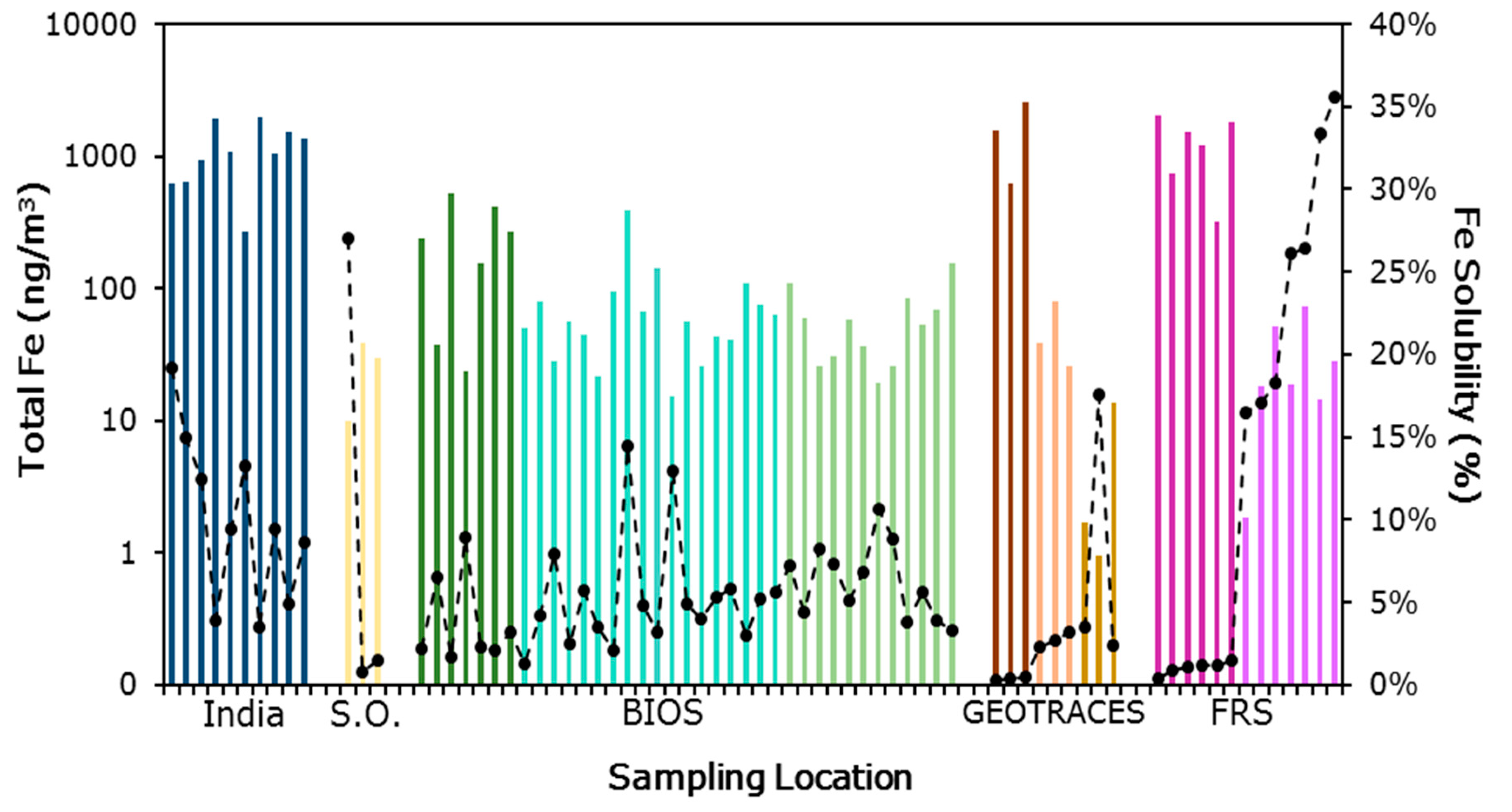
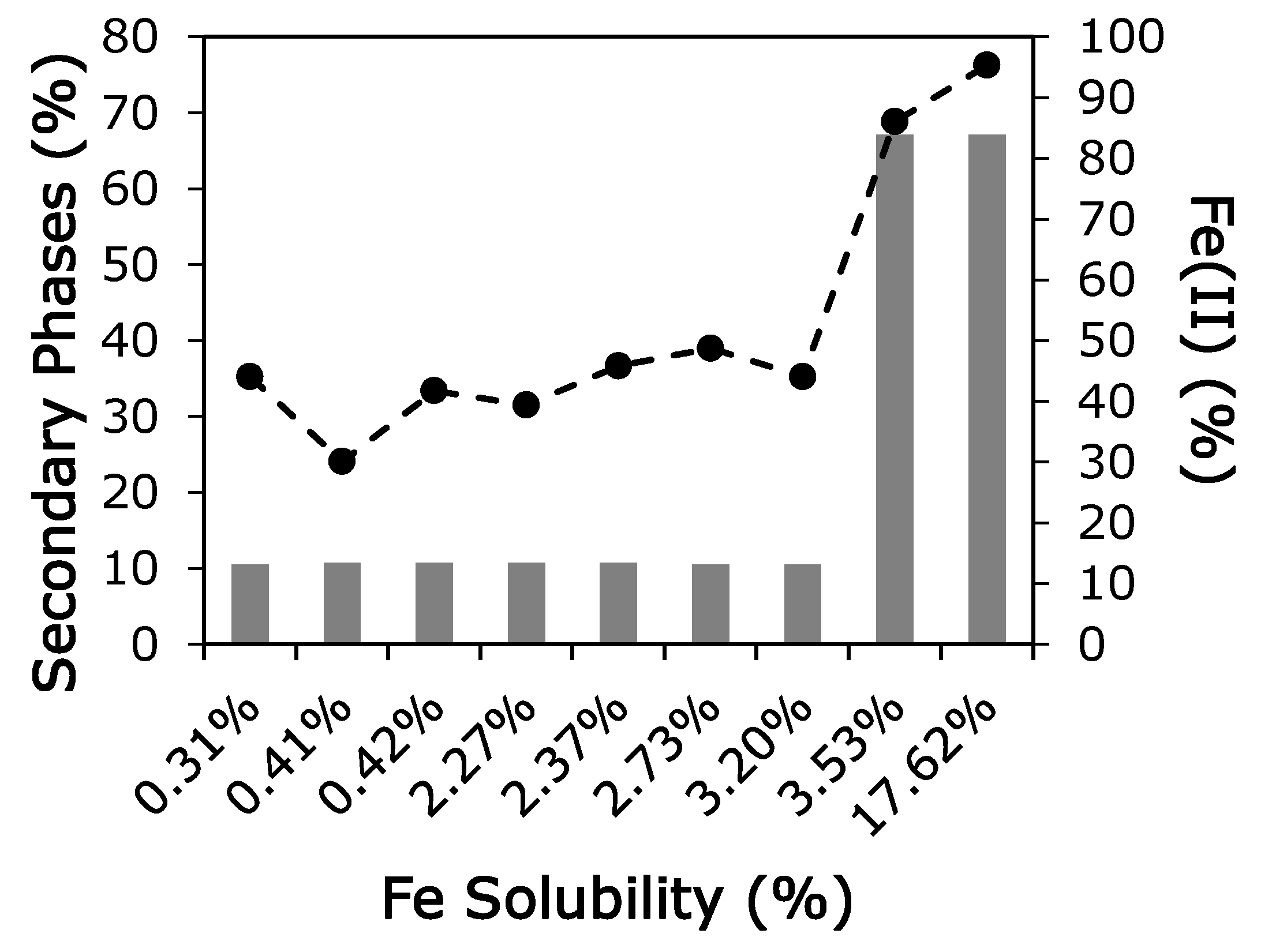
3.1. Iron Solubility

The total solubility of iron varied widely across the five different sampling locations (Tables S4 and S5). The highest soluble iron concentrations were found in samples from India, which contained 90 ± 26 ng/m3 of soluble iron on average (Figure 2). North African influenced samples from Finokalia Research Station exhibited the second highest levels of soluble iron (averaging 32 ± 52 ng/m3) and contain on average four times more soluble iron than the European influenced samples (7.4 ± 6.3 ng/m3) collected at the same sampling location. Similar to Finokalia Research Station, North African influenced samples from the GEOTRACES cruise contained the highest levels of soluble iron (on average 6.0 ± 4.1 ng/m3). Samples with primarily marine influences—the GEOTRACES and Southern Ocean samples—averaged 0.18 ± 0.13 ng/m3 and 1.2 ± 1.4 ng/m3 of soluble iron, respectively. North-American-influenced samples from the GEOTRACES collection averaged the same magnitude of soluble iron (1.3 ± 0.78 ng/m3) as the year-long collection of BIOS samples (3.8 ± 7.9 ng/m3).
However, when the fractional solubility of iron was considered (percentage of the total iron that is water solubilized) in lieu of total solubility, trends begin to emerge. European influenced samples from Finokalia Research Station had the most fractional soluble iron, followed by samples dominated by marine influences. In the samples for which North African mineral dust was mixed with anthropogenically influenced North American air masses, such as at the Bermuda site, aerosol iron often had a higher fractional iron solubility than samples that contained a stronger North African mineral dust influence (Figure 2). Fractional iron solubility in the Indian samples is also high, generally >5%, possibly indicating anthropogenic contributions of soluble iron.

3.2. Oxidation State

Samples from India contained primarily Fe(III), with only one bulk sample showing an Fe(II) signal of 2.1% (reflecting that 2.1% of the Fe in the sample is in this oxidation state) (Tables S4 and S5). This was similar to the findings for Southern Ocean samples, where two of the three samples contained only Fe(III), and the final sample contained about 90% Fe(III). At Finokalia Research Station, samples with a European influence tended to contain more reduced iron (13.5% on average) than samples with a North African influence (3.5% on average). In contrast, GEOTRACES samples contained at least 30% Fe(II) at the bulk level and could be dominated by Fe(II) (>95%). BIOS samples all contained at least 30% Fe(II) with Fe(II) reaching levels of about 75% in some bulk samples. Fe(II) is generally considered more soluble than Fe(III), but this relationship was not seen in our data [43]. When all the data was considered, there was a wide range of fractional iron solubility at each oxidation state, as represented by the position of the pre-edge centroid (Figure S1), indicating the absence of a direct relationship between iron oxidation state and the fractional solubility of aerosol iron.

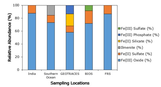
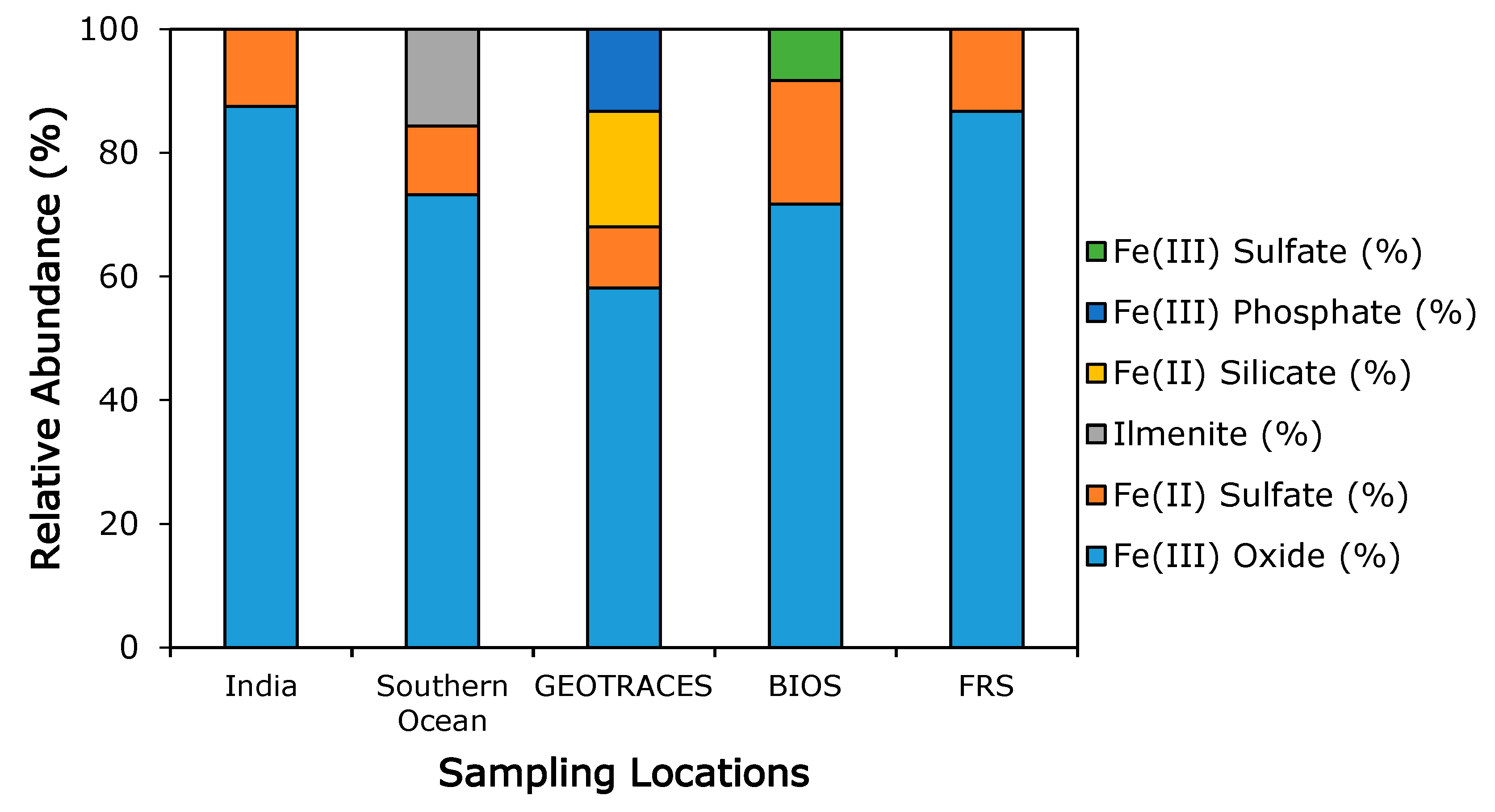
3.3. Iron Mineralogy

At the bulk level, nearly all the samples were dominated by Fe(III) oxides. The dominance of Fe(III) oxides in samples regardless of source region was surprising. This may reflect derivation of aerosols from highly weathered materials at the uppermost levels of land surfaces that tend to be rich in iron oxides. Fe(II) sulfates were present in most samples across all locations (Figure 3 and Tables S6 and S7). At both Finokalia Research Station and in India, the mineralogy was consistent across all bulk samples. Finokalia Research Station contained a combination of Fe(III) oxides (86.7 ± 0.5%) and Fe(II) sulfates (13.3 ± 0.5%). Indian samples also contained Fe(III) oxides (87.5 ± 2.1%) and Fe(II) sulfates (12.5 ± 1.5%). BIOS samples were generally consistent in composition containing Fe(III) oxides (81.3 ± 2%) and Fe(II) sulfates (18.7 ± 1%); however, five samples contained a combination of Fe(II) sulfates (38.5 ± 0.4%) and Fe(III) sulfates (61.5 ± 20.8%). Samples from the Southern Ocean belonged to one of two compositional groups. One group contained Fe(III) oxides (83.3 ± 9.4%) and Fe(II) sulfates (16.7 ± 0.7%), and the other group contained Fe(III) oxides (53.0 ± 1.9%) and ilmenite (47.0 ± 4%). GEOTRACES samples contained three compositional groups at the bulk level. Samples contained either a combination of: Fe(III) oxides (32.9 ± 10.3%), Fe(II) sulfates (28.7 ± 13.9%), and Fe(III) phosphates (38.4 ± 9.0%); Fe(III) oxides (89.5 ± 0%) and Fe(II) sulfates (10.5 ± 4%); or Fe(III) oxides (47.2 ± 12.1%), Fe(III) phosphates (10.7 ± 11.1%), and Fe(II) silicates (42.1 ± 11%).
A total of 157 individual particles were examined for iron mineralogy across the five different sample sets. Individual particles were generally more diverse in mineralogy than the bulk mineralogy (Table S7). Individual particles sampled from India belong to three mineralogical groups and were either dominated by Fe(III) oxides or Fe(II) silicates. Individual particles sampled from the Southern Ocean contained a combination of Fe(III) oxides and Fe(II) sulfates or were dominated by Fe(III) phosphates. Individual particles from Finokalia Research Station contained largely iron oxides. Some particles also contained minor quantities of ilmenite, an iron oxide containing titanium. Individual particles sampled from Finokalia Research Station also contained ilmenite but were largely dominated by Fe(III) oxides. Individual particles from Bermuda were largely a mixture of Fe(III) oxides and Fe(II) silicates. Individual particles sampled from the GEOTRACES transect had a strong presence of Fe(II and III) sulfates and Fe(III) phosphates with only minor contributions from Fe(III) oxides. The general dominance of iron oxides and sulfates was also seen in these individual particle analyses. In general, the phases identified in individual particles were consistent with the ones observed in bulk samples. In contrast to bulk spectra, which often have contributions from several different iron minerals, individual particle spectra were typically easier to fit with Athena [61]. Identification of phases in the individual particles supports their choice when modeling bulk spectra. Bulk spectra should be viewed as more representative of the overall iron mineralogy of a sample because they access particles across the entire spectrum of size ranges present in a sample.

4. Discussion

There are several hypothesized controlling factors for aerosol iron solubility, including composition and mineralogy, oxidation state, cloud processing, acidic reactions, organic ligand dissociation, and photoreduction [13,16,18,65,66,67,68]. In ambient aerosol samples, finding direct evidence of these mechanisms is challenging. Here, we focus primarily on the roles of composition, acidic reactions, oxidation state, and by extension photoreduction, which may influence the solubility of aerosol iron. Photoreduction pathways have been shown to play a key role in iron transformation in laboratory based experiments [69,70]; however, nitric acid suppresses the fraction of dissolved Fe(II) at low pH [26]. This suggests that these particle aging mechanisms further confounds the identification of a particular mechanism in ambient aerosol samples.
When data from India, the Southern Ocean, Bermuda, GEOTRACES, and Finokalia Research Station were considered together, there were no clear relationships between traditional factors that are typically associated with iron solubility. Composition (as a function of total iron content, R2 = 0.027) and oxidation state of iron (R2 = 0.058) are both not correlated with the fractional solubility of iron, suggesting that solubility of iron may not be linked to a specific iron phase or oxidation state (Figure S1). This is in contrast to evidence suggesting that photoreduction of iron occurs during the long-range transport of marine aerosol [43,65]. While our samples cover a wide range of transport distances, and presumably transport times, the absence of a direct relationship between iron solubility and oxidation state may stem from insufficient transport times for a large portion of our sample library, as detailed in Table S2. Photoreduction mechanisms working to solubilize mineral dust have been suggested to need more than 10 days of transport to show significant solubilization effects [71]. Composition can also dictate how photochemical mechanisms will proceed. Even within a general class of minerals, such as Fe(III) oxides, various minerals have variable levels of susceptibility to photochemical processing [35].
Correlation seen between inorganic acids, sulfuric acid, and nitric acid, and the solubility of aerosol iron had been used as evidence for acidic reactions promoting the solubility of iron in mineral dust [47,72,73]. Here, there was no relationship between total inorganic acidity (sum of sulfuric and nitric acids) (R2 = 0.0016), nitrate (R2 = 7 × 10⁻⁶), or non-sea-salt sulfate (R2 = 0.17) and the fractional solubility of iron. However, when pH was modelled with ISORROPIA [56,57], a trend indicates one possible explanation (Figure 4). When the pH is approximately neutral, a range from approximately 4 to 8, the solubility of iron is relatively low, but as the pH drops below 4, the fractional solubility of iron rapidly increases, up to nearly 35%. This behavior is consistent with the speciation of Fe(III), determined using the standard selection in the Mineql+ database to create an Fe(III) speciation diagram [74], where below a pH of approximately 3, the abundance of dissolved Fe(III) sharply increases [75,76,77]. This suggests that dissolved Fe(III) production is a consequence of acidic reactions in the atmosphere as would be expected for acidic species acting on a largely Fe(III) oxide composition. So only in the acidic range, when sufficient acidic species have aggregated on a particle, can the protons act to solubilize iron.
The mineralogy of aerosol iron is also key to understanding the acidic reactions that are likely at work. Heterogeneous mineralogy of aerosol iron can lead to iron with different levels of susceptibility to acid mobilization that act at different time scales [28,30,78]. Acidification of mineral dust has shown that iron will first undergo rapid iron dissolution, followed by a continued iron release at a much slower rate [78]. These differences in the rate of iron dissolution were linked to mineralogy, where the rapidly solubilizing iron is likely ferrihydrite, an amorphous iron oxide. The iron phases that undergo slow dissolution under acidic conditions are likely crystalline iron oxide phases and clay minerals [78]. Generally, amorphous iron oxides, like ferrihydrite, account for only 2% of aerosol iron, while more crystalline iron minerals and clays can account for up to 40% of the total aerosol iron [78]. The dominance of Fe(III) oxides in our aerosols (Figure 3), is consistent with the observed low to medium levels of fractional iron solubility.
Alteration of clay mineral phases to produce soluble iron minerals, such as ferrihydrite, has been shown to occur as a result of chemical reactions during atmospheric transport [79]. Traditional indicators of aerosol acidity, such as pH, suggest that acidic reactions are likely solubilizing iron, and our observations of iron phosphates and Fe(II and III) sulfates provide further support that acidic reactions are occurring. Although iron phosphates and sulfates may be found locally at emission sources, they do not typically occur in natural environments at high concentrations. To account for the concentrations of these phases seen in aerosol samples across all sampling locations, secondary atmospheric processes are likely at work. Iron phosphates and sulfates may form as a result of acidic processes that solubilize iron and phosphorus minerals through reactions with sulfuric and nitric acid species. One likely source of phosphorus mobilized under acidic conditions is the mineral apatite which has been identified as a common constituent in aerosols [80]. Such acidic processes can create an aqueous solution rich in dissolved iron, phosphorus, and sulfur which favor the precipitation of secondary mineral phases [23]. However, acids can be buffered by reactions associated with carbonate minerals commonly found in mineral dust [66,81]. Furthermore, aerosol pH undergoes diel fluctuations [82] that will cause the process of acidic transformation to be intermittent and slow. Three to five days are necessary to solubilize 1–2% of iron under similar acidic conditions of a deliquescent mineral dust particle [66,83]. Varying levels of reactive carbonate minerals in dust combined with the time-dependent impact of diel fluctuations on pH would lead to the observed variations in the concentrations of secondary phosphates, sulfates, and Fe(III) oxides in particles.
Aerosol source region may also influence the solubility of iron [84,85]. In this study, three sampling locations received air masses from different source regions: Finokalia Research Station, BIOS, and the GEOTRACES transect. At Finokalia Research Station, two distinct air masses were collected—anthropogenically influenced European air masses and mineral-dust laden North African air masses. North African air masses exhibit low fractional iron solubility and high pH, while samples from European air masses have higher fractional solubility and lower pH, possibly due to the anthropogenic contributions of nitrates and sulfates, affecting pH in these air masses [84,85]. At the Bermuda location, no correlations between aerosol iron solubility and source region, North African vs. North American, were present. However, the effects of source region on aerosol iron solubility could be subtly seen, where the average solubility of iron from North American air masses (6.3 ± 2.3%) was 1.5 times higher than the average iron solubility of North African air masses (3.8 ± 2.8%). Higher solubility in anthropogenically influenced aerosols may in part be influenced by their co-emission with acidic gases or their higher solubility at emission, in the case of biomass burning [31,73,85,86,87]. Samples collected on the GEOTRACES cruise also showed trends in iron solubility that were not apparent in the larger dataset. The composition (R2 = 0.53) and oxidation state (R2 = 0.64) were correlated with iron solubility (Figure 5). The higher levels of Fe(II) present in marine aerosol samples corresponded to increased iron solubility, which could be evidence of a reductive process, such as photoreduction. Moreover, these marine samples also had the highest quantities of Fe(II and III) sulfates and Fe(III) phosphates, phases that can be formed as a result of secondary processes that occur in the atmosphere.
Studies of mineral dust have also suggested a physical control over the solubility of aerosol iron, where larger particles are removed during atmospheric transport [88]. Compositional differences or changes in surface area to volume ratio in different particle size classes could have a potentially strong influence iron solubility [88,89]. Differences in sample collection techniques for the sample sets from different regions in this study resulted in differences in the size fractions collected. However, no clear trends in solubility emerged when comparing samples of different size fractions in our data set [88]. Another potential control of aerosol iron solubility is the presence of ligands that are thought to stabilize Fe(II) in solution and can also participate in ligand mediated photochemical reactions [90,91]. These physical processes along with ligand promoted iron dissolution are mechanisms that were not evaluated in this study. Variations in the impact of these physical and chemical processes in ambient aerosol could help explain the lack of direct overall correspondence between aerosol iron solubility, composition, and oxidation state in the global dataset.

5. Conclusions

This study presents an analysis of aerosol soluble iron characteristics from five different locations, on both a bulk-mass and individual-particle basis. In general, the total and soluble-iron trends seen in this data compilation are similar to those seen in other aerosol iron data sets for specific regions [33,34,47,73,89,92,93]. For aerosol iron, samples that are high in total iron have low fractional iron solubility, and samples with low total iron have higher fractional iron solubility [86]. This could reflect the influence of aerosol source region, where aerosols with high total iron tend to come from mineral dust sources, which can have significant buffer capacity. This contrasts with aerosols from anthropogenically influenced air masses that generally have lower buffer capacity and more acidic species or contribution from combustion sources with high iron solubility [94].
In the natural environment, the various chemical transformations of aerosols occurring during atmospheric transport may not only occur on different time scales, but the mechanisms can also have complex interactions with each other. For example, one study noted marine samples to be 5–17 times more soluble than samples containing significant anthropogenic influence when acidified to the same pH, and this increased solubility was attributed to conversion of Fe(III) to Fe(II) via photoreduction [65]. While in our data, acidification appears to be a key mechanism that affects aerosol iron regardless of source region, the findings of Zhuang et al. [17] demonstrate that one factor alone cannot be considered to control the solubility of aerosol iron. The observed variations in composition, oxidation state, pH, and solubility of aerosol iron shown here suggest that chemical transformations occur during atmospheric transport of aerosols originating from diverse source regions. Acidification and source region appear to play a significant role in determining the solubility of aerosol iron, but these data also show that one universal rule of iron solubility should not be applied to estimate the solubility of aerosol iron on a global scale. Better quantification of iron speciation and better understanding of the evolution of iron solubility in aerosols is needed. This in turn emphasizes the need to conduct further studies on environmental samples, both in situ and under controlled conditions, to quantify physical processes and chemical transformations that happen to aerosols during atmospheric transport and their effects on iron solubility.

Supplementary Materials

The following are available online at https://www.mdpi.com/2073-4433/9/5/201/s1, Figure S1: Pre-edge Centroid vs Fe Solubility, Table S1: Sample collection information for India, Southern Ocean, Finokalia Research Station and GEOTRACES samples, Table S2: Sample collection information for samples collected at BIOS, Table S3: Sample Collection Locations, Table S4: BIOS Aerosol Data, Table S5: India, GEOTRACES, Southern Ocean and Finokalia Research Station Aerosol Data, Table S6: Correlation values for iron solubility, Table S7: Composition of bulk aerosol and individual aerosol particle samples

Author Contributions

E.D.I. and A.F.L. are responsible for the experiments and much of the content. E.D.I., A.F.L. and E.C. drafted the manuscript. Y.F. initiated the project and contributed resources. B.L. assisted while the team was at APS. Y.G., W.M.L., P.L.M., N.M., A.N., R.U.S., S.S. and K.V. provided samples and insights. All authors contributed to this manuscript.

Acknowledgments

This material is based upon work supported by the National Science Foundation under Grants OCE 1357375 (EDI), OCE 1658181 (EDI), OCE-0929919 (WML), OCE-1034764 (WML), OCE-1658311 (PLM), OPP-0944589 (YG) and PLR-1341494 (YG). The data used to produce these results is available upon request to the corresponding author. Any opinions, findings, and conclusions or recommendations expressed in this material are those of the authors and do not necessarily reflect the views of the National Science Foundation. Use of the Advanced Photon Source and support to YF and BL are provided by Argonne National Laboratory under the U.S. Department of Energy contract DE-AC02-06CH11357. A portion of this work was performed at the National High Magnetic Field Laboratory, which is supported by National Science Foundation Cooperative Agreement DMR-1157490 and the State of Florida. NM and KV acknowledge support from European Union (European Social Fund) and Greek national funds through the Operational Program “Education and Lifelong Learning” of the National Strategic Reference Framework Research Funding Program, ARISTEIA.

Conflicts of Interest

The authors declare no conflict of interest.

References

  1. Schulz, M.; Prospero, J.M.; Baker, A.R.; Dentener, F.J.; Ickes, L.; Liss, P.S.; Mahowald, N.M.; Nickovic, S.; Perez Garcia-Pando, C.; Rodrigeuz, S.; et al. Atmospheric transport and deposition of mineral dust to the ocean: Implications for research needs. Environ. Sci. Technol. 2012, 46, 10390–10404. [Google Scholar] [CrossRef] [PubMed]
  2. Boyd, P.W.; Mackie, D.S.; Hunter, K.A. Aerosol iron deposition to the surface ocean—Modes of iron supply and biological responses. Mar. Chem. 2010, 120, 128–143. [Google Scholar] [CrossRef]
  3. Martin, J.H. Glacial-interglacial CO2 change: The iron hypothesis. Paleoceanography 1990, 5, 1–13. [Google Scholar] [CrossRef]
  4. Li, W.; Xu, L.; Liu, X.; Zhang, J.; Lin, Y.; Yao, X.; Gao, H.; Zhang, D.; Chen, J.; Wang, W.; et al. Air pollution–aerosol interactions produce more bioavailable iron for ocean ecosystems. Sci. Adv. 2017, 3, e1601749. [Google Scholar] [CrossRef] [PubMed]
  5. Moore, C.M.; Mills, M.M.; Arrigo, K.R.; Berman-Frank, I.; Bopp, L.; Boyd, P.W.; Galbraith, R.; Geider, R.J.; Guieu, C.; Jaccard, S.L.; et al. Processes and patterns of oceanic nutrient limitation. Nat. Geosci. 2013, 6, 701–710. [Google Scholar] [CrossRef] [Green Version]
  6. De Jong, J.; Schoemann, V.; Lannuzel, D.; Croot, P.; de Baar, H.; Tison, J.-L. Natural iron fertilization of the Atlantic sector of the Southern Ocean by continental shelf sources of the Antarctic Peninsula. J. Geophys. Res. Biogeosci. 2012, 117. [Google Scholar] [CrossRef]
  7. Coale, K.H.; Johnson, K.S.; Chavez, F.P.; Buesseler, K.O.; Barber, R.T.; Brzezinski, M.A.; Cochlan, W.P.; Millero, F.J.; Falkowski, P.G.; Bauer, J.E.; et al. Southern Ocean iron enrichment experiment: Carbon cycling in high- and low-si waters. Science 2004, 304, 408–414. [Google Scholar] [CrossRef] [PubMed]
  8. Buesseler, K.O.; Andrews, J.E.; Pike, S.M.; Charette, M.A. The effects of iron fertilization on carbon sequestration in the Southern Ocean. Science 2004, 304, 414–417. [Google Scholar] [CrossRef] [PubMed]
  9. Boyd, P.W.; Watson, A.J.; Law, C.S.; Abraham, E.R.; Trull, T.; Murdoch, R.; Bakker, D.C.E.; Bowie, A.R.; Buesseler, K.O.; Chang, H.; et al. A mesoscale phytoplankton bloom in the polar Southern Ocean stimulated by iron fertilization. Nature 2000, 407, 695–702. [Google Scholar] [CrossRef] [PubMed]
  10. Coale, K.H.; Johnson, K.S.; Fitzwater, S.E. A massive phytoplankton bloom induced by an ecosystem-scale iron fertilization experiment in the equitorial Pacific Ocean. Nature 1996, 383, 495–501. [Google Scholar] [CrossRef] [PubMed]
  11. Mahowald, N.; Baker, A.R.; Bergametti, G.; Brooks, N.; Duce, R.A.; Jickells, T.D.; Kubilay, N.; Prospero, J.M.; Tegen, I. Atmospheric global dust cycle and iron inputs to the ocean. Glob. Biogeochem. Cycle 2005, 19. [Google Scholar] [CrossRef]
  12. Jickells, T.D.; An, Z.S.; Andersen, K.K.; Baker, A.R.; Bergametti, G.; Brooks, N.; Cao, J.J.; Boyd, P.W.; Duce, R.A.; Hunter, K.A.; et al. Global iron connections between desert dust, ocean biogeochemistry, and climate. Science 2005, 308, 67–71. [Google Scholar] [CrossRef] [PubMed]
  13. Ito, A.; Shi, Z. Delivery of anthropogenic bioavailable iron from mineral dust and combustion aerosols to the ocean. Atmos. Chem. Phys. 2016, 16, 85–99. [Google Scholar] [CrossRef] [Green Version]
  14. Spolaor, A.; Vallelonga, P.; Cozzi, F.; Gabrielli, P.; Varin, C.; Kehrwald, N.; Zennaro, P.; Boutron, C.F.; Barbante, C. Iron speciation in aerosol dust influences iron bioavailability over glacial-interglacial timescales. Geophys. Res. Lett. 2013, 40, 1618–1623. [Google Scholar] [CrossRef]
  15. Ito, T.; Nenes, A.; Johnson, M.S.; Meskhidze, N.; Deutsch, C. Acceleration of oxygen decline in the tropical pacific over the past decades by aerosol pollutants. Nat. Geosci. 2016, 9, 443–447. [Google Scholar] [CrossRef]
  16. Baker, A.R.; Croot, P.L. Atmospheric and marine controls on aerosol iron solubility in seawater. Mar. Chem. 2010, 120, 4–13. [Google Scholar] [CrossRef] [Green Version]
  17. Zhuang, G.; Yi, Z.; Duce, R.A.; Brown, P.R. Chemistry of iron in marine aerosols. Glob. Biogeochem. Cycle 1992, 6, 161–173. [Google Scholar] [CrossRef]
  18. Shi, Z.; Krom, M.D.; Jickells, T.D.; Bonneville, S.; Carslaw, K.S.; Mihalopoulos, N.; Baker, A.R.; Benning, L.G. Impacts on iron solubility in the mineral dust by processes in the source region and the atmosphere: A review. Aeolian Res. 2012, 5, 21–42. [Google Scholar] [CrossRef]
  19. Journet, E.; Desboeufs, K.V.; Caquineau, S.; Colin, J.L. Mineralogy as a critical factor of dust iron solubility. Geophys. Res. Lett. 2008, 35. [Google Scholar] [CrossRef]
  20. Zhu, X.; Prospero, J.M.; Savoie, D.L.; Millero, F.J.; Zika, R.G.; Saltzman, E.S. Photoreduction of iron(III) in marine mineral aerosol solutions. J. Geophys. Res. Atmos. 1993, 98, 9039–9046. [Google Scholar] [CrossRef]
  21. Witt, M.L.I.; Mather, T.A.; Baker, A.R.; De Hoog, J.C.M.; Pyle, D.M. Atmospheric trace metals over the south-west Indian Ocean: Total gaseous mercury, aerosol trace metal concentrations and lead isotope ratios. Mar. Chem. 2010, 121, 2–16. [Google Scholar] [CrossRef]
  22. Wiederhold, J.G.; Kraemer, S.M.; Teutsch, N.; Borer, P.M.; Halliday, A.N.; Kretzschmar, R. Iron isotope fractionation during proton-promoted, ligand-controlled, and reductive dissolution of goethite. Environ. Sci. Technol. 2006, 40, 3787–3793. [Google Scholar] [CrossRef] [PubMed]
  23. Nenes, A.; Krom, M.D.; Mihalopoulos, N.; Van Cappellen, P.; Shi, Z.; Bougiatioti, A.; Zarmpas, P.; Herut, B. Atmospheric acidification of mineral aerosols: A source of bioavailable phosphorus for the oceans. Atmos. Chem. Phys. 2011, 11, 6265–6272. [Google Scholar] [CrossRef]
  24. Shi, Z.; Krom, M.D.; Bonneville, S.; Benning, L.G. Atmospheric processing outside clouds increases soluble iron in mineral dust. Environ. Sci. Technol. 2015, 49, 1472–1477. [Google Scholar] [CrossRef] [PubMed]
  25. Shi, Z.; Krom, M.D.; Bonneville, S.; Baker, A.R.; Jickells, T.D.; Benning, L.G. Formation of iron nanoparticles and increase in iron reactivity in mineral dust during simulated cloud processing. Environ. Sci. Technol. 2009, 43, 6592–6596. [Google Scholar] [CrossRef] [PubMed]
  26. Cwiertny, D.M.; Baltrusaitis, J.; Hunter, G.J.; Laskin, A.; Scherer, M.M.; Grassian, V.H. Characterization and acid-mobilization study of iron-containing mineral dust source materials. J. Geophys. Res. 2008, 113. [Google Scholar] [CrossRef]
  27. Weber, R.J.; Guo, H.; Russell, A.G.; Nenes, A. High aerosol acidity despite declining atmospheric sulfate concentrations over the past 15 years. Nat. Geosci. 2016, 9, 282–285. [Google Scholar] [CrossRef]
  28. Ito, A.; Feng, Y. Role of dust alkalinity in acid mobilizaiton of iron. Atmos. Chem. Phys. 2010, 10, 9237–9250. [Google Scholar] [CrossRef] [Green Version]
  29. Hennigan, C.J.; Izumi, J.; Sullivan, A.P.; Weber, R.J.; Nenes, A. A critical evaluation of proxy methods used to estimate the acidity of atmospheric particles. Atmos. Chem. Phys. 2015, 15, 2775–2790. [Google Scholar] [CrossRef]
  30. Sullivan, R.C.; Guazzotti, S.A.; Sodeman, D.A.; Prather, K.A. Direct observations of the atmospheric processing of Asian mineral dust. Atmos. Chem. Phys. 2007, 7, 1213–1236. [Google Scholar] [CrossRef]
  31. Oakes, M.; Ingall, E.D.; Lai, B.; Shafer, M.M.; Hays, M.D.; Liu, Z.G.; Russell, A.G.; Weber, R.J. Iron solubility related to particle sulfur content in source emission and ambient fine particles. Environ. Sci. Technol. 2012, 46, 6637–6644. [Google Scholar] [CrossRef] [PubMed]
  32. Hoffmann, P.; Dedik, A.N.; Ensling, J.; Weinbruch, S.; Weber, S.; Sinner, T.; Gutlich, P.; Ortner, H.M. Speciation of iron in atmospheric aerosol samples. J. Aerosol Sci. 1996, 27, 325–337. [Google Scholar] [CrossRef]
  33. Buck, C.S.; Landing, W.M.; Resing, J.A.; Lebon, G.T. Aerosol iron and aluminum solubility in the northwest Pacific Ocean: Results from the 2002 IOC cruise. Geochem. Geophys. Geosyst. 2006, 7. [Google Scholar] [CrossRef]
  34. Gao, Y.; Xu, G.; Zhan, J.; Zhang, J.; Li, W.; Lin, Q.; Chen, L.; Lin, H. Spatial and particle size distributions of atmospheric dissolvable iron in aerosols and its input to the Southern Ocean and coastal East Antarctica. J. Geophys. Res. Atmos. 2013, 118, 634–648. [Google Scholar] [CrossRef]
  35. Cornell, R.M.; Schindler, P.W. Photochemical dissolution of goethite in acid/oxalate solution. Clays Clay Miner. 1987, 35, 347–352. [Google Scholar] [CrossRef]
  36. Xu, N.; Gao, Y. Characterization of hematite dissolution affected by oxalate coating, kinetics and pH. Appl. Geochem. 2008, 23, 783–793. [Google Scholar] [CrossRef]
  37. Cornell, R.M.; Schwertmann, U. The Iron Oxides, Structure, Properties, Reactions, Occurence and Uses; John Wiley: Hokoken, NJ, USA, 1996. [Google Scholar]
  38. Winton, V.H.L.; Bowie, A.R.; Edwards, R.; Keywood, M.; Townsend, A.T.; van der Merwe, P.; Bollhofer, A. Fractional iron solubility of atmospheric iron inputs to the Southern Ocean. Mar. Chem. 2015, 177, 20–32. [Google Scholar] [CrossRef]
  39. Majestic, B.J.; Schauer, J.J.; Shafer, M.M. Application of synchrotron radiation for measurement of iron red-ox speciation in atmospherically processed aerosols. Atmos. Chem. Phys. 2007, 7, 2475–2487. [Google Scholar] [CrossRef]
  40. Fittschen, U.E.A.; Meirer, F.; Streli, C.; Wobrauschek, P.; Thiele, J.; Falkenberg, G.; Pepponi, G. Characterization of atmospheric aerosols using synchroton radiation total reflection X-ray fluorescence and Fe K-edge total reflection X-ray fluorescence-X-ray absorption near-edge structure. Spectrochim. Acta Part B At. Spectrosc. 2008, 63, 1489–1495. [Google Scholar] [CrossRef]
  41. Dabek-Zlotorzynska, E.; Kelly, M.; Chen, H.; Chakrabarti, C.L. Evaluation of capillary electrophoresis combined with a BCR sequential extraction for determining distribution of Fe, Zn, Cu, Mn, and Cd in airborne particulate matter. Anal. Chim. Acta 2003, 498, 175–187. [Google Scholar] [CrossRef]
  42. Johnson, M.S.; Meskhidze, N. Atmospheric dissolved iron deposition to the global oceans: Effects of oxalate-promoted dissolution, photochemical redox cycling, and dust mineralogy. Geosci. Model Dev. Discuss. 2013, 6, 1137–1155. [Google Scholar] [CrossRef]
  43. Longo, A.F.; Feng, Y.; Lai, B.; Landing, W.M.; Shelley, R.U.; Nenes, A.; Mihalopoulos, N.; Violaki, K.; Ingall, E.D. Influence of atmospheric processes on the solubility and composition of iron in saharan dust. Environ. Sci. Technol. 2016, 50, 6912–6920. [Google Scholar] [CrossRef] [PubMed]
  44. Oakes, M.; Weber, R.J.; Lai, B.; Russell, A.; Ingall, E.D. Characterization of iron speciation in urban and rural single particles using xanes spectroscopy and micro X-ray fluorescence measurements: Investigating the relationship between speciation and fractional iron solubility. Atmos. Chem. Phys. 2012, 12, 745–756. [Google Scholar] [CrossRef] [Green Version]
  45. Moffet, R.C.; Furutani, H.; Rodel, T.C.; Henn, T.R.; Sprau, P.O.; Laskin, A.; Uematsu, M.; Gilles, M.K. Iron speciation and mixing in single aerosol particles from Asian continental outflows. J. Geophys. Res. 2012, 117. [Google Scholar] [CrossRef]
  46. Weber, S.; Hoffmann, P.; Ensling, J.; Dedik, A.N.; Weinbruch, S.; Miehe, G.; Gutlich, P.; Ortner, H.M. Characterization of iron compounds from urban and rural aerosol sources. J. Aerosol Sci. 2000, 31, 987–997. [Google Scholar] [CrossRef]
  47. Srinivas, B.; Sarin, M.; Rengarajan, R. Atmospheric transport of mineral dust from the indo-gangeticplain: Temporal variability, acid processing, and iron solubility. Geochem. Geophys. Geosyst. 2014, 15, 3226–3243. [Google Scholar] [CrossRef]
  48. Markaki, Z.; Oikonomou, K.; Kocak, M.; Kouvarakis, G.; Chaniotaki, A.; Kubilay, N.; Mihalopoulos, N. Atmospheric deposition of inorganic phosphorus in the Levantine Basin, eastern Mediterranean: Spatial and temporal variability and its role in seawater productivity. Limnol. Oceanogr. 2003, 48, 1557–1568. [Google Scholar] [CrossRef]
  49. Shelley, R.U.; Morton, P.L.; Landing, W.M. Elemental ratios and enrichment factors in aerosols from the US-GEOTRACES North Atlantic transects. Deep Sea Res. Part I Trop. Stud. Oceanogr. 2015, 116, 262–272. [Google Scholar] [CrossRef]
  50. Stein, A.F.; Draxler, R.R.; Rolph, G.D.; Stunder, B.J.B.; Cohen, M.D.; Ngan, F. Noaa’s hysplit atmospheric transport and dispersion modeling system. Bull. Am. Meteorol. Soc. 2015, 96, 2059–2077. [Google Scholar] [CrossRef]
  51. Rolph, G.; Stein, A.; Stunder, B. Real-time environmental applications and display system: Ready. Environ. Model. Softw. 2017, 95, 210–228. [Google Scholar] [CrossRef]
  52. Stookey, L.L. Ferrozine—A new spectrophotometric reagent for iron. Anal. Chem. 1970, 42, 779–781. [Google Scholar] [CrossRef]
  53. Kadko, D.; Landing, W.M.; Shelley, R.U. A novel tracer technique to quantify the atmospheric flux of trace elements to remote ocean regions. J. Geophys. Res. Oceans 2015, 119, 848–858. [Google Scholar] [CrossRef]
  54. Morton, P.L.; Landing, W.M.; Hsu, S.C.; Milne, A.; Aguilar-Islas, A.M.; Baker, A.R.; Bowie, A.R.; Buck, C.S.; Gao, Y.; Gichuki, S.; et al. Methods for the sampling and analysis of marine aerosols: Results from the 2008 geotraces aerosol intercalibration experiment. Limnol. Oceanogr. 2013, 11, 62–78. [Google Scholar] [CrossRef] [Green Version]
  55. Bardouki, H.; Liakakou, H.; Economou, C.; Sciare, J.; Smolik, J.; Zdimal, V.; Eleftheriadis, K.; Ladaridis, M.; Dye, C.; Mihalopoulos, N. Chemical composition of size-resolved atmospheric aerosols in the eastern Mediterranean during summer and winter. Atmos. Environ. 2003, 37, 195–208. [Google Scholar] [CrossRef]
  56. Fountoukis, C.; Nenes, A. Isorropia II: A computationally efficient thermodynamic equilibrium model for K+–Ca2+–Mg2+–NH4+–Na+–SO42–NO3–Cl–H2O aerosols. Atmos. Chem. Phys. 2007, 7, 4639–4659. [Google Scholar] [CrossRef]
  57. Nenes, A.; Pandis, S.N.; Pilinis, C. Isorropia: A new thermodynamic equilibrium model for multiphase multicomponent inorganic aerosols. Aquat. Geochem. 1998, 4, 123–152. [Google Scholar] [CrossRef]
  58. Ingall, E.; Brandes, J.; Diaz, J.; de Jonge, M.; Paterson, D.; McNulty, I.; Elliott, W.; Northrup, P. Phosphorus k-edge xanes spectroscopy of mineral standards. J. Synchrotron Radiat. 2011, 18, 189–197. [Google Scholar] [CrossRef] [PubMed]
  59. Wilke, M.; Farges, F.; Petit, P.E.; Brown, G.E.; Martin, F. Oxidation state and coordination of fe in minerals: An fek-xanes spectroscopic study. Am. Mineral. 2001, 86, 714–730. [Google Scholar] [CrossRef]
  60. Bajt, S.; Sutton, S.R.; Delaney, J.S. X-ray microprobe analysis of iron oxidation-states in silicates and oxides using X-ray absorption near-edge structure (XANES). Geochim. Cosmochim. Acta 1994, 58, 5209–5214. [Google Scholar] [CrossRef]
  61. Ravel, B.; Newville, M. Athena, artemis, hephaestus: Data analysis for X-ray absorption spectroscopy using ifeffit. J. Synchrotron Radiat. 2005, 12, 537–541. [Google Scholar] [CrossRef] [PubMed]
  62. Marcus, M.A.; Lam, P.J. Visualising fe speciation diversity in ocean particulate samples by micro X-ray absorption near-edge spectroscopy. Environm. Chem. 2014, 11, 10–17. [Google Scholar] [CrossRef]
  63. Ingall, E.; Diaz, J.; Longo, A.; Oakes, M.; Finney, L.; Vogt, S.; Lai, B.; Yager, P.L.; Twining, B.S.; Brandes, J. Role of biogenic silica in the removal of iron from antarctic seas. Nat. Commun. 2013, 4, 1981. [Google Scholar] [CrossRef] [PubMed]
  64. Hesterberg, D. Chapter 11—Macroscale chemical properties and X-ray absorption spectroscopy of soil phosphorus. In Developments in Soil Science; Balwant, S., Markus, G., Eds.; Elsevier: New York City, NY, USA, 2010; Volume 34, pp. 313–356. [Google Scholar]
  65. Zhuang, G.; Yi, Z.; Duce, R.A.; Brown, P.R. Link between iron and sulphur cycles suggested by detection of Fe(n) in remote marine aerosols. Nature 1992, 335, 537–539. [Google Scholar] [CrossRef]
  66. Meskhidze, N.; Chameides, W.L.; Nenes, A.; Chen, G. Iron mobilization in mineral dust: Can anthropogenic SO2 emissions affect ocean productivity? Geophys. Res. Lett. 2003, 30. [Google Scholar] [CrossRef]
  67. Meskhidze, N.; Nenes, A.; Conant, W.C.; Seinfeld, J.H. Evaluation of a new cloud droplet activation parameterization with in situ data from CRYSTAL-FACE and CSTRIPE. J. Geophys. Res. Atmos. 2005, 110. [Google Scholar] [CrossRef]
  68. Hettiarachchi, E.; Hurab, O.; Rubasinghege, G. Atmospheric processing and iron mobilization of ilmenite: Iron-containing ternary oxide in mineral dust aerosol. J. Phys. Chem. A 2018, 122, 1291–1302. [Google Scholar] [CrossRef] [PubMed]
  69. Siefert, R.L.; Webb, S.M.; Hoffmann, M.R. Determination of photochemically available iron in ambient aerosols. J. Geophys. Res. 1996, 10, 14441–14449. [Google Scholar] [CrossRef]
  70. Siefert, R.L.; Pehkonen, S.O.; Erel, Y.; Hoffmann, M.R. Iron photochemistry of aqueous suspensions of ambient aerosol with added organic acids. Geochim. Cosmochim. Acta 1994, 58, 3217–3279. [Google Scholar] [CrossRef]
  71. Baker, A.R.; French, M.; Linge, K.L. Trends in aerosol nutrient solubility along a west-east transect of the saharan dust plume. Geophys. Res. Lett. 2006, 33. [Google Scholar] [CrossRef]
  72. Srinivas, B.; Sarin, M.M.; Kumar, A.K. Impact of anthropogenic sources on aerosol iron solubility over the Bay of Bengal and the Arabian Sea. Biogeochemistry 2012, 110, 257–268. [Google Scholar] [CrossRef]
  73. Kumar, A.; Sarin, M.; Srinivas, B. Aerosol iron solubility over bay of bengal: Role of anthropogenic sources and chemical processing. Mar. Chem. 2010, 121, 167–175. [Google Scholar] [CrossRef]
  74. Katsoyiannis, I.A.; Zouboulis, A.I. Removal of arsenic from contaminated water sources by sorption onto iron-oxide-coated polymeric materials. Water Res. 2002, 26, 5141–5155. [Google Scholar] [CrossRef]
  75. Wantala, K.; Sthiannopkao, S.; Srinameb, B.O.; Grisdanurak, N.; Kim, K.W.; Han, S. Arsenic adsorption by fe loaded on rh-mcm-41 synthesized from rice husk silica. J. Environ. Eng. ASCE 2012, 138, 119–128. [Google Scholar] [CrossRef]
  76. Sanchiz, J.; Esparza, P.; Dominguez, S.; Brito, F.; Mederos, A. Solution studies of complexes of iron(III) with iminodiacetic, alkyl-substituted iminodiacetic and nitrilotriacetic acids by potentiometry and cyclic voltammetry. Inorg. Chim. Acta 1999, 291, 158–165. [Google Scholar] [CrossRef]
  77. Salgado, P.; Melin, V.; Contreras, D.; Moreno, Y.; Mansilla, H.D. Fenton reaction driven by iron ligands. J. Chil. Chem. Soc. 2013, 58, 2096–2101. [Google Scholar] [CrossRef]
  78. Shi, Z.; Bonneville, S.; Krom, M.D.; Carslaw, K.S.; Jickells, T.D.; Baker, A.R.; Benning, L.G. Iron dissolution kinetics of mineral dust at low pH during simulated atmospheric processing. Atmos. Chem. Phys. 2011, 11, 995–1007. [Google Scholar] [CrossRef] [Green Version]
  79. Takahashi, Y.; Higashi, M.; Furukawa, T.; Mitsunobu, S. Change of iron species and iron solubility in Asian dust during the long-range transport from western China to Japan. Atmos. Chem. Phys. 2011, 11, 11237–11252. [Google Scholar] [CrossRef] [Green Version]
  80. Longo, A.F.; Ingall, E.D.; Diaz, J.M.; Oakes, M.; King, L.E.; Nenes, A.; Mihalopoulos, N.; Violaki, K.; Avila, A.; Benitez-Nelson, C.R.; et al. P-NEXFS analysis of aerosol phosphorus delivered to the Mediterranean Sea. Geophys. Res. Lett. 2014, 41, 4043–4049. [Google Scholar] [CrossRef]
  81. Ito, A.; Feng, Y. Iron mobilization in North African Dust. Procedia Environ. Sci. 2011, 6, 27–34. [Google Scholar] [CrossRef]
  82. Nikolauo, P.; Bougiatioti, A.; Stavroulas, I.; Kouvarakis, G.; Nenes, A.; Weber, R.J.; Kanakidou, M.; Mihalopoulos, N. Particle water and pH in the eastern Mediterranean: Sources variability and implications for nutrients availability. Atmos. Chem. Phys. 2016, 16, 4579–4591. [Google Scholar] [CrossRef]
  83. Guo, H.; Xu, L.; Bougiatioti, A.; Cerully, K.M.; Capps, S.L.; Hite, J.R.; Carlton, A.G.; Lee, S.-H.; Bergin, M.H.; Ng, N.L.; et al. Fine-particulate water and pH in the southeastern united states. Atmos. Chem. Phys. 2015, 15, 5211–5228. [Google Scholar] [CrossRef]
  84. Sholkovitz, E.R.; Sedwick, P.N.; Church, T.M. Influence of anthropogenic combustion emissions on the deposition of soluble aerosol iron to the ocean: Empirical estimates for island sites in the North Atlantic. Geochim. Cosmochim. Acta 2009, 73, 3981–4003. [Google Scholar] [CrossRef]
  85. Sedwick, P.; Sholkovitz, E.R.; Church, T.M. Impact of anthropogenic combustion emissions on the fractional solubility of aerosol iron: Evidence from the Sargasso Sea. Geochem. Geophys. Geosyst. 2007, 8. [Google Scholar] [CrossRef]
  86. Sholkovitz, E.R.; Sedwick, P.N.; Church, T.M.; Baker, A.R.; Powell, C.F. Fractional solubility of aerosol iron: Synthesis of a global-scale data set. Geochim. Cosmochim. Acta 2012, 89, 173–189. [Google Scholar] [CrossRef]
  87. Liu, W.; Wang, Y.; Russell, A.; Edgerton, E.S. Atmospheric aerosol over two urban–rural pairs in the southeastern United States: Chemical composition and possible sources. Atmos. Environ. 2005, 39, 4453–4470. [Google Scholar] [CrossRef]
  88. Baker, A.R.; Jickells, T.D. Mineral particle size as a control on aerosol iron solubility. Geophys. Res. Lett. 2006, 33. [Google Scholar] [CrossRef]
  89. Kumar, A.; Sarin, M. Aerosol iron solubility in a semi-arid region: Temporal trend and impact of anthropogenic sources. Tellus Ser. B Chem. Phys. Meteorol. 2009, 62, 125–132. [Google Scholar] [CrossRef]
  90. Wozniak, A.S.; Shelley, R.U.; Sleighter, R.L.; Abdulla, H.A.N.; Morton, P.L.; Landing, W.M.; Hatcher, P.G. Relationships among aerosol water soluble organic matter, iron and aluminum in European, North African, and Marine air masses from the 2010 US GEOTRACES cruise. Mar. Chem. 2013, 154, 24–33. [Google Scholar] [CrossRef]
  91. Paris, R.; Desboeufs, K.V.; Journet, E. Variability of dust iron solubility in atmospheric waters: Investigation of the role of oxalate organic complexation. Atmos. Environ. 2011, 45, 6510–6517. [Google Scholar] [CrossRef]
  92. Fu, H.B.; Shang, G.F.; Lin, J.; Hu, Y.J.; Hu, Q.Q.; Guo, L.; Zhang, Y.C.; Chen, J.M. Fractional iron solubility of aerosol particles enhanced by biomass burning and ship emissions in Shanghai, East China. Sci. Total Environ. 2014, 481, 377–391. [Google Scholar] [CrossRef] [PubMed]
  93. Takahashi, T.; Furukawa, T.; Kanai, Y.; Uematsu, M.; Zheng, G.; Marcus, M.A. Seasonal changes in Fe species and soluble Fe concentration in the atmosphere in the Northwest Pacific region based on the analysis of aerosols collected in Tsukuba, Japan. Atmos. Chem. Phys. 2013, 13, 7695–7710. [Google Scholar] [CrossRef]
  94. Luo, C.; Mahowald, N.M.; Meskhidze, N.; Chen, Y.; Siefert, R.L.; Baker, A.R.; Johansen, A.M. Estimation of iron solubility from observations and a global aerosol model. J. Geophys. Res. Atmos. 2005, 110. [Google Scholar] [CrossRef]
Figure 1. Global map with sampling locations indicated. Precise latitude and longitude for each sampling location can be found in Table S3.
Atmosphere 09 00201 g001
Figure 2. The total iron (colored bars, in ng/m3) and soluble iron (dashed black line, in %) are shown for each sample set, where each sample set and air mass source region are color coded as follows: India Atmosphere 09 00201 i001, Southern Ocean (S. O.) Atmosphere 09 00201 i002, BIOS Saharan air masses Atmosphere 09 00201 i003, BIOS mixed air masses Atmosphere 09 00201 i004, BIOS North American air masses Atmosphere 09 00201 i005, GEOTRACES Saharan air masses Atmosphere 09 00201 i006, GEOTRACES North American air masses Atmosphere 09 00201 i007, GEOTRACES marine air masses Atmosphere 09 00201 i008, Finokalia Research Station (FRS) Saharan air masses Atmosphere 09 00201 i009, and Finokalia Research Station European air masses Atmosphere 09 00201 i010. Generally, samples with the highest total iron have low fractional solubility of iron.
Atmosphere 09 00201 g002
Figure 3. Average aerosol iron mineralogy for each sample set is shown. Fe(III) oxides and Fe(II) sulfates are prevalent in all sample sets. GEOTRACES and BIOS samples also contain Fe(II) silicates, Fe(III) sulfates, and Fe(III) phosphates.
Atmosphere 09 00201 g003
Figure 4. The pH, modelled via ISORROPIA-II, for samples from the BIOS, GEOTRACES, and Finokalia Research Station sample sets shows that only when the pH is below approximately 4, or under acidic conditions, does the pH affect the fractional solubility of iron. The behavior of fractional solubility of aerosol iron as a function of pH is consistent with the speciation of Fe(III) (black line).
Atmosphere 09 00201 g004
Figure 5. In samples from the GEOTRACES collection, the fractional solubility of iron was higher when more Fe(II) (black line) was present or when more secondary phases (grey bars) were present. Secondary phases include Fe(II and III) sulfates and iron phosphates; these compounds are collectively labeled as secondary phases because these are phases that may form through secondary reactions that occur in the atmosphere. However, such secondary phases may also be initially present in aerosols derived from coal fly ash or volcanic materials.
Atmosphere 09 00201 g005

