Influences of the North Pacific Victoria Mode on the South China Sea Summer Monsoon

Abstract

Using the reanalysis data and the numerical experiments of a coupled general circulation model (CGCM), we illustrated that perturbations in the second dominant mode (EOF2) of springtime North Pacific sea surface temperature (SST) variability, referred to as the Victoria mode (VM), are closely linked to variations in the intensity of the South China Sea summer monsoon (SCSSM). The underlying physical mechanism through which the VM affects the SCSSM is similar to the seasonal footprinting mechanism (SFM). Thermodynamic ocean–atmosphere coupling helps the springtime SST anomalies in the subtropics associated with the VM to persist into summer and to develop gradually toward the equator, leading to a weakened zonal SST gradient across the western North Pacific (WNP) to central equatorial Pacific, which in turn induces an anomalous cyclonic flow over the WNP and westerly anomalies in the western equatorial Pacific that tend to strengthen the WNP summer monsoon (WNPSM) as well as the SCSSM. The VM influence on both the WNPSM and SCSSM is intimately tied to its influence on ENSO through westerly anomalies in the western equatorial Pacific.

1. Introduction

The South China Sea summer monsoon (SCSSM) is one of the most important components of the Asian summer monsoon (ASM) system because the South China Sea (SCS) is located at the center of the Asian-Australian monsoon system and connects four monsoon subsystems: the Indian monsoon, the western North Pacific (WNP) monsoon, the East Asian (EA) monsoon, and the Australian monsoon [1,2,3]. The onset of the SCSSM signifies the beginning of the large-scale summer monsoon and rainy season over the EA and WNP [4,5,6,7]. Because of its unique geographic location and important implications for adjacent monsoon subsystems, the study of the SCSSM has received considerable attention over the last decades.

The SCSSM exhibits considerable interannual variability [3,8,9]. Many studies suggest that El Niño-Southern Oscillation (ENSO) is the dominant factor that influences the interannual variation of the SCSSM [3,10,11,12,13,14]. They found that ENSO exerts substantial influences on the SCSSM not only during its developing phase but also during its decaying phase. During the El Niño developing summer, the cyclonic anomaly associated with westerly anomalies in the equatorial western Pacific due to the El Niño warming can lead to a strong SCSSM. In contrast, during the summer following El Niño, an anomalous WNP anticyclone, which develops rapidly during the El Niño developing fall and persists until the following summer possibly because of a local positive thermodynamic feedback [15], Indian Ocean capacitor effect [16], or nonlinear interactions between ENSO and the Western Pacific warm pool annual cycle [17], can affect the SCS’s climate and hence SCSSM. In addition to ENSO, other factors have also been shown to play a role in the year-to-year variations in the SCSSM intensity or onset, including the Indian Ocean sea surface temperature (SST) forcing [18,19,20,21], local air-sea interaction [22,23], and the extratropical-tropical interaction [24,25].

Recent studies reported that the spring Victoria mode (VM), defined as the second empirical orthogonal function mode (EOF2) of North Pacific SST anomalies poleward of 20° N [26], has a significant impact on the Pacific Intertropical Convergence Zone (ITCZ) precipitation during the following summer [27] and ENSO during the following winter [28]. Given that the developing ENSO exerts a forcing effect on the SCSSM, it is very likely that the spring VM could also have an impact on the SCSSM. However, the influences of the VM on the SCSSM have not been documented in the literature. The focus of this paper is to establish the delayed influence of the VM on the SCSSM. Specific questions of interest: Is there a close connection between the spring VM and the subsequent SCSSM? If so, how does the VM affect the SCSSM? Is there any relationship between influences of the VM on the SCSSM and ENSO?

2. Data, Model, and Indices

2.1. Observed Datasets

We used atmospheric fields from the National Centers for Environmental Prediction-Department of Energy (NCEP-DOE) reanalysis version 2 (NCEP2) (1979–2017) [29]. We used SST from the National Oceanic and Atmospheric Administration (NOAA) Extended Reconstructed SST, version 4 (ERSSTv4) (1854–2017) [30]. The monthly precipitation data were obtained from the Climate Prediction Center (CPC) Merged Analysis of Precipitation (CMAP) dataset (1979–2017) [31].

Our analysis focuses on the time period 1979–2017 based on the availability length of the NCEP2 reanalysis, precipitation, and SST data. Monthly anomalies were obtained by removing the 1981 to 2010 climatological mean annual cycle. We focus mainly on the relationship between the VM and SCSSM on the interannual timescale. To reduce the effect of decadal variability associated with the VM and SCSSM, a 13-year high-pass Gaussian filter is then applied to VM and SCSSM indices to remove their decadal variability, leaving the variability mostly on the interannual timescale.

2.2. Numerical Models

Fully coupled model experiments were also used to investigate the effect of the VM on the SCSSM. The Flexible Global Ocean-Atmosphere-Land System Model Grid-point version 2 (FGOALS-g2) developed by the LASG, IAP, Chinese Academy of Sciences is used in this study [32]. Its atmospheric and oceanic components are the Grid-point Atmospheric Model of IAP LASG version 2 (GAMIL2) and the LASG IAP Ocean Model version 2 (LICOM2), with a resolution of about 2.8° × 2.8° and 1° × 1° in horizontal and 30- and 26-layers in vertical, respectively. The land and sea ice model of FGOALS-g2 are the Community Land Surface Model version 3 (CLM3) from the National Center for Atmospheric Research (NCAR) and the improved Community Ice CodE version 4 (CICE4) by the LASG (CICE4-LASG).

2.3. The Monsoon Indices

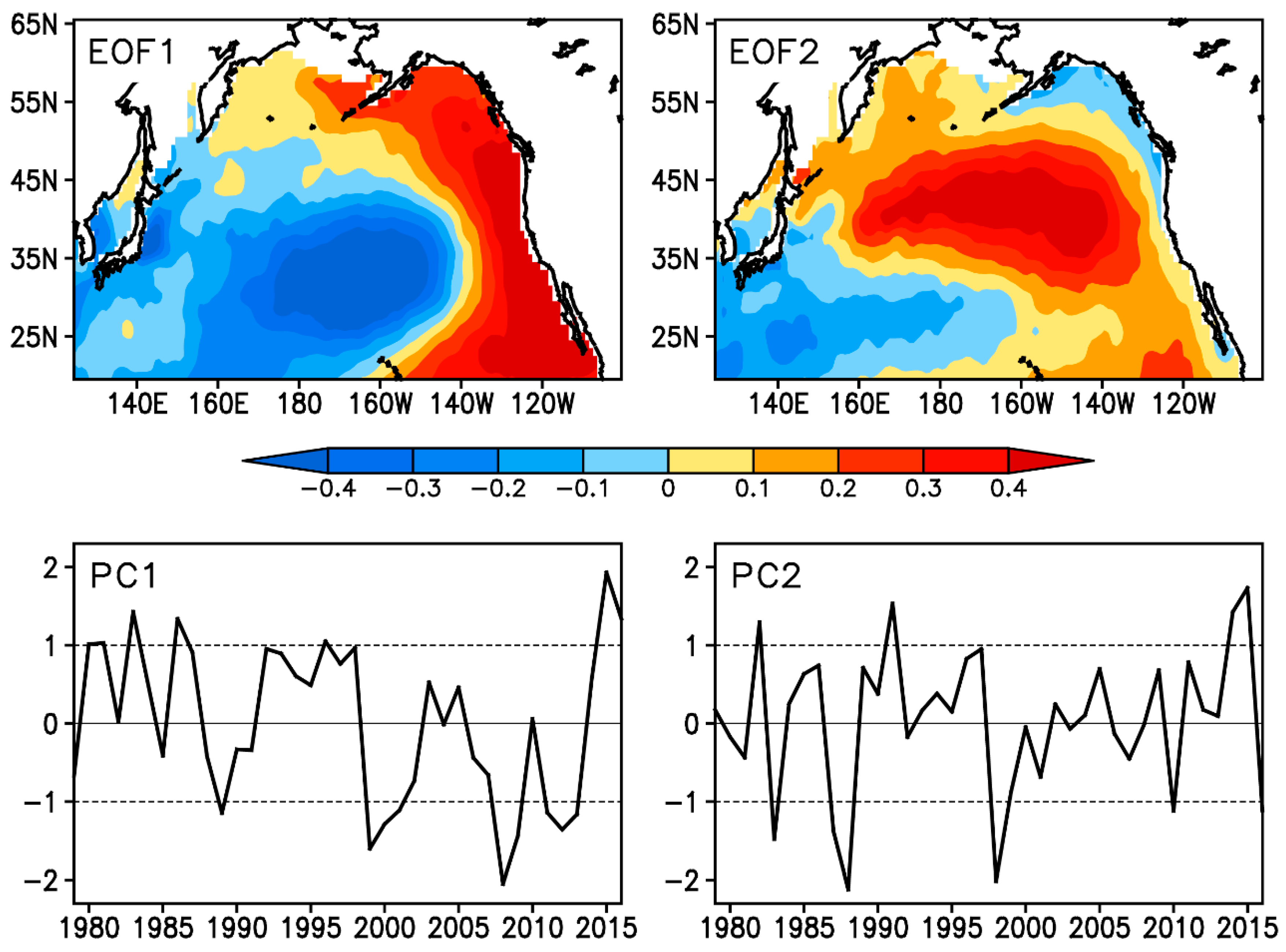
The SCSSM index (SCSSMI) used in this study was the meridional shear vorticity index defined by Wang et al. [3]:

SCSSM = U850N (5° N–15° N, 110° E–120° E) − U850 (20° N–25° N, 110° E–120° E),

where the first and second terms on the right-hand side denote the 850-hPa zonal wind averaged over (5° N–15° N, 110° E–120° E) and over (20° N–25° N, 110° E–120° E), respectively. The SCSSMI is a good indicator of SCSSM rainfall and intensity. A positive (negative) index is associated with an anomalous cyclone (anticyclone) at 850 hPa in the northern SCS, enhanced (reduced) rainfall over the central-northern SCS, and hence a strong summer monsoon (Figure 1). The western North Pacific summer monsoon (WNPSM) index (WNPSMI) was defined by the differences in the 850-hPa zonal wind averaged over (5° N–15° N, 100° E–130° E) and over (20° N–30° N, 110° E–140° E) [33].

2.4. The VM Index

Previous studies reported that the VM is an SST footprint forced by the North Pacific Oscillation (NPO)-like atmospheric variability [28]. The NPO is strongest in winter (December–February (DJF)) [34], while the VM reaches peak around spring (February–April (FMA)) as a delayed response to the NPO forcing [28]. Therefore, we performed EOF analysis of FMA-averaged SST anomalies over the North Pacific poleward of 20° N (after removing the global mean SST anomaly) (Figure 2). The leading EOF mode (EOF1), which explains 27.3% of the total variance, exhibit a basin-wide horseshoe-like spatial pattern over the North Pacific, with SST anomalies of one sign in the western and central North Pacific surrounded by anomalies of the opposite sign along the west coast of North America. This mode is conventionally referred to as the Pacific decadal Oscillation (PDO) [35,36]. The EOF2, which explains 14.2% of the total variance, exhibits a tilted SST anomaly dipole pattern oriented in the northeast–southwest direction, characterized by a band of positive SST anomalies in the northeastern North Pacific and a band of negative SST anomalies extending from the central North Pacific to the WNP. This mode is referred to as the so-called VM [26,27,28]. The VM index (VMI) is defined as the second principal component (PC2) time series associated with the EOF2. A strongly positive (negative) VM case is defined as a year in which the VMI exceeds one positive (negative) standard deviation for the period 1979–2017 (

Table 1. Member years of positive and negative Victoria mode (VM) cases for the period 1979–2017.

Positive VM	1982, 1991, 1997, 2005, 2014, 2015
Negative VM	1983, 1987, 1988, 1998, 1999, 2010, 2016

).

2.5. Statistical Methods

For this study, the statistical significance of correlation, regression, and composite values is determined based on a two-tailed Student t-test and the effective number of degrees of freedom $N_{eff}$. $N_{eff}$ was estimated using the following approximation [37,38]:

$$N_{eff}\approx \frac{N}{1+2{\displaystyle \sum _{i=1}^N\frac{N-i}{N}{R}_X(i)R_Y(i)}}$$

(1)

where $N$ is the total number of available time steps and $R_X(i)$ and $R_Y(i)$ are the autocorrelations of the two sampled time series $X(i)$ and $Y(i)$ ($i$ = 1,…, $N$), respectively.

3. Results

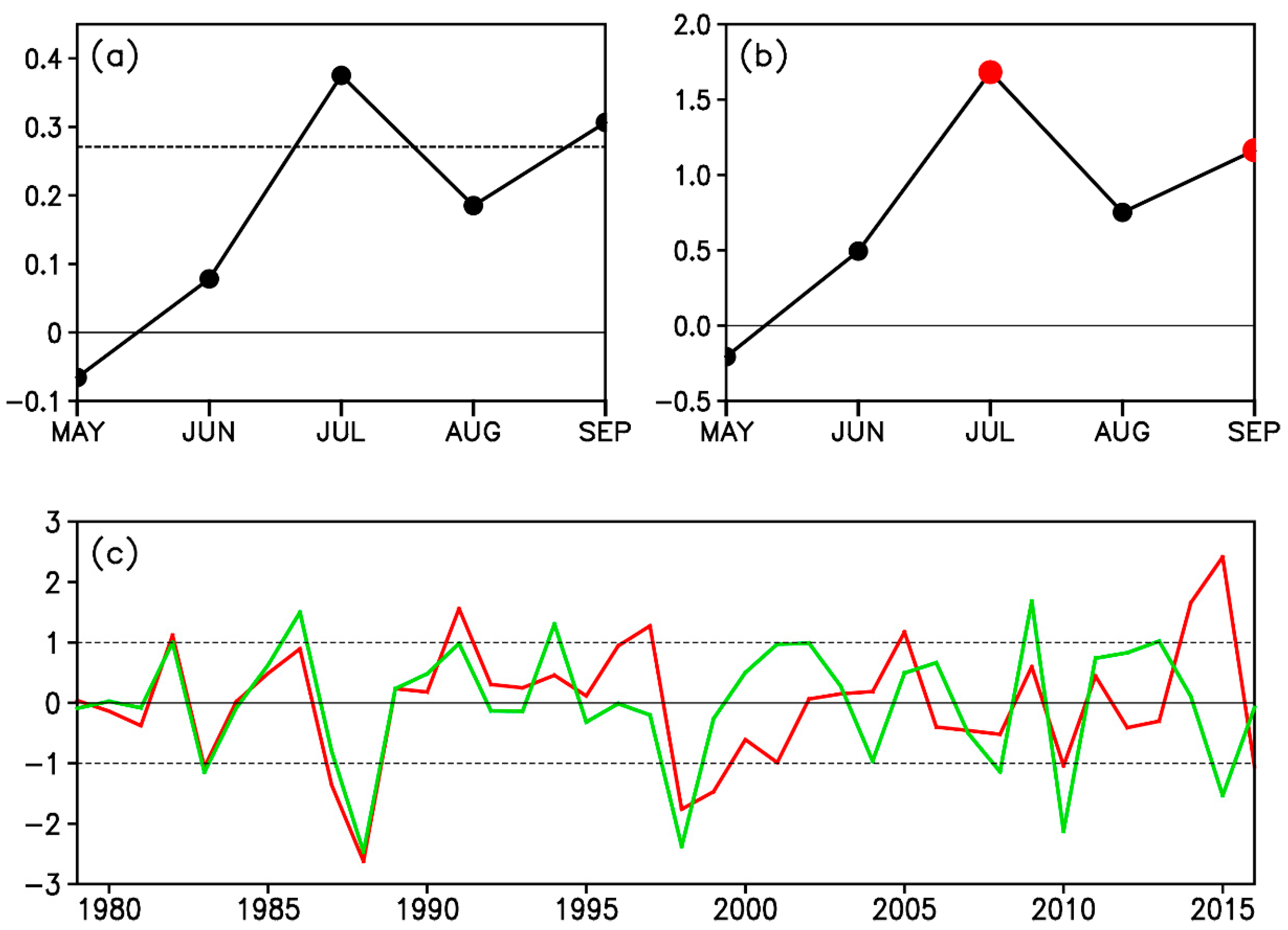
3.1. Relationship Between the VM and SCSSM

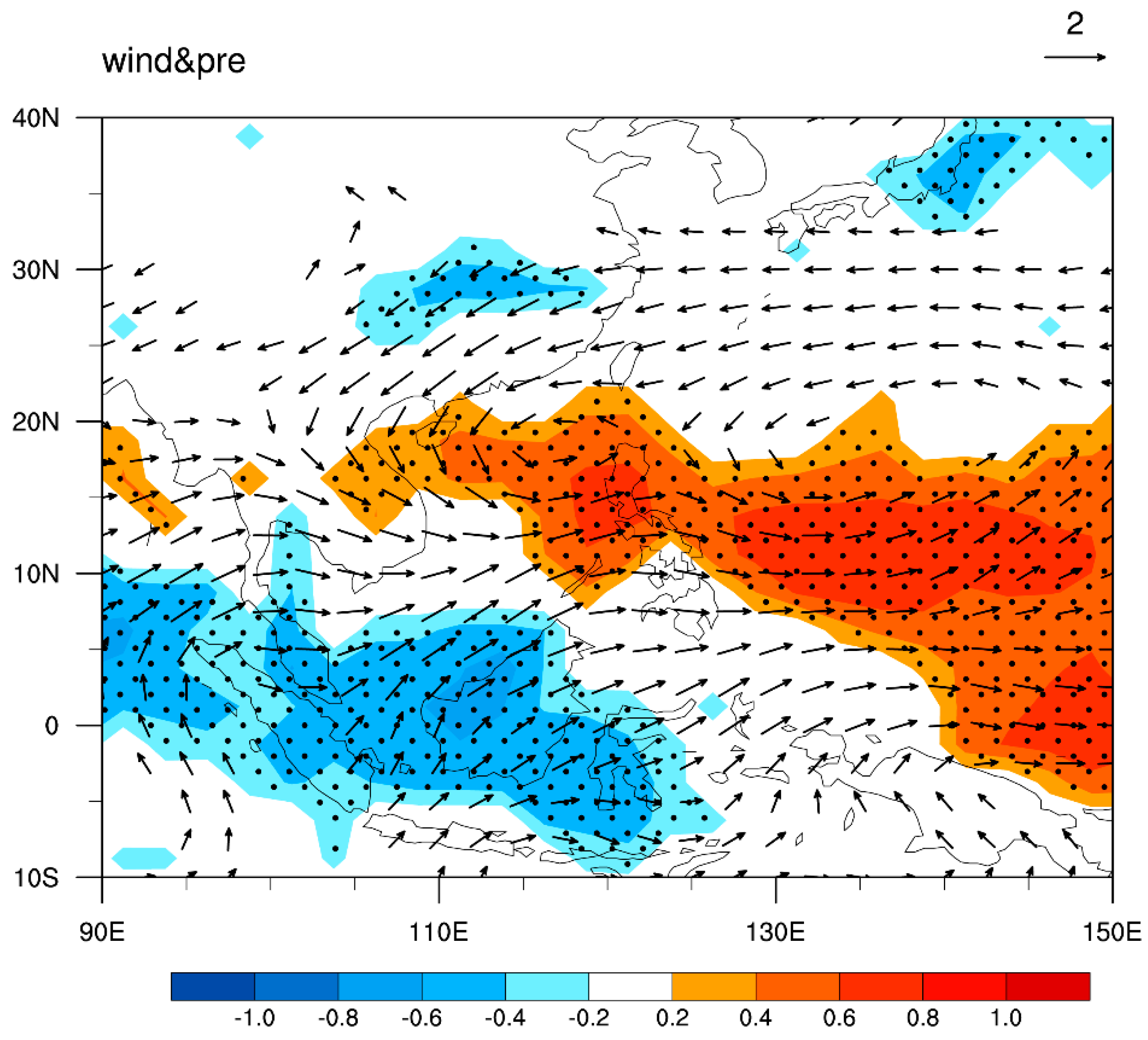
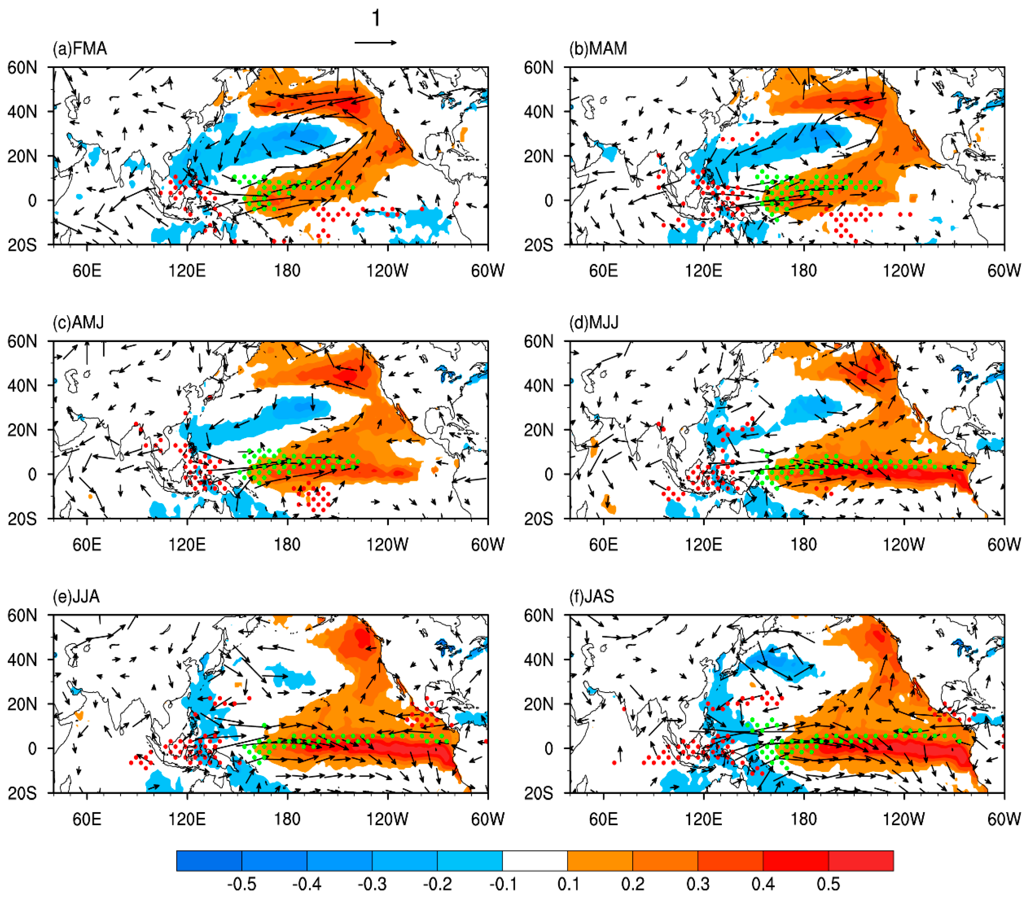
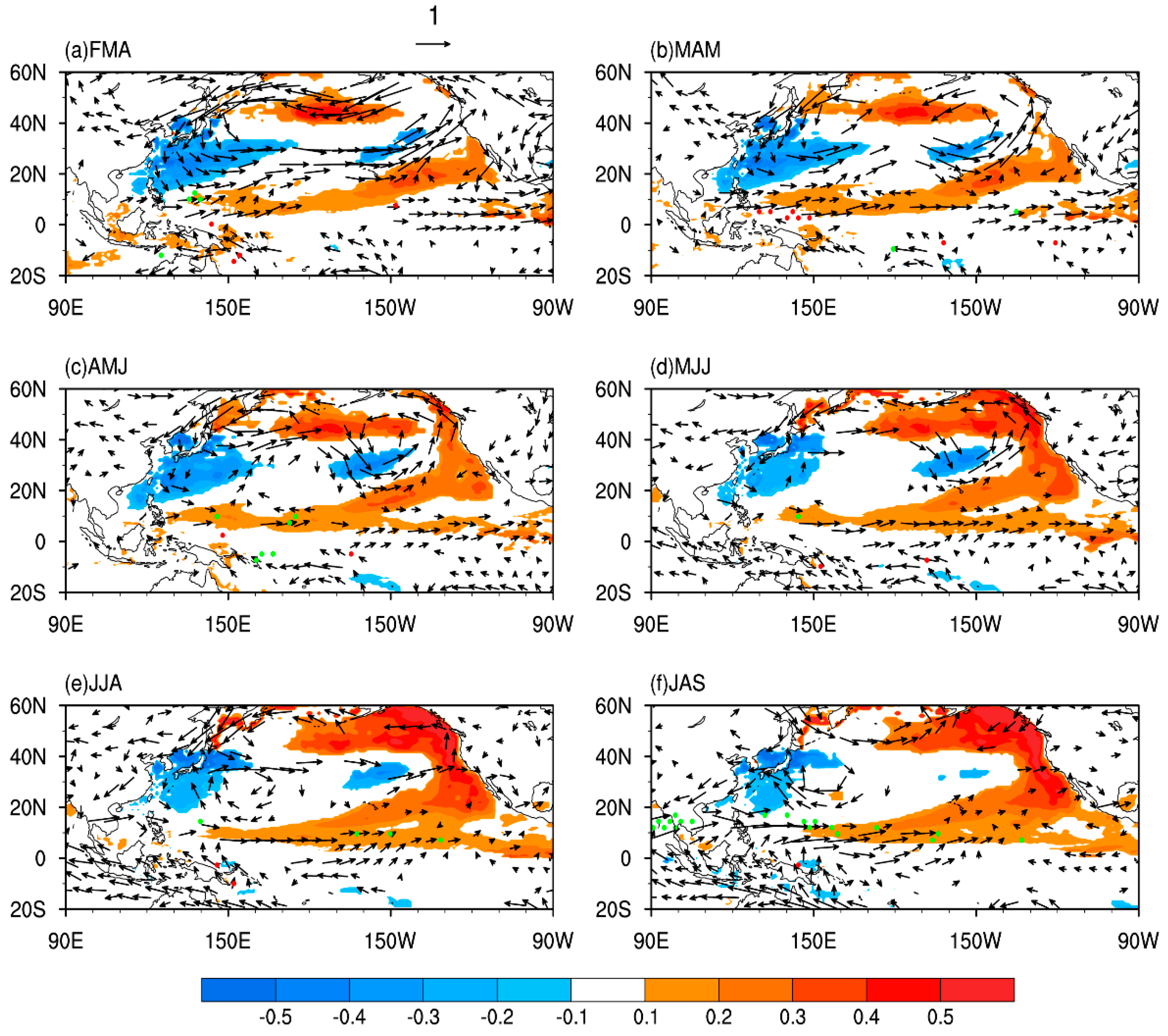
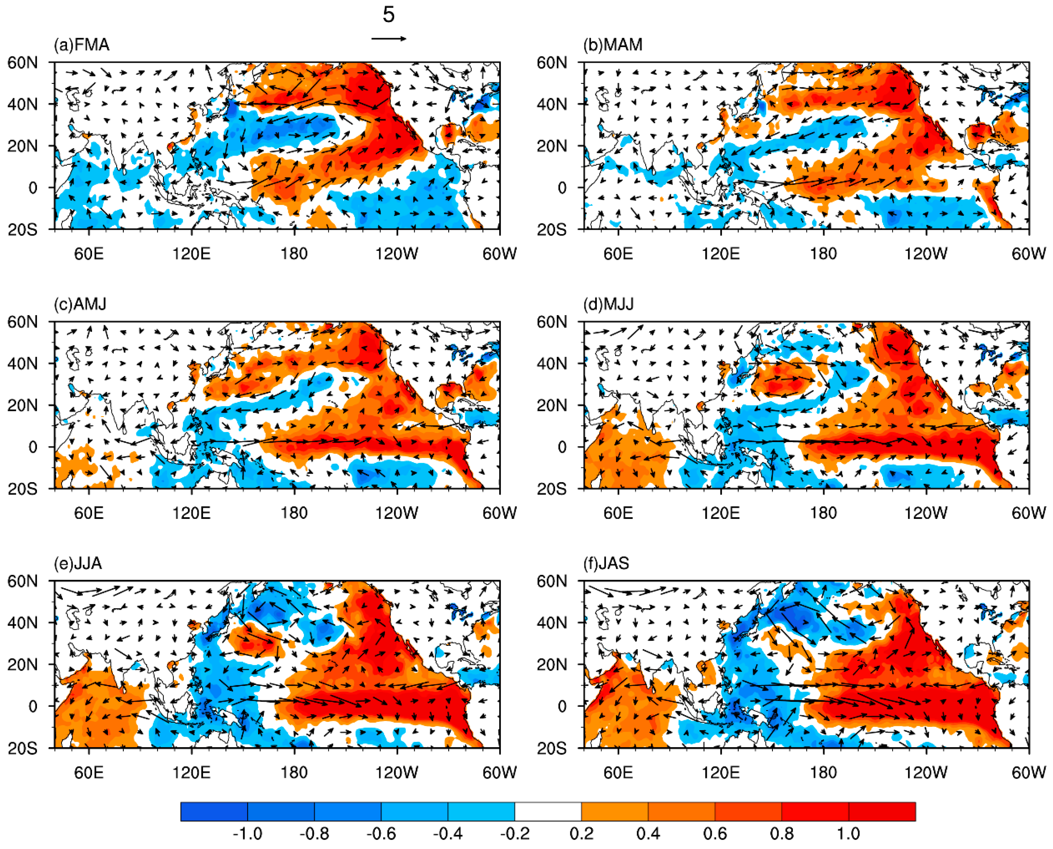
Considering that the SCSSM typically begins around mid-May and retreats around September [3,39,40], we first computed the correlations of the FMA VMI with monthly SCSSMI from May to September (Figure 3a). The correlation is relatively weak in May and June, but increases rapidly after July, and reaches (and even exceeds) the 90% confidence level through September. Figure 3b shows the composite differences in the monthly evolution of the SCSSMI between strongly positive and negative VM cases. It shows that the strongly positive VM cases are followed by significant positive values of the SCSSMI in July and September, consistent with the correlation analysis. Figure 3c shows the time series of the FMA VMI and the following July–September (JAS) SCSSMI. Their correlation is 0.46 (significant at the 99% confidence level), slightly higher than the correlation (0.40, significant at the 95% confidence level) of the FMA VMI with the June–September (JJAS) SCSSMI. These results suggest that the FMA VMI is more strongly correlated with the SCSSMI at the later stage of the SCSSM (the JAS season) than at its early stage (May–June).

To further elaborate the lagged relationship between the VM and SCSSM, we performed a singular value decomposition (SVD) analysis [41] of the cross-covariance matrix between the FMA SST anomalies in the North Pacific (20° N–65° N, 125° E–100° W) and the JAS precipitation anomalies in the SCS monsoon region (0°–22° N, 110° E–120° E). The leading SVD mode accounts for about 51% of the total squared covariance between the two fields. The correlation coefficient between the corresponding expansion coefficients is 0.67 (significant at the 99.9% confidence level) (Figure 4c), indicating that the two fields included in the SVD are strongly coupled. The expansion coefficients of the two fields have strong correlations of 0.94 and 0.61, respectively, with the FMA VMI and JAS SCSSMI. This suggests that these two SVD time series are closely linked to variations in the intensity of the VM and SCSSM, respectively.

The FMA North Pacific SST pattern of the leading SVD mode is characterized by the signature of the VM with significantly positive correlations in the northeastern North Pacific and significantly negative correlations extending from the central North Pacific to the WNP (Figure 4a). The summer precipitation pattern in the SCS for the leading SVD mode shows positive (but not significant) correlations in the central-northern SCS and significantly negative correlations in the southern SCS (Figure 4b), closely resembling the SCSSM-related precipitation pattern in Figure 1. These patterns indicate that a strong VM in late winter and early spring will be followed by an increased (reduced) summer precipitation in the central-northern SCS (in the southern SCS) and thus a strong SCS monsoon. These results are generally consistent with the conclusions from Figure 3 and further confirm the strong lagged relationship between the VM and SCSSM.

Given that ENSO has a significant influence on the SCSSM [3,10,11,12,13,14], the question naturally arises as to whether ENSO could also have an impact on the relationship between the VM and SCSSM. To answer this question, we computed the partial correlation between the FMA VMI and the following JAS SCSSMI by removing the effect of the previous winter (DJF)’s ENSO signal (represented by the Niño3.4 index). The removal of the ENSO signal only reduces the correlation from 0.46 to 0.38 (still significant at the 95% confidence level), indicating that the relationship between the VM and SCSSM is weakly affected by (or relatively independent of) previous winter’s ENSO. Therefore, the springtime VM may be regarded as an independent predictor for the SCSSM’s intensity.

3.2. Mechanisms

We have demonstrated that the springtime VM is closely linked to the SCS summer (JAS) monsoon’s intensity. Next it is necessary to examine the underlying mechanisms through which the VM affects the SCSSM. The mechanisms by which the extratropical atmospheric variability over the North Pacific influences the tropical Pacific SST anomalies have been extensively discussed [42,43,44,45,46,47]. It is proposed that the extratropical atmospheric variability can initiate a basin-scale SST structure via modifying the wind-stress field and in turn net surface heat flux. This SST footprint, which is referred to as the VM, reaches a maximum in spring, and persists until summer via the wind-evaporation-SST (WES) feedback [48] in the subtropics (5°–20° N). These persistent subtropical SST anomalies can then force the overlying atmosphere to initiate tropical SST anomalies (the seasonal footprinting mechanism) [43,44].

To examine the impact of the VM on SST, precipitation, and surface wind anomalies over the SCS, lagged regressions are calculated with respect to the FMA VMI (Figure 5). During spring (MAM), the VM is associated with a basin-wide tripole SST anomaly pattern in the North Pacific, with a band of positive SST anomalies extending from the west coast of North America to the central equatorial Pacific, a band of negative SST anomalies extending from the central North Pacific to the WNP, and another band of positive SST anomalies in the Pacific north of 35° N. At this time, the SST anomaly pattern associated with the VM in the tropical central eastern Pacific bears a resemblance to a Pacific meridional mode (PMM) pattern, with positive SST anomalies in the northeastern subtropical Pacific and negative SST anomalies in the equatorial eastern Pacific, indicating that the VM is closely linked to the PMM. However, we would like to emphasize that the VM is a basin-scale North Pacific SST pattern. In addition to the PMM pattern, there are significant negative SST anomalies associated with the VM in the WNP. The WNP SST anomalies have been shown to have an important contribution independent of the PMM to the initiation of ENSO events [49]. Therefore, in contrast to the local influence of the PMM, the VM may play a unique role (i.e., as a basin-scale influence) in affecting the tropical Pacific climate [28].

During summer (JJA), negative (positive) SST anomalies in the central North Pacific (in the high-latitude North Pacific) gradually decay. Instead, SST anomalies in the subtropical North Pacific persist until summer and develop toward the equator via the seasonal footprinting mechanism, resulting in significant positive SST anomalies in the central-eastern equatorial Pacific and significant negative SST anomalies in the WNP. The SST warming in the central-eastern equatorial Pacific and the cooling in the WNP weaken the zonal SST gradient across the WNP to central equatorial Pacific, which in turn induces the anomalous westerlies in the western equatorial Pacific. These anomalous westerlies cause low-level divergence and convergence respectively over the Maritime Continent and central equatorial Pacific, thereby leading to enhanced (suppressed) convection and precipitation over the central equatorial Pacific (over the Maritime Continent) [27]. At the same time, the diabatic heating associated with precipitation anomalies induces a low-level cyclonic flow over the WNP as a Gill-type Rossby-wave response [50], which in turn gives rise to a westerly flow on its south flank (see also Figure 6 for the results from a simple numerical experiment using the Matsuno-Gill model). This westerly flow enhances the anomalous westerlies in the western equatorial Pacific, which reinforces the positive (negative) precipitation anomalies over the central equatorial Pacific (over the Maritime Continent). This positive feedback process among SST, precipitation, and zonal stress in the western tropical Pacific helps to amplify and sustain the anomalous cyclone over the WNP during the JAS season, leading to a strong WNPSM over the Philippine Sea. When the WNPSM is strong, the SCSSM is also intensified because of the robust in-phase relation between the WNPSM and SCSSM [3], as confirmed by significant positive correlations between the WNPSM and SCSSM indices (R = 0.95, significant at the 99.9% confidence level) and between the FMA VMI and the JAS WNPSMI (R = 0.49, significant at the 99% confidence level). We note that significant precipitation anomalies associated with the VM during JAS are mainly located over the Maritime Continent, and there is really a precipitation response to the VM in the SCS but this response is relatively weak (not significant) (Figure 5f).

To further elucidate the effect of the VM-related SST anomalies on the SCSSM, two numerical experiments using the FGOALS-g2 are performed with and without the VM-related SST anomalies in the North Pacific (denoted as the forcing and control experiments, respectively). The VM-related SST anomalies in the North Pacific poleward of 10° N are obtained from regressions of the FMA SST anomalies onto the concurrent VMI (not shown). The control run was integrated for 23 years and forced with the climatological SST, and the last 12 years were used to provide the basic annual mean state. The forcing experiment was integrated for 18 years and forced with the VM-related SST anomalies imposed on the climatological SST, and the last 12 years were used in the composite analysis. The composite differences in the seasonal evolution of SST, precipitation, and surface wind anomalies between the forcing and control experiments are shown in Figure 7. The results from the CGCM experiments confirm that the VM-related North Pacific SST anomalies during FMA can extend to tropics during the following summer that subsequently lead to the development of the anomalous cyclone over the SCS. It can also be seen that the anomalous westerly flow is significant in the central and southern SCS, which implies that the SCSSM is intensified. These simulated results are almost consistent with the observation (Figure 5), and further indicate that the VM may play an important role in influencing the SCSSM’s intensity.

The results described above reveal the mechanism through which the VM affects the SCSSM. However, it should be noted that some strong VM events are not followed by the SCSSMI of the same sign (Figure 3c). For example, 2015 was such a year in which the FMA VMI was 2.4 (one of the strongest VM events on record [51]), while the JAS SCSSMI was −1.5. In addition, 1997 was also a typical year in which a positive VM event is followed by a weak SCSSM (the FMA VMI and the JAS SCSSMI were 1.28 and −0.20, respectively). It is important to understand why the VM is ineffective in affecting the SCSSM in these years. By examining the seasonal evolution of SST and 850 hPa wind anomalies in 2015 (Figure 8), it is found that an El Niño event followed by a strong VM is developing in the tropical Pacific during summer. But at the same time, a strong Indian Ocean dipole (IOD) event (positive SST anomalies in the western Indian Ocean and negative SST anomalies in the eastern Indian Ocean south of Indonesia) [52] is also happening in the tropical Indian Ocean. It has been reported in a previous study that a moderate positive IOD event occurred in 2015 concurrent with the 2015/2016 extreme El Niño [53]. The IOD-related dipole SST pattern is associated with the anomalous easterly in the equatorial Indian Ocean and the southern SCS, thereby possibly leading to a weak SCSSM. Similarly, 1997 was also a strong positive IOD event co-occurring with an extreme El Niño in which the relationship between the VM and SCSSM broke down. These results suggest that the influences of the VM on the SCSSM may be weakened in some years by the interference between the IOD and El Niño when an El Niño and a positive IOD event (or a La Niña and a negative IOD event) co-occur. Moreover, the VMI accounts for only about 15% of the variance of the SCSSMI. Therefore, when considering the influence of the VM on the SCSSM, we cannot exclude the role of other possible factors, such as the IOD. Further study is required to examine the joint effect of the VM and other factors on the SCSSM, which may substantially contribute to the prediction of the SCSSM.

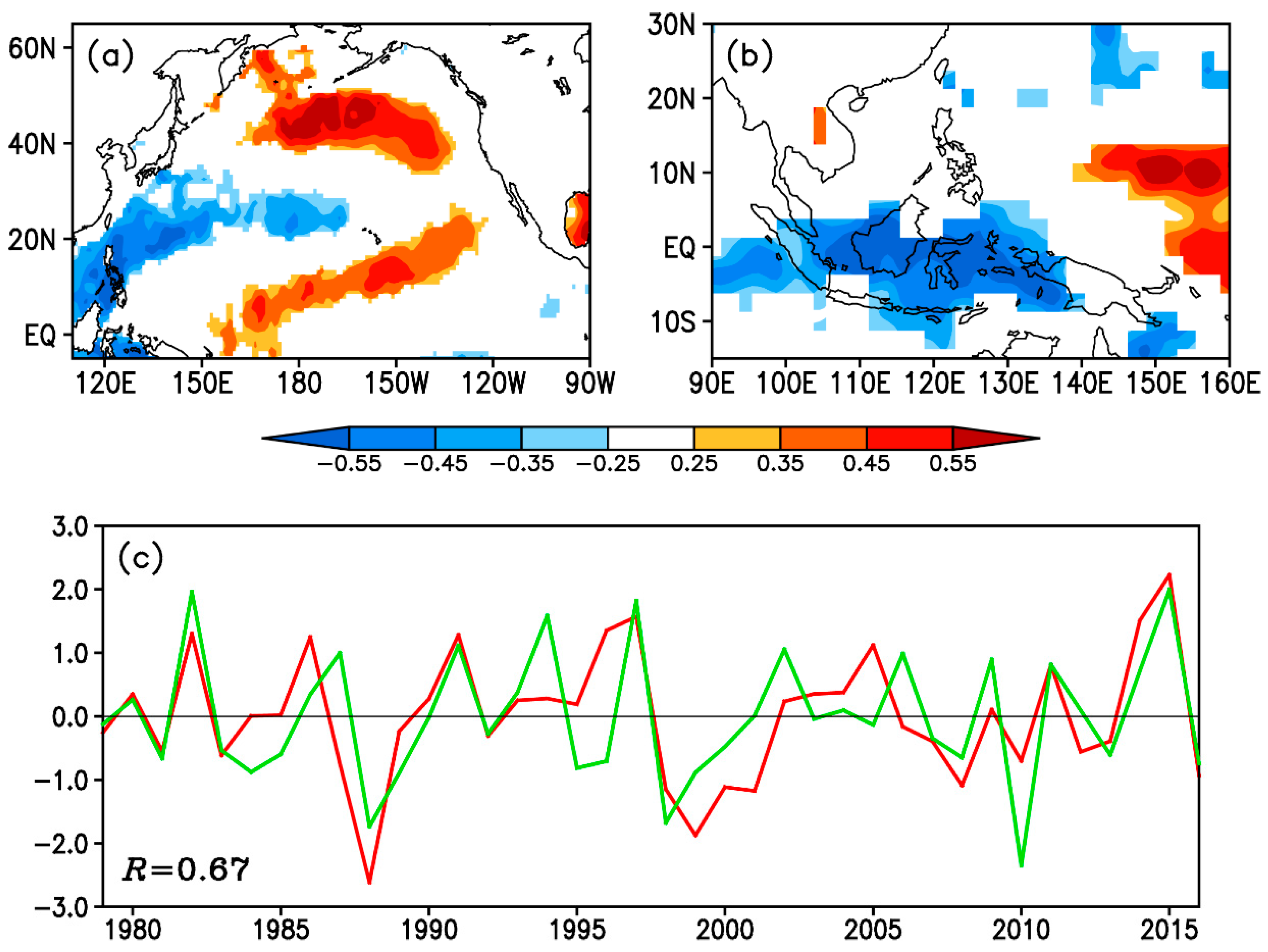
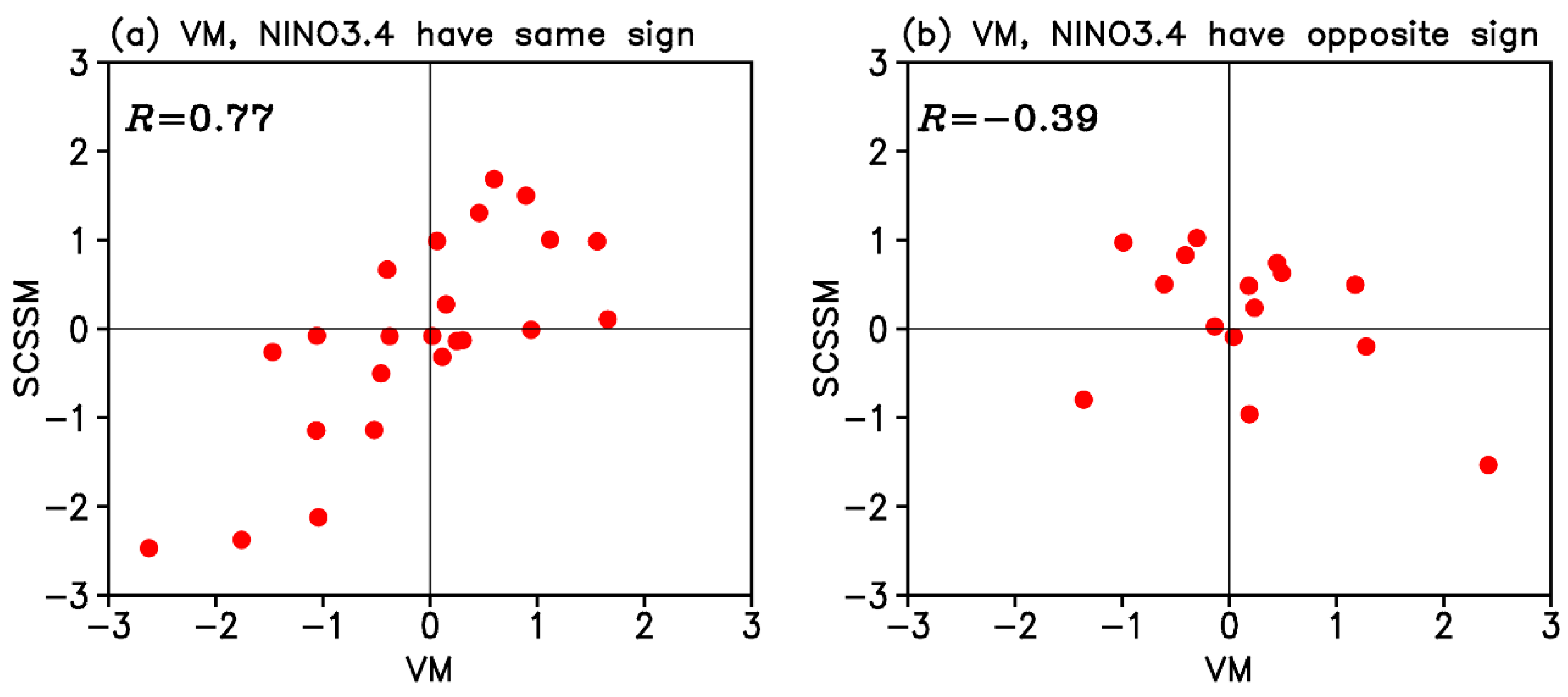
3.3. Linkage Among the VM, SCSSM, and ENSO

The above analysis suggests that the VM has a significant influence on the SCSSM. Previous studies reported that the VM also plays an important role in initiating ENSO. Given that the VM can affect both the SCSSM and ENSO, we may wonder whether there is any linkage between influences of the VM on the SCSSM and ENSO. As shown in Figure 5, the VM-related SST warming in the central-eastern equatorial Pacific induces an anomalous westerly in the western equatorial Pacific that in turn influences the SCSSM. Conversely, the reduced convective precipitation and latent heat release in the southern SCS associated with the SCSSM may cause an intensification of low-level divergence there and hence strengthened westerlies in the western equatorial Pacific, which are conducive to the development of an El Niño event.

We investigated the joint relation among the VM, SCSSM, and ENSO through a scatterplot between the FMA VMI and the following JAS SCSSMI, stratified by whether the FMA VMI has the opposite or the same sign as the following DJF Niño3.4 index (Figure 9). We noted that the correlation between the VM and SCSSM indices is high (R = 0.77; significant at the 99.9% confidence level) when the VM and Niño3.4 indices have the same sign (Figure 9a), while the correlation is only −0.39 (not significant even at the 90% confidence level) when the VMI is opposite to the Niño3.4 index (Figure 9b). These results suggest that the processes in the tropical Pacific involved in the VM influence on ENSO may be inherently linked to those involved in its influence on the SCSSM. If the VM cannot induce an ENSO event in the following winter, there is a much higher probability that the VM is also ineffective in influencing the SCSSM. Similar results are obtained when the FMA VMI and the following DJF Niño3.4 index are conditioned upon whether they have the same or opposite sign (not shown), suggesting that the influence of the VM on ENSO also depends on its influence on the SCSSM.

Previous studies have shown that the relationship between ENSO and the SCSSM is an interactive process. ENSO not only influences the SCSSM during its developing phase, but is also affected by the SCSSM-related westerly anomalies in the western equatorial Pacific during its developing phase [54,55]. Our results suggest that the interactive relationship between ENSO and the SCSSM may partly arise from the mutual influence of the VM on both ENSO and the SCSSM through the VM-related westerly anomalies in the western equatorial Pacific. Therefore, a systematic dynamic link among the VM, SCSSM, and ENSO may exist: $\mathrm{VM}(\mathrm{spring})\to \mathrm{SCSSM}(\mathrm{summer})\rightleftarrows \mathrm{ENSO}(\mathrm{winter})$. It follows that the SCSSM plays an important role in linking the VM to ENSO. Furthermore, our study also suggests that the precursor SST pattern of ENSO is similar to that of the SCSSM. In addition to the VM-related SST pattern in the North Pacific, southern Indian Ocean SST anomalies [56], northern tropical Atlantic SST anomalies [57,58], and a quadrapole SST pattern in the extratropical South Pacific [59,60] have been identified as useful precursors for ENSO events. All of these factors have been shown to affect ENSO mainly via influencing the anomalous cyclonic circulation over the WNP and wind anomalies over the western equatorial Pacific. Meanwhile, we note that these factors could also serve as important precursors for the SCSSM (Figure 10), which provides further evidence that influences of these preceding signals on ENSO may be closely related to their influences on the SCSSM.

4. Summary and Discussion

This study has explored the lagged relationship between the VM and SCSSM. Our results have indicated that the VM may significantly affect the interannual variations of the SCSSM’s intensity, as supported by significant positive correlations between the FMA VMI and the following JAS SCSSMI. It appears that the SCSSM tends to strengthen when the springtime VM is stronger than normal. This influence of the VM on the SCSSM’s intensity is relatively independent of the previous winter’s ENSO influence on the SCSSM’s intensity.

The present analysis reveals that the VM exerts an effect on the SCSSM’s intensity mainly via the so-called seasonal footprinting mechanism. That is, SST anomalies in the subtropics associated with the springtime VM persist into summer and develop gradually toward the equator, resulting in a weakened zonal SST gradient across the WNP to the central equatorial Pacific. Then, changes in the zonal SST gradient in the tropical Pacific produce an anomalous cyclonic flow over the WNP and westerly anomalies in the western equatorial Pacific, thereby intensifying the WNPSM as well as the SCSSM (see Figure 11 for a schematic diagram). At the same time, the VM-induced wind stress anomalies in the western equatorial Pacific are conducive to initiating an ENSO event. Therefore, the VM influence on both the WNPSM and SCSSM is simultaneously associated with its influence on ENSO, indicating that the VM may serve as a useful predictor to enhance predictive skill of both the SCS-WNP summer monsoon and ENSO.

Recent studies reported a pronounced strengthening of the VM since 1990 [26,28,61]. This recent strengthening of the VM may be attributed to a response of North Pacific climate system to anthropogenic forcing and global warming [61]. If global warming will continue, the VM may be expected to play an increasingly important role in influencing the SCS-WNP summer monsoon in coming decades. Further work is needed to explore the long-term variations of the VM itself, as well as its role in affecting the tropical climate system’s variability and predictability.

References

1. Tao, S.; Chen, L. A review of recent research on the East Asian summer monsoon in China. In Monsoon Meteorology; Oxford University Press: Tokyo, Japan, 1987; pp. 60–92. [Google Scholar]
2. Ding, Y.; Li, C.; Liu, Y. Overview of the South China Sea Monsoon Experiment. Adv. Atmos. Sci. 2004, 21, 343–360. [Google Scholar]
3. Wang, B.; Huang, F.; Wu, Z.; Yang, J.; Fu, X.; Kikuchi, K. Multi-scale climate variability of the South China Sea monsoon: A review. Dyn. Atmos. Oceans 2009, 47, 15–47. [Google Scholar] [CrossRef]
4. Murakami, T.; Matsumoto, J. Summer monsoon over the Asian continent and western north Pacific. J. Meteorol. Soc. Jpn. 1994, 72, 719–745. [Google Scholar] [CrossRef]
5. Wu, R.; Wang, B. Multi-stage onset of the summer monsoon over the western North Pacific. Clim. Dyn. 2001, 17, 277–289. [Google Scholar] [CrossRef]
6. Wang, B.; LinHo, L.H. Rainy season of the Asian–Pacific summer monsoon. J. Clim. 2002, 15, 386–398. [Google Scholar] [CrossRef]
7. Chen, L.; Zhang, B.; Zhang, Y. Progress in research on the East Asian Monsoon. J. Appl. Meterol. Sci. 2006, 17, 711–724. [Google Scholar]
8. Lau, K.; Yang, S. Climatology and interannual variability of the Southeast Asian summer monsoon. Adv. Atmos. Sci. 1997, 14, 141–162. [Google Scholar] [CrossRef]
9. Mao, J.; Chan, J.; Wu, G. Interannual variations of early summer monsoon rainfall over south China different PDO backgrounds. Int. J. Climatol. 2001, 31, 847–862. [Google Scholar] [CrossRef]
10. Wang, B.; Yang, J.; Zhou, T. Interdecadal changes in the major modes of Asian–Australian monsoon variability: Strengthening relationship with ENSO since the late 1970s. J. Clim. 2008, 21, 1771–1789. [Google Scholar] [CrossRef]
11. Chan, J.; Zhou, W. PDO, ENSO and the early summer monsoon rainfall over south China. Geophys. Res. Lett. 2005, 32, 93–114. [Google Scholar] [CrossRef]
12. Zhou, W.; Chan, J. ENSO and the South China Sea summer monsoon onset. Int. J. Climatol. 2007, 27, 157–167. [Google Scholar] [CrossRef] [Green Version]
13. Luo, M.; Leung, Y.; Graf, H.; Herzog, M.; Zhang, W. Interannual variability of the onset of the South China Sea summer monsoon. Int. J. Climatol. 2015, 36, 550–562. [Google Scholar] [CrossRef] [Green Version]
14. Ge, F.; Zhi, X.; Babar, A.; Tang, W.; Chen, P. Interannual variability of the summer monsoon precipitation over the Indochina Peninsula in association with ENSO. Theor. Appl. Climatol. 2017, 128, 523–531. [Google Scholar] [CrossRef]
15. Wang, B.; Wu, R.; Fu, X. Pacific-East Asian teleconnection: How does ENSO affect East Asian Climate? J. Clim. 2000, 13, 1517–1536. [Google Scholar] [CrossRef]
16. Xie, S.; Hu, K.; Hafner, J.; Tokinaga, H.; Du, Y.; Huang, G.; Sampe, T. Indian Ocean capacitor effect on Indo-western Pacific climate during the summer following El Niño. J. Clim. 2009, 22, 730–747. [Google Scholar] [CrossRef]
17. Stuecker, M.; Jin, F.; Timmermann, A.; McGregor, S. Combination mode dynamics of the anomalous Northwest Pacific anticyclone. J. Clim. 2015, 28, 1093–1111. [Google Scholar] [CrossRef]
18. Li, C.; Mu, M. The influence of the Indian Ocean dipole on atmospheric circulation and climate. Adv. Atmos. Sci. 2001, 18, 831–843. [Google Scholar]
19. Yuan, Y.; Yang, H.; Zhou, W.; Li, C. Influences of the Indian Ocean dipole on the Asian summer monsoon in the following year. Int. J. Climatol. 2008, 28, 1849–1859. [Google Scholar] [CrossRef] [Green Version]
20. Ding, R.; Ha, K.; Li, J. Interdecadal shift in the relationship between the East Asian summer monsoon and the tropical Indian Ocean. Clim. Dyn. 2010, 34, 1059–1071. [Google Scholar] [CrossRef]
21. He, Z.; Wu, R. Indo-Pacific remote forcing in summer rainfall variability over the South Pacific Sea. Clim. Dyn. 2014, 42, 2323–2337. [Google Scholar] [CrossRef]
22. Wu, R. Subseasonal variability during the South China Sea summer monsoon onset. Clim. Dyn. 2010, 34, 629–642. [Google Scholar] [CrossRef]
23. He, Z.; Wu, R. Seasonality of interannual atmosphere-ocean interaction in the South China Sea. J. Oceanogr. 2013, 69, 699–712. [Google Scholar] [CrossRef]
24. Lin, A.; Gu, D.; Zheng, B.; Li, C.; Ji, Z. Relationship between South China Sea summer monsoon onset and Southern Ocean sea surface temperature variation. Chin. J. Geophys. 2017, 56, 383–391. [Google Scholar]
25. Liu, T.; Li, J.; Li, Y.; Zhao, S.; Zheng, F.; Zheng, J.; Yao, Z. Influence of the May Southern annular mode on the South China Sea summer monsoon. Clim. Dyn. 2017, 1–13. [Google Scholar] [CrossRef]
26. Bond, N.; Overland, J.; Spillane, M.; Stabeno, P. Recent shifts in the state of the North Pacific. Geophys. Res. Lett. 2003, 30, 2183. [Google Scholar] [CrossRef]
27. Ding, R.; Li, J.; Tseng, Y.; Yuan, C. Influence of the North Pacific Victoria mode on the Pacific ITCZ summer precipitation. J. Geophys. Res. 2015, 120, 964–979. [Google Scholar] [CrossRef] [Green Version]
28. Ding, R.; Li, J.; Tseng, Y.; Sun, C.; Guo, Y. The Victoria mode in the North Pacific linking extratropical sea level pressure variations to ENSO. J. Geophys. Res. 2015, 120, 27–45. [Google Scholar] [CrossRef] [Green Version]
29. Kanamitsu, M.; Ebisuzaki, W.; Woollen, J.; Yang, S.; Sling, J.; Fiorino, M.; Potter, G. NCEP-DOE AMIP-II Reanalysis (R-2). Bull. Am. Meteorol. Soc. 2002, 83, 1631–1643. [Google Scholar] [CrossRef]
30. Smith, T.; Reynolds, R.; Peterson, T.; Lawrimore, J. Improvements to NOAA’s historical merged land-ocean surface temperature analysis (1880–2006). J. Clim. 2008, 21, 2283–2296. [Google Scholar] [CrossRef]
31. Xie, P.; Arkin, P. Global precipitation: A 17-year monthly analysis based on gauge observations, satellite estimates, and numerical model outputs. Bull. Am. Meteorol. Soc. 1997, 78, 2539–2558. [Google Scholar] [CrossRef]
32. Li, L.J.; Lin, P.F.; Yu, Y.Q.; Wang, B.; Zhou, T.J.; Liu, L.; Liu, J.P.; Bao, Q.; Xu, S.M.; Huang, W.Y.; et al. The Flexible Global Ocean-atmosphere-land System Model, Grid-point Version 2: FGOALS-G2. Adv. Atmos. Sci. 2013, 30, 543–560. [Google Scholar] [CrossRef]
33. Wang, B.; Wu, R.; Lau, K. Interannual variability of the Asian summer monsoon: Contrasts between the Indian and the western North Pacific-East Asian monsoons. J. Clim. 2001, 14, 4073–4090. [Google Scholar] [CrossRef]
34. Rogers, J. The North Pacific Oscillation. J. Climatol. 1981, 1, 39–57. [Google Scholar] [CrossRef]
35. Mantua, N.; Hare, S.; Zhang, Y.; Wallace, J.; Francis, R. A Pacific interdecadal climate oscillation with impacts on salmon production. Bull. Am. Meteorol. Soc. 1997, 78, 1069–1079. [Google Scholar] [CrossRef]
36. Zhang, Y.; Wallace, J.; Battisti, D. ENSO-like interdecadal variability. J. Clim. 1997, 10, 1004–1020. [Google Scholar] [CrossRef]
37. Pyper, B.; Peterman, R. Comparison of methods to account for autocorrelation in correlation analyses of fish data. Can. J. Fish. Aquat. Sci. 1998, 55, 2127–2140. [Google Scholar] [CrossRef]
38. Li, X.; Yu, J.; Li, Y. Recent summer rainfall increase and surface cooling over Northern Australia: A response to warming in the tropical Western Pacific. J. Clim. 2013, 26, 7221–7239. [Google Scholar] [CrossRef]
39. Wang, B.; Lin, H.; Zhang, Y.; Lu, M. Definition of South China sea monsoon onset and commencement of the east Asia summer monsoon. J. Clim. 2004, 17, 699–710. [Google Scholar] [CrossRef]
40. Shin, C.; Huang, B. Slow and fast annual cycles of the Asian summer monsoon in the NCEP CFSv2. Clim. Dyn. 2016, 47, 529–553. [Google Scholar] [CrossRef]
41. Bretherton, C.; Smith, C.; Wallace, J. An intercomparison of methods for finding coupled patterns in climate data. J. Clim. 1992, 5, 541–560. [Google Scholar] [CrossRef]
42. Anderson, B. Tropical Pacific sea-surface temperatures and preceding sea level pressure anomalies in the subtropical North Pacific. J. Geophys. Res. 2013, 108, D23. [Google Scholar] [CrossRef]
43. Vimont, D.; Wallace, J.; Battisti, D. The seasonal footprinting mechanism in the Pacific: Implications for ENSO. J. Clim. 2003, 16, 2668–2675. [Google Scholar] [CrossRef]
44. Vimont, D.; Battisti, D.; Hirst, A. The seasonal footprinting mechanism in the CSIRO general circulation models. J. Clim. 2003, 16, 2653–2667. [Google Scholar] [CrossRef]
45. Alexander, M.; Vimont, D.; Chang, P.; Scott, D. The impact of extratropical atmospheric variability on ENSO: Testing the seasonal footprinting mechanism using coupled model experiments. J. Clim. 2010, 23, 2885–2901. [Google Scholar] [CrossRef]
46. Yu, J.; Kim, S. Relationships between extratropical sea level pressure variations and the central Pacific and eastern Pacific types of ENSO. J. Clim. 2011, 24, 708–720. [Google Scholar] [CrossRef]
47. Ding, R.; Li, J.; Tseng, Y.; Sun, C.; Xie, F. Joint impact of North and South Pacific extratropical atmospheric variability on the onset of ENSO events. J. Geophys. Res. 2017, 122, 279–298. [Google Scholar] [CrossRef]
48. Xie, S.; Philander, S. A coupled ocean–atmosphere model of relevance to the ITCZ in the eastern Pacific. Tellus 1994, 46A, 340–350. [Google Scholar] [CrossRef]
49. Wang, S.; L’Heureux, M.; Chia, H. ENSO prediction one year in advance using western North Pacific sea surface temperatures. Geophys. Res. Lett. 2012, 39, L05702. [Google Scholar] [CrossRef]
50. Gill, A. Some simple solutions for heat-induced tropical circulation. Q. J. R. Meteorol. Soc. 1980, 106, 447–462. [Google Scholar] [CrossRef]
51. Tseng, Y.; Ding, R.; Huang, X. The warm Blob in the northeast Pacific-The bridge leading to the 2015/16 El Niño. Environ. Res. Lett. 2017, 12, 054019. [Google Scholar] [CrossRef]
52. Saji, N.; Goswami, B.; Vinayachandran, P.; Yamagata, T. A dipole mode in the tropical Indian Ocean. Nature 1999, 401, 360–363. [Google Scholar] [CrossRef] [PubMed]
53. Zhang, L.; Du, Y.; Cai, W. Low-frequency variability and the unusual Indian Ocean dipole events in 2015 and 2016. Geophys. Res. Lett. 2018, 45. [Google Scholar] [CrossRef]
54. Huang, R.; Zhang, R.; Yan, B. Dynamical effect of the zonal wind anomalies over the tropical western Pacific on ENSO cycles. Sci. China Earth Sci. 2001, 44, 1089–1098. [Google Scholar] [CrossRef]
55. Wu, R.; Kirtman, B. On the impacts of the Indian summer monsoon on ENSO in a coupled GCM. Q. J. R. Meteorol. Soc. 2003, 129, 3439–3468. [Google Scholar] [CrossRef] [Green Version]
56. Terray, P.; Dominiak, S. Indian Ocean Sea Surface Temperature and El Niño–Southern Oscillation: A New Perspective. J. Clim. 2005, 18, 1351–1368. [Google Scholar] [CrossRef] [Green Version]
57. Ham, Y.; Kug, J.; Park, J.; Jin, F. Sea surface temperature in the north tropical Atlantic as a trigger for El Niño/Southern Oscillation events. Nat. Geosci. 2013, 6, 112–116. [Google Scholar] [CrossRef]
58. Ding, R.; Li, J.; Tseng, Y.; Sun, C.; Zheng, F. Linking a sea level pressure anomaly dipole over North America to the central Pacific El Niño. Clim. Dyn. 2017, 49, 1321–1339. [Google Scholar] [CrossRef]
59. Ding, R.; Li, J.; Tseng, Y. The impact of South Pacific extratropical forcing on ENSO and comparisons with the North Pacific. Clim. Dyn. 2015, 44, 2017–2034. [Google Scholar] [CrossRef]
60. Ding, R.; Li, J.; Tseng, Y.; Ha, J.; Zhao, S.; Lee, J. Interdecadal change in the lagged relationship between the Pacific–South American pattern and ENSO. Clim. Dyn. 2016, 47, 2867–2884. [Google Scholar] [CrossRef]
61. Di Lorenzo, E.; Schneider, N.; Cobb, K.; Franks, P.; Chhak, K.; Miller, A.; McWilliams, J.; Bograd, S.; Arango, H.; Curchitser, E.; et al. North Pacific Gyre Oscillation links ocean climate and ecosystem change. Geophys. Res. Lett. 2008, 35, L08607. [Google Scholar] [CrossRef]
Figure 1. Correlations of summer (June–September (JJAS)) precipitation (shaded) and wind vectors at 850 hPa (vector) with the concurrent South China Sea summer monsoon (SCSSM) index (SCSSMI). Positive (red) and negative (blue) precipitation anomalies, with correlation significant at the 90% confidence level, are stippled. Only wind vectors at 850 hPa with correlation significant at the 90% confidence level are shown.
Atmosphere 09 00229 g001
Figure 2. Spatial patterns and corresponding principal components (PCs) of the first two leading EOF (empirical orthogonal function) modes of FMA (February–April)-averaged sea surface temperature (SST) anomalies over the North Pacific poleward of 20° N (after removing the global mean SST anomaly).
Atmosphere 09 00229 g002
Figure 3. (a) Correlations of the February–April (FMA) VM index (VMI) with monthly SCSSMI from May to September. The horizontal dashed line shows the 90% confidence level; (b) Composite differences in the monthly evolution of the SCSSMI between strongly positive and negative VM cases. Red closed circles indicate the values significant at the 90% confidence level; (c) Time series of the FMA VMI (red line) and the following June–September (JAS) SCSSMI (green line).
Atmosphere 09 00229 g003
Figure 4. Spatial properties of the leading singular value decomposition (SVD) mode for (a) the FMA SST anomalies in the North Pacific (20° N–65° N, 125° E–100° W) and (b) the following JAS precipitation anomalies in the SCS (South China Sea) monsoon region (0°–22° N, 110° E–120° E), shown as correlation maps of the respective heterogeneous SST and precipitation fields with the SVD leading normalized expansion coefficients. Areas with the correlation coefficients significant at the 90% confidence level are shaded. (c) The SVD leading normalized expansion coefficients of the FMA SST field (red line) and the following JAS precipitation field (green line).
Atmosphere 09 00229 g004
Figure 5. Regressions of the 3-month averaged SST (shading), wind vectors at 850 hPa (vector), and precipitation (stippled) anomalies onto the FMA VMI for FMA (a); MAM (b); AMJ (c); MJJ (d); JJA (e); and JAS (f). Positive (red) and negative (blue) SST anomalies, significant at the 90% confidence level, are shaded. Positive (green) and negative (red) precipitation anomalies significant at the 80% confidence level are stippled. Only 850 hPa wind vectors significant at the 90% confidence level are shown.
Atmosphere 09 00229 g005
Figure 6. (a) Distribution of the prescribed ideal heating and cooling for the Matsuno-Gill model. The location of the prescribed ideal heating (cooling) source is consistent with the distribution of maximum positive (negative) precipitation anomalies during JAS, with strength decreasing from the center to the surroundings. (b) Analytical solutions for horizontal winds forced by the heating and cooling in (a).
Atmosphere 09 00229 g006
Figure 7. Composite differences in the seasonal evolution of SST (shading), wind vectors at 850 hPa (vector), and precipitation (stippled) anomalies between the forcing and control experiments for FMA (a); MAM (b); AMJ (c); MJJ (d); JJA (e); and JAS (f). Positive (red) and negative (blue) SST anomalies, significant at the 90% confidence level, are shaded. Positive (green) and negative (red) precipitation anomalies significant at the 90% confidence level are stippled. Only 850 hPa wind vectors significant at the 90% confidence level are shown.
Atmosphere 09 00229 g007
Figure 8. Seasonal evolution of SST (shaded) and 850 hPa wind (vectors) anomalies in 2015 for FMA (a); MAM (b); AMJ (c); MJJ (d); JJA (e); and JAS (f).
Atmosphere 09 00229 g008
Figure 9. (a) Scatterplot of the FMA VMI versus the following JAS SCSSMI, plotted only for those years in which the FMA VMI has the same sign as the following DJF (December–February) Niño3.4 index; (b) As for (a) but for only those years in which the FMA VMI has the opposite sign as the following DJF Niño3.4 index. In (a) and (b), the correlation coefficient of the FMA VMI with the following JAS SCSSMI is given in the upper left corner.
Atmosphere 09 00229 g009
Figure 10. Correlation maps of the summer (JAS) SCSSMI with the previous spring (FMA) SST anomalies. Areas with correlation significant at the 90% confidence level are stippled.
Atmosphere 09 00229 g010
Figure 11. Schematic figure illustrating how anomalous SST in the tropical Pacific associated with the VM causes an anomalous cyclonic flow over the WNP (western North Pacific) and westerly anomalies in the western equatorial Pacific that tend to intensify the WNP summer monsoon (WNPSM) as well as the SCSSM.
Atmosphere 09 00229 g011