Seasonal Variation of Aerosol Size Distribution Data at the Puy de Dôme Station with Emphasis on the Boundary Layer/Free Troposphere Segregation

Abstract

Aerosol particles are important due to their direct and indirect impacts on climate. Within the planetary boundary layer (BL), these particles have a relatively short lifetime due to their frequent removal process by wet deposition. When aerosols are transported into the free troposphere (FT), their atmospheric lifetime increases significantly, making them representative of large spatial areas. In this work, we use a combination of in situ measurements performed at the high altitude PUY (Puy de Dôme, 45°46′ N, 2°57′ E, 1465 m a.s.l) station, together with LIDAR profiles at Clermont-Ferrand for characterizing FT conditions, and further characterize the physical properties of aerosol in this poorly documented area of the atmosphere. First, a combination of four criteria was used to identify whether the PUY station lies within the FT or within the BL. Results show that the PUY station is located in BL with frequencies ranging from 50% during the winter, up to 97% during the summer. Then, the classification is applied to a year-long dataset (2015) of particle size distribution data to study the differences in particle physical characteristics (size distribution) and black carbon (BC) concentrations between the FT and the BL. Although BC, Aitken, and the accumulation mode particles concentrations were higher in the BL than in the FT in winter and autumn, they were measured to be higher in the FT compared to BL in spring. No significant difference between the BL and the FT concentrations was observed for the nucleation mode particles for all seasons, suggesting a continuous additional source of nucleation mode particles in the FT during winter and autumn. Coarse mode particle concentrations were found higher in the FT than in the BL for all seasons and especially during summer. This indicates an efficient long-range transport of large particles in the FT from distant sources (marine and desert) due to higher wind speeds in the FT compared to BL. For FT air masses, we used 204-h air mass back-trajectories combined with boundary layer height estimations from ECMWF ERA-Interim to assess the time they spent in the FT since their last contact with the BL and to evaluate the impact of this parameter on the aerosol properties. We observed that even after 75 h without any contact with the BL, FT aerosols preserve specific properties of their air mass type.

1. Introduction

Aerosol particles affect climate through both direct and indirect effects, as well as being an important factor in public health [1]. These aerosol particles are mostly concentrated in the atmospheric boundary layer (BL) (

Table A1. Acronyms.

Acronym	Explication
BL	Boundary Layer
BLH	Boundary Layer Height
FT	Free Troposphere
RL	Residual Layer
AL	Aerosol Layer
ALH	Aerosol Layer Height
PUY	Puy de Dôme
CZ	Cézeaux
JFJ	Jungfraujoch
WCT	Wavelet Covariance Transform
ECMWF	European Center for Medium-Range Weather Forecasts
NOx	Nitrogen oxides
CO	Carbon monoxide
222Rn	Radon-222
BC	Black Carbon
GAW	Global Atmospheric Watch
ACTRIS	Aerosol Cloud and Trace gases Research Infra Structure
EARLINET	European Aerosol Research Lidar Network
NPF	New Particle Formation
SMPS	Scanning Mobility Particle Sizer
DMA	Differential Mobility Analyser
CPC	Condensation Particle Counter
OPC	Optical Particle Counter
MAAP	Multi-Angle Absorption Photometer
WAI	Whole air inlet
T	Temperature
RH	Relative Humidity
P	Pressure
Nuc	Nucleation
Ait	Aitken
Acc	Accumulation
Coa	Coarse

). The BL is defined as the first atmospheric layer which is directly influenced by the Earth’s surface, and responds to surface forcing within a timescale of an hour or less [2]. The BL develops during daytime in response to convection, and is therefore usually referred to as a convective mixed layer. Slightly before sunset, when turbulence decreases, the formerly mixed layer is replaced by the so-called residual layer (RL), which initial properties (in terms of both mean state variables and concentrations) are similar to those of the mixed layer. As the night advances, the lower part of the residual layer which is in contact with the ground is progressively transformed into a stable BL.

The BL height (BLH) varies daily and seasonally according to surface energy balance, and the top of the BL is usually found between 500 m over the sea and 2 km above land. However, as illustrated by Herrmann et al. (2015) [3], the determination of the BLH is complex due to the lack of a commonly accepted technique to measure it. This evaluation is even more challenging over complex mountainous terrain, above which the atmospheric structure becomes more complicated [4]. In addition to pioneer methods based on vertical temperature profiles [5,6], several techniques have been developed to determine the BLH. Those include radio sounding system [7], active remote sensing such as ceilometer, SODAR and LIDAR [8,9], in situ measurements of trace gases, aerosol particles concentrations, and wind direction from high altitude sites [3,10,11,12] as well as atmospheric models [13,14]. However, the majority of the abovementioned methods retrieve the height of the so-called aerosol layer (AL, also referred to as aerosol mixing layer in the literature) that can occasionally differ from the BL ([4] and references therein). Mostly during the daytime, the AL can be assimilated to the BL when aerosol particles are homogeneously mixed within the BL. Herrmann et al. (2015) [3] compared three criteria for selecting free tropospheric conditions at the Jungfraujoch (JFJ) research station (Swiss Alps, 3580 m a.s.l.) and found that FT conditions prevail for 39% of the time (over 60% during winter and below 20% during summer). However, it was highlighted that one of the major difficulties in these studies is providing a robust selection of FT air masses.

BL aerosols can be transported into the FT when they cross the temperature inversion at the top of the BL, either due to turbulence in the inversion layer, strong thermal convection or cold fronts over polluted areas [15]. Other sources of particles in the FT can be nucleation of low-volatility gas-phase components into new particle clusters and their growth to larger sizes. As evidenced in earlier studies [16,17,18] new particle formation (NPF) may have specific characteristics at high altitudes. Once in the FT, aerosol particles have a longer residence time due to the lower frequency at which they are scavenged by clouds and precipitation, allowing them to be transported in the atmosphere for several days [19] increasing their impact on the climate. Additionally, aerosol particles transported into the FT or formed in the FT can be re-injected again into BL, affecting the air quality far from the source region [20,21]. For these reasons, it is important to characterize the properties of FT aerosols. Additionally, these measurements are needed to validate and improve numerical mesoscale or global scale transport models [22]. A number of studies focused on FT conditions from ground-based high altitude sites [3,14,19] or from airborne measurement campaigns [23,24], providing information on aerosol physical and chemical properties in this part of the atmosphere. Fröhlich et al. (2015) [25] and Freney et al. (2016) [19] showed that the FT air masses are strongly influenced by injections from BL, however, the number of studies comparing the transport from the BL to the FT over long periods of time are rare.

In this work, we compare four criteria for determining the BLH relatively to the high altitude Puy de Dôme station (PUY) during the year 2015. These criteria are based on LIDAR measurements using the wavelet covariance transform (WCT) method, BLH simulations from the ERA-Interim reanalysis of the European Center for Medium-Range Weather Forecasts (ECMWF) model, and in situ measurements of BL tracers (NO_x/CO and radon-222 (²²²Rn)). Then, the four criteria are combined to reliably segregate the BL and FT air masses sampled at the PUY station. The segregation between BL and FT air masses is then used to investigate the differences in aerosol properties belonging to each of these atmospheric layers over the 12-month period.

2. Site and Instrumentations

For this study, we used data collected at Puy de Dôme and Cézeaux stations (Figure A1). These stations are part of the CO-PDD measurement site located in central France, in the vicinity of Clermont-Ferrand (300,000 inhabitants). The Puy de Dôme station, hereafter referred to as PUY, is part of GAW (Global Atmospheric Watch) and ACTRIS (Aerosol Cloud and Trace gases Research Infra Structure) networks and is located at the top of Puy de Dôme (45°46′ N, 2°57′ E, 1465 m a.s.l.), in a mountain chain orientated North-South and exposed to dominantly westerly winds. The station hosts a wide variety of instruments to characterize the aerosols, gas, and cloud properties. For instance, the long-term variation of the particle size distribution has been studied by Venzac et al. (2009) [14], and the occurrence of the new particle formation (NPF) process was specifically investigated in several dedicated studies [24,26,27,28]. Filter measurements, as well as online mass spectrometry analysis, have been used to document the particles chemical composition [19,29,30] and aerosol-cloud interactions were also investigated from this station which offers favorable conditions for such analysis [28,31,32]. The second site, Cézeaux, hereafter referred to as CZ, is located on the University campus in Clermont-Ferrand (420 m a.s.l.), 16 km west from PUY. Continuous measurement of routine meteorological parameters and a Rayleigh-Mie-Raman Raymetrics LIDAR system are operated at CZ.

In this study, we focus on the physical characteristics of aerosol particles measured at the PUY station using a Scanning Mobility Particle Sizer (SMPS) and a GRIMM optical particle counter (OPC) [33] for particle size distribution measurements and a Multi-Angle Absorption Photometer (MAAP) for absorption properties and aerosol black carbon (BC) content. Additionally, the LIDAR system at CZ station is used to determine the vertical aerosol layer height (ALH).

2.1. Investigation of the Vertical Aerosol Distribution Based on LIDAR Measurements

The Rayleigh-Mie-Raman LIDAR is an active remote sensing instrument capable of characterizing the vertical structure of the atmosphere based on the interaction between a laser and particles as well as gas molecules [34,35,36]. The instrument used in the present work includes a laser type Quantel CFR-400 emitting at 355 nm and a 400 mm Cassegrain telescope. An optical box is dedicated to the splitting of the receiving laser light in 4 different channels (2 elastic channels in parallel and cross polarization, and 2 inelastic channels for nitrogen and water vapor Raman scattering). Vertical profiles of volume backscatter coefficients, extinction coefficients, and the depolarization ratio are retrieved with a time resolution of 10 min. The system is in operation in the framework of the EARLINET network (European Aerosol Research Lidar Network).

The altitude of the particles and molecules interfering with the emitted laser pulses is calculated from the time lapse between the emission of a pulse and the reception of the backscattered light. In this study, LIDAR profiles are specifically targeted to evaluate the ALH. The estimation of ALH is based on the gradient in aerosol concentrations observed at the top of the AL, which coincides with a sharp change in the return signal from LIDAR. Following earlier work by Baars et al. (2008) [13], we applied the Wavelet Covariance Technique (WCT) method, reported as a robust technique that can handle very different aerosol situations during all seasons of the year.

The WCT uses the covariance transform of the Haar function [37] as follows:

$$WCT (a,b)=\frac{1}{a}{\displaystyle \underset{z_b}{\overset{z_t}{\int }}}f(z)\ast h\left(\frac{z-b}{a}\right)dz$$

(1)

with

$$h\left(\frac{z-b}{a}\right)=\{\begin{array}{cc}\hfill +1,& b-\frac{a}{2}\le z\le b\\ \hfill -1& b\le z\le b+\frac{a}{2}\\ \hfill 0,& elsewhere\end{array}$$

(2)

where f(z) is the LIDAR signal corrected with z², with z being the altitude, z_b and z_t are the lower and upper limits of the LIDAR signal, respectively, a is the extent of the step function. a was set to 12 Δz in the present work, as recommended by Baars et al. (2008) [13], where Δz = 7.5 m is the spatial resolution of the LIDAR. ALH was determined in clear sky conditions for each LIDAR profile as the maximum of the WCT function.

2.2. In Situ Aerosol Properties at the Puy Station

2.2.1. Particle Number Size Distribution

Particle number size distributions in the range from 10 nm to 650 nm were measured using a custom-made scanning mobility particle sizer (SMPS), with a time resolution of 130 s. This instrument consists of a differential mobility analyzer (DMA) as described by Villani et al. (2007) [38], a condensation particle counter (CPC, TSI model 3010) for particle detection downstream of the DMA and a ⁶³Ni aerosol neutralizer, 95 MBq source. The DMA sheath flow rate is controlled using a blower in a closed-loop arrangement [39]. The SMPS has been inter-compared with other European SMPS and DMPS systems in the framework of the European structure ACTRIS (Aerosols, Clouds, and Trace gases Research Infrastructure Network), and satisfies all requirements for providing a reliable aerosol size distribution. In specific, uncertainties of the measurements conducted in the frame of ACTRIS were reported to be lower than 10% for particle number size distributions in the 20 to 200 nm size range, while below and above this size range the discrepancies increase [40].

Three particle size distribution modes were previously identified by Venzac et al. (2009) [14] using SMPS data at the PUY station. Hence, based on the aforementioned study, we define the nucleation mode concentration as the integrated concentrations of particles ranging from 10 nm to 20 nm, the Aitken mode concentration as the integrated concentrations of particles ranging from 40 nm to 80 nm and accumulation mode (100–300 nm) for aged particles. Particles having diameters from 20–40 nm and 80–100 nm are not included as they can either be nucleation or Aitken modes and Aitken or accumulation modes, respectively.

In addition, particle number size distributions from 350 nm to 18 μm were measured using an optical particle counter (OPC, GRIMM 1.108). Combining OPC measurements with those obtained from the SMPS allowed us to cover diameters ranging from 10 nm up to 18 µm [36], and therefore characterizing 4 particle size distribution modes (Nucleation, Aitken, Accumulation, and Coarse).

Aerosol particles are sampled through a whole air inlet (WAI) in which the 50% cut-off diameter is 30 μm. This allows the whole aerosol size distribution to be sampled, even in the presence of a cloud. Although cloud events were excluded from our study, these inlets ensure that cloud droplets are evaporated in the WAI so that both interstitial and residual cloud residues are sampled (as if they had not been activated into cloud droplets) [28].

2.2.2. Black Carbon (BC) Concentrations

BC concentrations were derived from particle absorption measurements conducted with a Multi-Angle Absorption Photometer (MAAP 5012, central wavelength at 637 nm). The instrument measures the transmitted and backscattered radiation impacted by the particles on a filter and transforms the absorption into an equivalent black carbon mass concentration. Since the wavelength of the laser beam given by the manufacturer is not exactly that emitted (637 nm instead of 670 nm), absorption coefficients were corrected according to Müller et al. (2011) [41]. Uncertainties in the measurements were around 12% [42].

2.3. Gas-Phase Measurements

2.3.1. Carbon Monoxide (CO)

Carbon monoxide (CO) has been measured at PUY station using the Thermo Scientific™ Model 48i-TLE CO analyzer, which is based on the principle that CO absorbs infrared radiation at a wavelength of 4.6 microns.

2.3.2. Nitrogen Oxides (NO_x)

The concentration of nitrogen oxides (NOx) was measured using the ozone chemiluminescence technology with the Thermo Scientific™ Model 42i-TL TRACE Level NO_x Analyzer.

2.3.3. Radon (²²²Rn)

Radon-222 (²²²Rn) has been measured at the PUY station with the active deposit method [43]. The method is based on the measurement of ²²²Rn short-lived daughters (²¹⁸Po, ²¹⁴Bi, ²¹⁴Po) [44] which are quickly absorbed onto aerosol particles. The accumulated aerosol particles are collected on a cellulose filter for one hour. Then the filter is automatically moved under an alpha detector coupled to a photomultiplier. Total α radioactive decay is measured every 10 min over the span of one hour. Uncertainties in the measurements can reach 10 to 20% [44]. A disequilibrium factor of 1.15, like the one estimated by Schmidt, (1999) [45] for a similar mountain station at Shauinsland, Germany, was used for correcting the data.

2.4. ECMWF-ERA-Interim and LACYTRAJ

The BLH_ECMWF was extracted from the reanalysis ERA-Interim of the European Center for Medium-Range Weather Forecasts (ECMWF) model [14,46]. This technique is based on the “global method of Richardson” which includes the influences of mixing generated by wind shear and surface heating [47]. To estimate BLH_ECMWF at the location of the PUY, we extracted the nearest grid point (45°75′ N, 3°25′ E) in a resolution of 0.25° × 0.25° grid.

However, it should be noted that the ECMWF model provides a BLH above sea level, but does not take into account the surface elevation field, therefore it is necessary to add a surface layer height to estimate a true BLH. Using the ERA-interim model (https://software.ecmwf.int/wiki/display/CKB/ERA-Interim%3A+elevation+and+orography), this surface layer height of the relevant grid square (45°75′ N, 3°25′ E) was calculated to be 620 ± 10 m.

Back-trajectories have been computed using LACYTRAJ, a three-dimensional kinematic trajectory code [48]. We use 3D wind fields produced by the ERA-Interim reanalyses with a horizontal resolution of 1° in latitude and longitude, and 37 vertical levels for the trajectory calculations. Each grid point is advected using a bilinear interpolation for horizontal wind fields and time and a log-linear interpolation on pressure level for the vertical wind field. A cluster of 100 trajectories starting from a box between 45.6 and 46° N and 2.7 and 3.1° E near 1465 m a.s.l is calculated, with a time resolution of 15 min, during 204 h.

The altitude of each trajectory is compared with the calculated height of the BL, interpolated in time and space from ECMWF ERA-Interim, along all trajectory points, in order to estimate the interaction of the air mass with the BL, that is, the time spent of the sampled air mass in the FT since last contact with the BL.

3. Results and Discussion

3.1. Segregating between Boundary Layer (BL)/Aerosol Layer (AL) and FT Air Masses

Four different criteria were investigated in the present work to determine when the PUY station is sampling in the BL/AL or in the FT, including the analysis of LIDAR profiles, radon concentration, the ratio of NO_x to CO concentrations and ECMWF outputs. In the present paper, as in previous studies (example: De Wekker et al. (2015) [4]), we assimilate the ALH to the convective BLH during the daytime, and to the RLH during nighttime. In order to harmonize the different datasets over the same time resolution, data were averaged over a time step of 3 h. The dataset was further harmonized by only selecting data when all methods are available simultaneously; resulting in 1429 values (Figure 1). Specifically, this implies that only clear sky conditions will be discussed hereafter since the presence of clouds prevents the estimation of the ALH from LIDAR.

In the following sections, we will compare these four different criteria in order to segregate FT from “BL/AL” air masses.

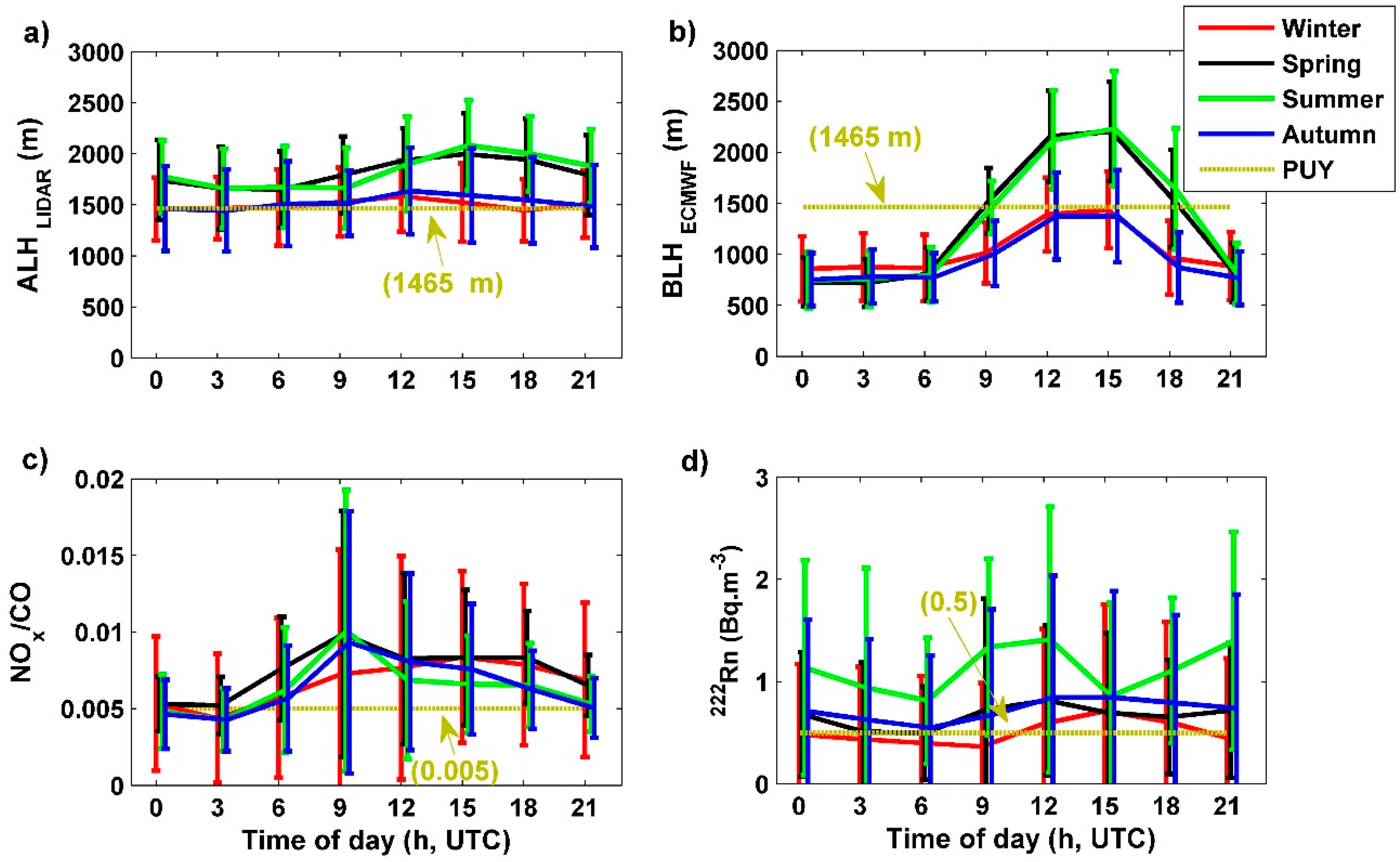
3.1.1. Comparison between the Aerosol Layer Height from LIDAR Profiles and Boundary Layer Height Simulated with ECMWF

Figure 2a shows the 3-h average diurnal variation of the ALH retrieved from the LIDAR profiles (ALH_LIDAR) for the four seasons separately (Winter: 1 January to 19 March, Spring: 20 March to 19 June, Summer: 20 June to 21 September, and Autumn: 22 September to 21 December) using data from 2015. The ALH_LIDAR does not show strong variations with the time of the day. The maximum of the ALH_LIDAR is reached during summer and spring (average 2000 m a.s.l., green and black) while in winter and autumn (red and blue), the average ALH_LIDAR never exceeds 1600 m. Lowest ALH_LIDAR are observed during night time, before 9 UTC, when the WCT most likely retrieves the height of the RL. These typical ALH diurnal and seasonal variations are similar to the ones previously reported for the PUY station (Figure 2 in Chauvigné et al. (2016) [36]) and for the Leipzig station (Figures 7, 9 and 17 in Baars et al. (2008) [13]). The LIDAR is located approximately 16 km to the east of the PUY station, that is, downwind of the North-South mountain chain for the western prevailing winds. It is likely that there is a deformation of the upwind atmospheric structure due to the obstacle that the mountain chain represents and, hence, we expect that the ALH retrieved by the LIDAR is slightly increased compared to the surrounding flat and low altitude areas.

BLH_ECMWF varies between 700 m a.s.l. at night in winter and 2200 m a.s.l. during the day in summer (Figure 2b). The model predicts that the PUY station is in the BL during the day (between 9 and 18 UTC) in summer and spring, with 3-h averaged BLH_ECMWF reaching a maximum of 2200 m a.s.l. In contrast, the model shows that the site is generally above the BL at all times during winter and autumn, and therefore considered to be in the FT. These results are in agreement with the study performed by Venzac et al. (2009) [14] who reported that the PUY station was in the BL during the daytime during the warm seasons (spring and summer) and in the FT during nighttime during the cold seasons (autumn and winter). The ECMWF model is not taking into account the forced convection on the mountain chain. Hence, we expect that the model underpredicts the BLH above the grid square.

Significant differences are observed between ALH_LIDAR and BLH_ECMWF during nighttime (Figure 2a,b). This is related to the fact that the LIDAR retrieves RLH, while BLH_ECMWF instead corresponds to the height of the shallower stable nocturnal BL. On the contrary, ALH_LIDAR can be compared to the BLH_ECMWF over the daytime period (9 UTC-18 UTC), when the AL can be assimilated to the convective BL. As evidenced in Figure 3, the ALH_LIDAR and BLH_ECMWF correlate and agree well with each other (correlation coefficient Pr = 0.6 and linear regression slope 0.78). The value of the slope below 1 either indicates an overestimation of the ALH_LIDAR or an underestimation of the BLH_ECMWF. As mentioned above, the overestimation of the ALH_LIDAR could be due to the deformation of the upwind atmospheric structure between CZ and PUY stations. Indeed, the ECMWF model spatial resolution does not take into account local scale dynamical processes around the PUY mountain chain (due to a flattening effect over the surface mode grid).

In order to assess if the PUY station is within the BL/AL or in the FT, the real forced convection from the local topography needs to be taken into account. We calculate the splitting height (SH) for both WCT and ECMWF methods, which corresponds to the height below which an air mass encountering an obstacle is going around it, and above which the air mass is overpassing it. Details of the method for calculating SH is described in Etling, (1989) [49], (Equation (3)).

SH = H (1 − Fr)

(3)

H is the height difference between the PUY station and the foot of the mountain and Fr is the Froude number [14,49]. When ALH/BLH are higher than the altitude of PUY, the station is always considered to be in the BL/AL. This is especially the case for unstable conditions (Fr > 1) when the BLH always reaches the PUY station after the air mass encounters the obstacle. For stable conditions (Fr < 1), two different situations are identified depending on SH. If the BLH/ALH is lower than SH, the stream will drift away from the obstacle, and the station will be in free tropospheric conditions. In contrast, for a BLH/ALH higher than SH, the air mass will be uplifted along the mountain slope, and the station will, hence, lay in the BL/AL (

Table 1. The classification of the air mass type (BL/AL or FT) sampled at the PUY station as a function of BLH/ALH, and Splitting Height (SH).

	Comparison of PUY Altitude, ALH/BLH and SH	PUY Conditions
Unstable Conditions	BLH/ALH > PUY	BL/AL
Stable Conditions	BLH/ALH > PUY	BL/AL
	BLH/ALH < PUY and BLH/ALH > SH	BL/AL
	BLH/ALH < PUY and BLH/ALH < SH	FT

). SH data was calculated every three hours for 2015.

3.1.2. NO_x/CO

NO_y/CO is an indicator of the “photochemical age” of an air mass that can be used to identify fresh pollution transported to high altitude sites from lower atmospheric layers [3,10]. Higher values of NO_y/CO represent fresh pollution, while lower values correspond to regional air masses. Hence, this ratio usually shows lower values in the FT than in the AL [3]. NO_y is defined as the sum of NO_x and its atmospheric oxidation products (that is, NO_z). In absence of NO_y measurements at PUY in 2015, we used NO_x data, since a good agreement between NO_y and NO_x is observed at this site based on measurements conducted in 2012 (Pr = 0.93 and slope = 1.11, Figure A2). We, therefore, consider that at the PUY, the NO_x measurements are a relatively good indicator of aged air masses. However, we are aware that NO_x measurements can often be influenced by more local emissions than NO_y, and care should be taken when interpreting these measurements.

For all seasons, we observe a clear diurnal variation with low values at night and high values during the day (Figure 2c). During daytime, an average NO_x/CO maximum of 0.01 was observed for spring, summer, and autumn, at 9 UTC. For winter, a maximum of 0.08 was reported at 18 UTC.

In order to determine whether NO_x/CO is a good indicator for segregating between AL and FT conditions, we investigated the linear regression between NO_x/CO and the BLH_ECMWF. We found that both criteria are correlated at the 95% significance level (Pr = 0.54) with the following equation determined over the one-year dataset:

$${\mathrm{BLH}}_{\mathrm{ECMWF}}=1204+1.3\times \left(\frac{1}{{\mathrm{NO}}_{\mathrm{x}}/\mathrm{CO}}\right)$$

(4)

This equation allowed us to determine a threshold value of NO_x/CO = 0.005 above which the PUY station is considered to be in the FT (that is, for BLH_ECMWF > 1465 m).

However, we observe that the diurnal amplitude of the NO_x/CO ratio varies according to the season (Figure 2c). As a consequence, using a yearly threshold, the site is considered to be in the AL during the day (between 6 and 21 UTC) and in the FT in the night (from 21 to 6 UTC) for all seasons.

3.1.3. Radon-222 (²²²Rn)

The last technique to evaluate AL/FT conditions is based on the level of ²²²Rn measured at the PUY station. ²²²Rn is naturally emitted from the land surface at a relatively constant rate [50,51]. Since ²²²Rn is naturally emitted from land surfaces, it is often used as a mean to determine the level of contact of the air mass to the land surface. Hence, the lower the value of ²²²Rn, the less contact the air mass has had with the AL. This criterion was recently used by Griffiths et al. (2014) [11] and Herrmann et al. (2015) [3] to study vertical mixing, based on sites at different altitudes [52] or on vertical profiles from aircraft [53,54,55]. It has also been used for the estimation of local to regional surface emissions of trace gases [56].

As shown in Figure 2d, the ²²²Rn concentration does not show strong seasonal variations at PUY, with the exception for summer. As expected, the maximum values of the ²²²Rn concentration are reached during summer (average 1.41 Bq·m⁻³), especially during daytime. This is likely caused by the increased vertical mixing of air masses during the summer transported to the PUY site. In winter, spring, and autumn, the average ²²²Rn concentrations never exceed 0.85 Bq·m⁻³. This can be a result of low vertical mixing height as observed from the LIDAR and ECMWF data, but also to a high fraction of air masses coming from the marine sectors (hence, naturally containing lower levels of ²²²Rn within the BL).

In order to proceed with the identification of AL/FT air masses based on ²²²Rn measurements, we followed the methodology introduced by Herrmann et al. (2015) [3] for the JFJ site, which is based on the relationship between the ²²²Rn levels and the number concentration of particles larger than 90 nm (N₉₀). As illustrated in Figure 4a, in a similar way as was done by Herrmann et al. (2015) [3], we first investigated the variations of N₉₀ as a function of the air mass residence time in the FT since last BL contact. As previously reported for the JFJ, we observed decreasing exponential trend of N₉₀ with time since the last BL contact, but the parameters of the fit are, however, different from those obtained for the JFJ. Specifically, the threshold value below which N₉₀ does not further decrease, that is, indicating FT background concentrations, is around 151 cm⁻³ at PUY, being almost 4 times higher than at JFJ (40 cm⁻³). This is likely to be explained by a higher proximity to the BL/FT inversion when the PUY station is in the FT, compared to when the JFJ is in the FT. Indeed, Chauvigné et al. (2016) [36] pointed out that the aerosol concentrations are not homogeneously distributed over the vertical column within the FT, with a negative aerosol concentration gradient with altitude also within the FT. Plotting N₉₀ as a function of the ²²²Rn level (Figure 4b) also shows a clear decreasing exponential trend that indicates that ²²²Rn is also a good indicator of the BL influence on the PUY station. Using a threshold of N₉₀ = 151 cm⁻³ on Figure 4b leads to a threshold of ²²²Rn = 0.5 Bq·m⁻³. This translates on Figure 2d to the PUY station being in the AL all the time during spring, summer, and autumn. For winter, the site would be in the FT before 10 am and after 8 pm.

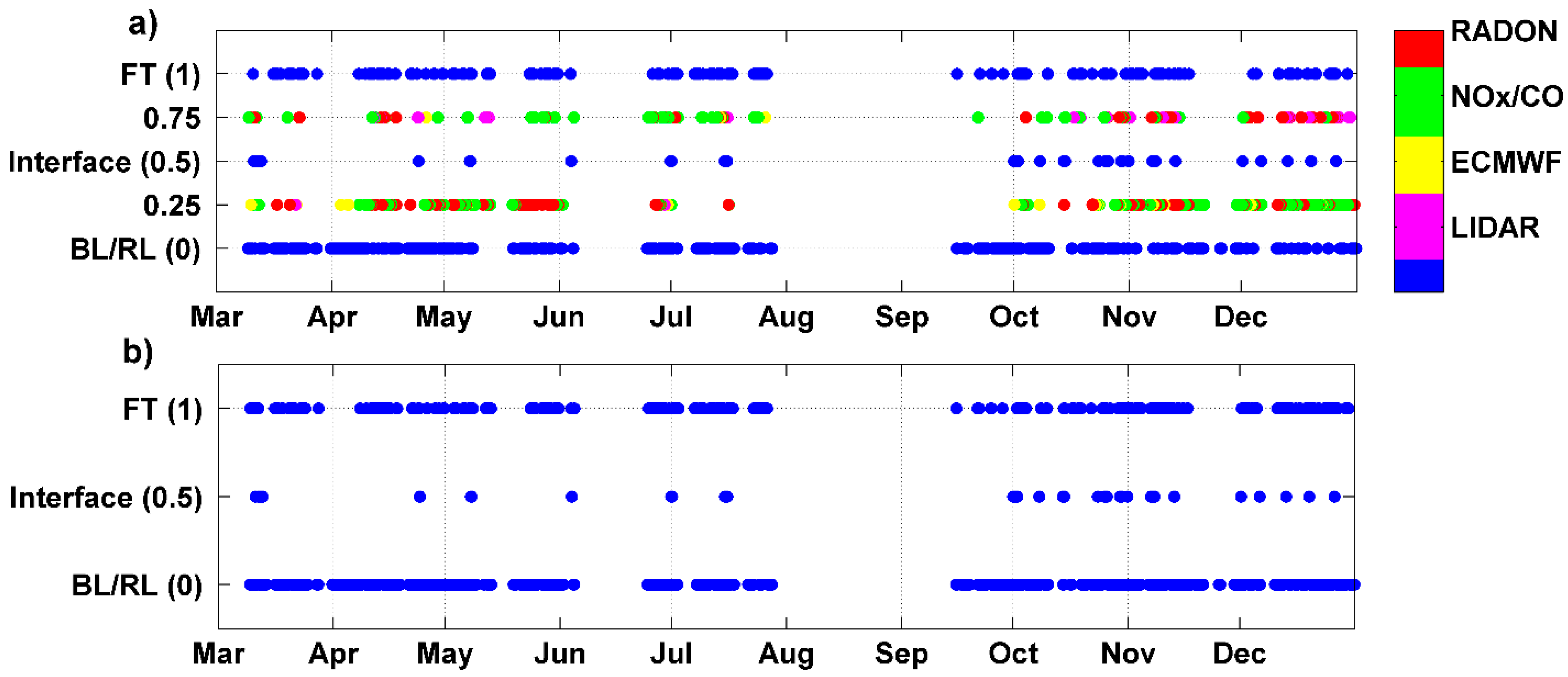
3.1.4. Comparison of the Four Criteria

Each of the four methods used to segregate whether the PUY station lies within the BL/AL or in the FT has specific criteria, based on the vertical profile of aerosols retrieved from LIDAR, on the “global method of Richardson” from the ECMWF model, the “photochemical age” of an air mass from NO_x/CO and the estimation of local to regional surface emissions of trace gases from ²²²Rn.

During daytime, the prediction of the BLH_ECMWF agrees relatively well with the ALH_LIDAR, but it should be noted that some uncertainties can be associated with these simulations due to forced convection and their horizontal distance from the site, as is discussed in Section 3.1.1 and shown in Figure 3 above. The NO_x/CO tracer would agree best with the prediction of the ECMWF in the sense that the diurnal variations of this indicator are clear between night and day, even though the seasonal variation is not very evident. It may be that these two criteria agree because NO_x/CO values are decreased in the residual layer compared to the daytime BL. The ²²²Rn tracer predicts that the site is in the BL with a similar trend than the ALH_LIDAR: the site is measured to be influenced by the BL most of the time except during winter and at night. Hence, ²²²Rn would be more sensitive to the presence of the residual layer at night than the NO_x/CO indicator. However, using a single set of measurements such as NO_x/CO, WCT from LIDAR, ECMWF, or ²²²Rn was not sufficient to classify air masses in the FT/(BL/AL) at the PUY station.

As all four criteria may have their own bias, a combined classification of these four criteria is proposed in order to increase the robustness of our methodology to determine if the PUY station is in the FT/(BL/AL).

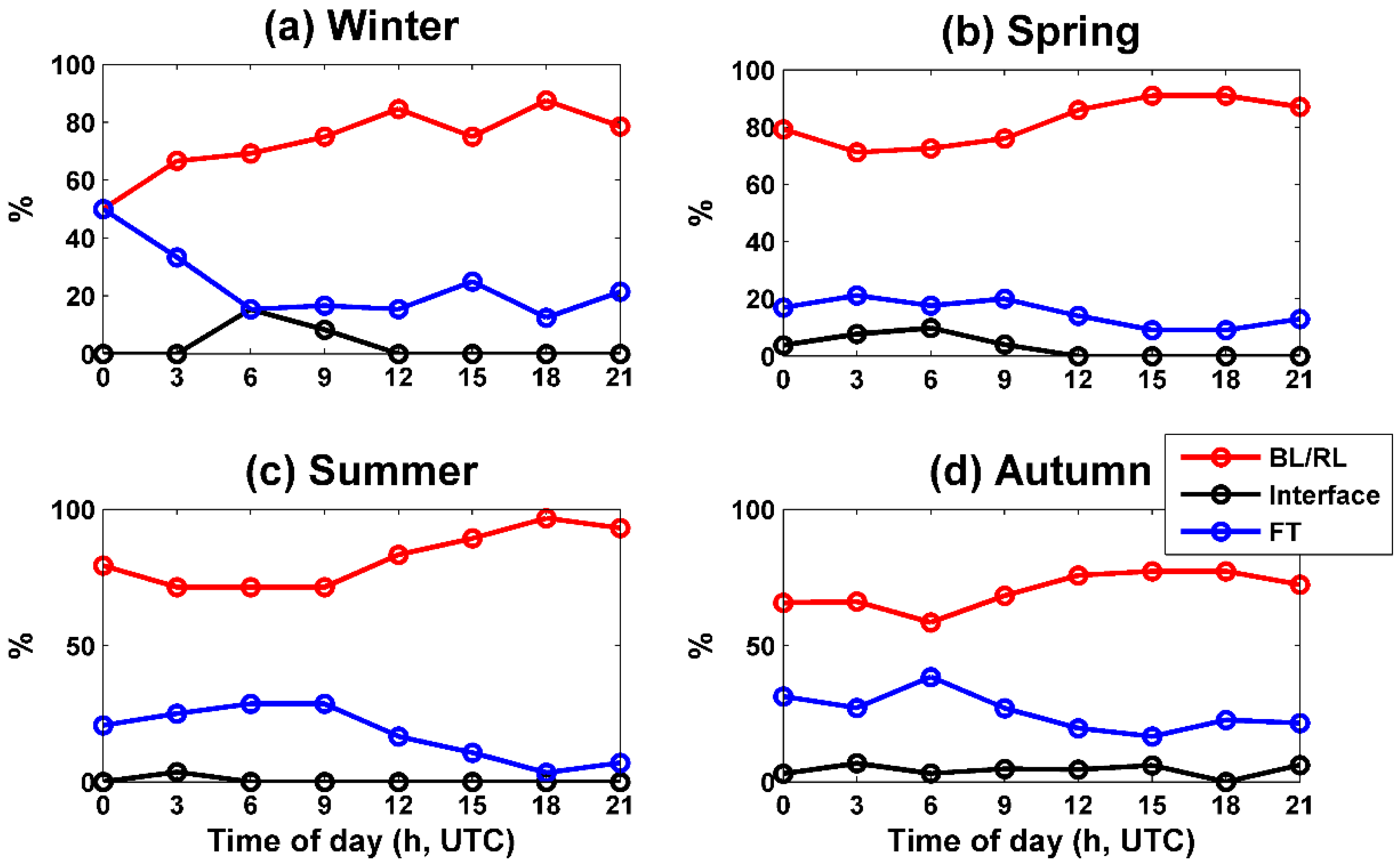
3.1.5. Classification of Air Masses by Combining Four Criteria

Venzac et al. (2009) [14] previously used temperature, relative humidity and the ECMWF model to separate BL and free tropospheric air masses at the PUY station. In this work, we present a more robust classification of air masses using a combination of four criteria (Figure 5a).

As mentioned above, WCT from LIDAR, NO_x/CO, and ²²²Rn retrieve the ALH while the ECMWF retrieves the BLH. However, AL corresponds to the BL during the daytime and RL during nighttime. For the simplicity of this work, we use the terminology BL/RL for BL, AL, and RL altogether. Thus, this section aims at using all available criteria to classify air masses sampled at the PUY station as those from the FT/(BL/RL).

Figure 5a shows the average classification of the measured air masses as FT/(BL/RL) at the PUY station. In order to average the four classification criteria, we use a specific labeling. When a measurement criterion classifies the air mass at the PUY station as FT, the corresponding date is labeled “1”, when it is classified as BL/RL air mass, the corresponding date is labeled “0”. Hence, when all four criteria give the air mass as FT, the average classification is “1”, while only three criteria out of four classify the air mass as FT, the average classification is “0.75”. Similarly, when all four criteria give the air mass as BL/RL, the average classification is “0”. Additionally, when two criteria of four go wrong for classifying the air mass as FT or BL/RL, the average classification is “0.5” which corresponds to the interface mode, while only one criteria out of four are classifying the air mass as BL/RL, the average classification is “0.25”. Colors in the figure correspond to the one criteria that differs from the other three. We observe that the WCT criteria did not identify FT air masses in the winter (violet color in 0.75). For classifications of BL/RL conditions, disagreements between the four methods were largely related to either NO_x/CO or ²²²Rn (green and red color, respectively in 0.25 (Figure 5)). For the tracer NO_x/CO, it is possible that this tracer is more representative of aged regional emissions as reported by Freney et al. (2011) [29]. ²²²Rn levels can also be influenced by the changes in air mass at PUY station. Indeed, for a given BLH, an oceanic air mass will have lower levels than a terrestrial air mass. Hence, we believe that ²²²Rn is the less reliable tracer of FT air masses for our site. This analysis also highlights that at the PUY station, radon and NO_x/CO overestimate when the PUY station is in the BL/AL than the other methods. ECMWF is also not adequate for the estimation of FT/BL conditions at night time, retrieving the stable nocturnal BL and not considering the residual nocturnal layer. By combining four criteria for the determination of FT or BL/RL conditions, we provide a more robust method. As a consequence, we chose to classify the station in FT air masses when 3 of the 4 criteria identify FT air masses (0.75) and classify the station in BL/RL air masses when the majority of methods identified BL/RL air masses (0.25). When only two out of four methods disagree with the others (0.5), the air mass is classified at the interface (Figure 5b).

At the PUY station, using a combination of these four criteria for assessing if the site is in free tropospheric conditions, we determine that the site is in the FT for 20% of the time as a yearly average, over 25% during winter and below 17% during summer. At the JFJ, Herrmann et al. (2015) [3] compared three criteria for assessing if the site lies in free tropospheric condition, and found FT prevalence for 39% of the time as a yearly average, with over 60% during winter and below 20% during summer. Chauvigné et al. (2018) [57], also reports time spent in the FT for the Chacaltaya (CHC) (5240 m a.s.l, Bolivia) site, and found FT prevalence for 45% of the time as a yearly average, with no marked seasonal variations. The difference between the PUY and these sites is probably that the PUY is at a lower altitude, but also because the configuration of the topography is different (North-South orientated single mountain chain) [58].

For the four seasons, the percentage of time that the site is in the BL/RL (red) increases during the day (between 9 and 18 UTC) to reach a maximum at 18 UTC, and decrease during the night (after 18 UTC) to reach a minimum at 00 h for winter, at 3 UTC for spring and summer, and at 6 UTC for autumn (Figure 6). On the contrary, this percentage in FT (blue) decreases during the day (between 9 and 18 UTC) to reach a minimum at 18 UTC for winter spring and summer, and at 15 UTC for autumn. During the night the percentage of FT air masses at the site reaches a maximum at 00 h for winter, at 3 UTC for spring, and at 6 UTC for summer and autumn.

Air masses are classified at the interface between the BL/RL and the FT (black), at a higher frequency at night/early morning than during the late evening, and higher during winter than during summer. Between 3 and 12 UTC, this percentage reaches a maximum of 15.5% and 10% at 6 UTC respectively for winter and spring. The high percentage at the interface is related to the diurnal variation of the BLH which reaches the PUY station at around 6 UTC.

3.2. Comparisons of the Free Troposphere and Boundary Layer Aerosol Properties

In this section, we use the classification proposed by the combination of the four criteria of FT/(BL/RL) segregation in order to investigate the differences of thermodynamical variables and aerosol properties when sampled in the BL/RL or in the FT at the PUY station. The values obtained for all criteria when the PUY station is at the interface between both layers represent a smaller database that is not statistically relevant and will not be discussed here (Table A1).

In order to assess whether the different parameters show statistically significant differences in FT/(BL/RL), the Wilcoxon–Mann–Whitney test [59] was applied to the median values (Temperature (T), Relative Humidity (RH), Pressure (P), Black Carbon (BC), and for the nucleation (Nuc), Aitken (Ait), accumulation (Acc) and coarse (Coa) aerosol particles size mode concentrations) (Figure 7). This nonparametric test evaluates the difference in medians between two similarly shaped populations. This test showed that the FT/(BL/RL) difference was significant for some parameters (for example, T, RH, and P), however, for certain parameters during certain seasons (for example, the BC and Acc mode particles in summer and for Nuc mode particles during all seasons) no differences between BL/RL and FT properties were detected.

At first, the meteorological parameters (T, RH, and P) were characterized in the FT and in BL/RL air masses (Figure 8a–c). As expected higher median RH concentrations were found in BL/RL conditions for all seasons compared to FT conditions, this difference is shown to be significant by the Wilcoxon–Mann–Whitney test (Figure 7). The higher RH in BL/RL conditions at the PUY station is the result of sources of humidity from the surface in the BL/RL. Higher median T and P were measured in FT conditions compared to BL/RL conditions for all seasons (except in winter for P), the significance being confirmed by the Wilcoxon–Mann–Whitney test (Figure 7). Higher pressures in the FT than in the BL/RL could be related to anticyclone conditions, which decrease the BLH [60]. Higher temperatures in the FT than in the BL/RL may be explained by the fact that the PUY station is situated in the lower part of the FT in which the temperature increases over a limited altitude range (temperature inversion starting at the very lower part of the FT) [61].

Figure 9a shows, for different seasons, the Black Carbon (BC) concentration when the PUY is in the FT or BL/RL. The Wilcoxon–Mann–Whitney test presented in Figure 7, shows that for winter, spring and autumn seasons, the null hypothesis that the two sets have equal medians was dismissed with a threshold of 5% (black square), while in summer the null hypothesis cannot be dismissed (transparent square). Hence it appears that in summer, there is no marked distinction between the median BC concentration in the FT and the median BC concentration in the BL/RL. However, we observe a stronger variability in the BC in the BL/RL than in the FT. This variation is likely due to the diurnal cycle of sources in this layer. In winter and autumn, the median BC concentration is significantly higher in the BL/RL compared to the FT. This is expected as sources of BC are mainly from surface emissions. In spring, we observe an unusual trend with BC concentrations significantly higher in the FT than in the BL/RL.

The high concentrations of BC in the BL/RL for winter and autumn are thought to be a result of higher contributions of local sources of combustion linked to conventional heating devices often observed during this time of the year [62]. This combined with lower BL heights results in an accumulation of these particle concentrations during the cold seasons. In spring and summer, transport of the materials from BL/RL to FT efficiently occurs by active convection, and the FT air masses are more impacted by intrusions of BL/RL air. The stronger BC concentration in the FT during spring can be linked to BC originating from biomass burning occurring frequently during this season during the burning of vegetation in gardens, that is likely injecting biomass burning particles directly into the FT from strong heat convection transport from BL/RL to FT.

In addition, Figure 9b represents median aerosol size distributions (10–650 nm) for the four seasons, in the BL/RL and FT, and highlights the various shapes observed in the different conditions. In order to further investigate the seasonal variation of the aerosol spectrum properties in both layers, we used four aerosol modes: nucleation (10 nm to 20 nm), Aitken (40 nm to 80 nm), accumulation (100 nm to 300 nm), and coarse (1 µm to 18 µm) modes (Figure 9c–f). During the winter and autumn months, the median Aitken and accumulation mode aerosol concentrations are significantly higher in the BL/RL, compared to the FT (Figure 9d,e). In spring (for the accumulation mode) and spring and summer (for the Aitken mode), we observe the opposite, with higher concentrations in the FT than in the BL/RL. In summer, the median accumulation mode particle concentration is comparable in the FT and in the BL/RL.

For nucleation mode particles (10–20 nm) (Figure 9c), there are no significant differences in median values in the FT and in the BL/RL for all seasons. The lack of difference between nucleation mode particles in the BL/RL and in the FT would suggest that there is an additional source of nucleation mode particles in the FT compared to the primary emissions traced by the accumulation mode particles during winter and autumn. This was already observed by Tröstl et al. (2016) [63] at the JFJ site who reports that the nucleation mode particles occur within air masses that have been transported over long-range distances into the FT.

Additionally, these particles show the highest concentrations during summer (N_{nuc, FT} = 489 cm⁻³; N_{nuc, BL/RL} = 512 cm⁻³) (

Table 2. The mean concentration of the Nucleation, Aitken, and Accumulation mode particles for the four seasons.

Particle Mode	Season	N (cm−3)
		FT	BL/RL
Nucleation	Winter	190	254
	Spring	490	504
	Summer	489	512
	Autumn	374	312
Aitken	Winter	346	514
	Spring	1211	714
	Summer	1119	823
	Autumn	367	419
Accumulation	Winter	290	530
	Spring	630	470
	Summer	560	570
	Autumn	220	385

). This is in agreement with Venzac et al. (2009) [14] at the same site, who reports highest concentrations of nucleation mode particles during summer [14]). Boulon et al. (2011) [27] reports the highest new particle formation frequency during spring and autumn, but the intensity of the new particle formation events (in term of nucleation rate and further growth) is the highest during summer.

The accumulation mode particle concentrations have a similar behavior to the BC concentrations previously discussed, and we assume that they have similar sources for winter and autumn. Higher concentrations of the Aitken mode particles during springtime may be partly due to the growth of nucleation mode particles that were observed to occur more frequently during spring [24,26] and preferentially at higher altitudes [27], as also witnessed by higher concentrations during the spring season for the present dataset, and partly due to a contribution from biomass burning aerosols due to the active convection transport from BL/RL to FT. During summer, the difference between concentrations in the FT and in the BL/RL is less marked than in Spring, which may be due to the less frequent nucleation frequency [27,64] and the less biomass burning events than in spring.

For both accumulation and Aitken mode concentrations, we clearly see that spring and summer (N_{accumulation, spring, FT} = 630 cm⁻³; N_{accumulation, spring, BL/RL} = 470 cm⁻³; N_{aitken, spring, FT} = 1211 cm⁻³; N_{aitken, spring, BL/RL} = 714 cm⁻³ and N_{accumulation, summer, FT} = 560 cm⁻³; N_{accumulation, summer, BL/RL} = 570 cm⁻³; N_{aitken, summer, FT} = 1119 cm⁻³; N_{aitken, summer, BL/RL} = 823 cm⁻³) show the highest mean particle concentrations in both the FT and the BL/RL (Table 2). This is in agreement with that of Venzac et al. (2009) [14] and Herrmann et al. (2015) [3] during the summer season.

In our study, the observed concentrations are slightly higher then what was found by Venzac et al. (2009) [14]. This would confirm the tendency observed by Venzac et al. (2009) [14] of the aerosol concentration increasing over the 6 years of data but would need a careful trend analysis which is beyond the scope of the present study.

For coarse mode particles, no data is available for winter and autumn, and the Wilcoxon–Mann–Whitney test is not significant for spring (medians are equal for FT and BL/RL) (Figure 9f). However, for summer, high median concentrations of the coarse mode particles were measured in FT conditions, compared to the BL/RL conditions. This difference is likely due to a more efficient long-range transport of dust and marine aerosols at high altitudes than at lower altitudes. Bourcier et al. (2012) [30] reported higher concentrations of Cesium (Cs) associated to dust particles at PUY, than at the lower altitude of CZ, but the difference was mostly found during winter. The authors hypothesized that during winter, large particles are transported with a higher efficiency at high altitudes due to stronger winds. The variability of the coarse mode particle concentration is higher during the BL/RL conditions compared to FT conditions presumably due to the sporadic character of sources of large primary particles in the BL/RL.

The next step of our analysis is to investigate the variability of aerosol properties within the lower FT and the possible causes for this variability.

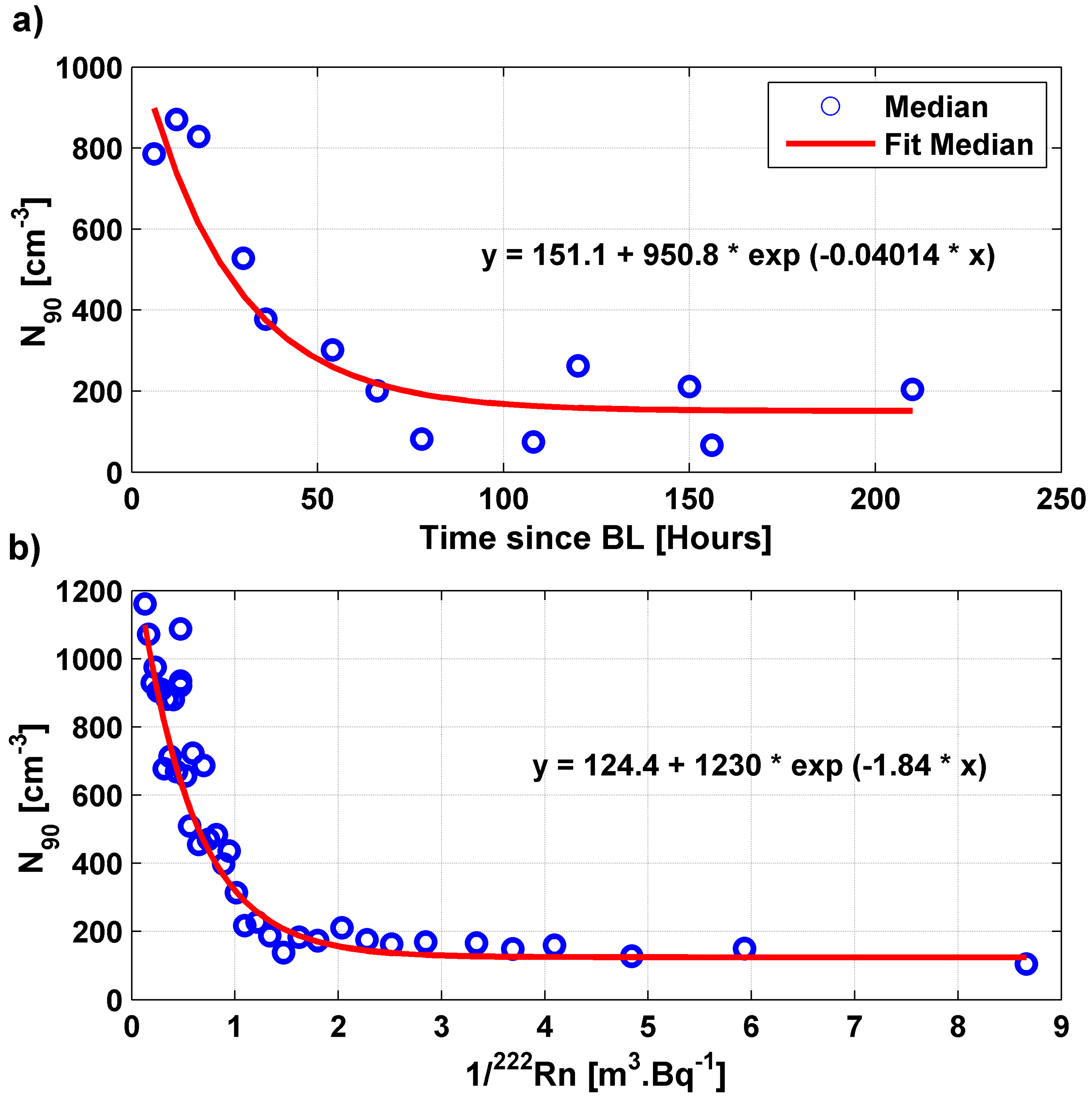
3.3. Aerosol Properties in the Lower Free Troposphere as a Function of Air Mass Type and Age

Our analysis of the air mass back-trajectory history relative to the latest contact with the BL over the 204-h prior sampling showed that air masses aerosol properties (for example, N₉₀) do not change for BL-contact-free times larger than 75 h (Figure 4a). In the following section, we investigate the change of aerosol particles within the lower free troposphere during the last 75 h prior to sampling.

Figure 10 presents the segregation of FT air masses as a function of the time they spent in the FT since their last contact with the BL/RL before reaching the PUY station. The BLH parameter of ERA-Interim ECMWF is interpolated spatially and temporally and compared with the altitude of each path point to determine the last contact with the BL. This analysis was done using LACYTRAJ, for the four seasons. Most noticeably, the vast majority (over 80%) of winter and autumn air masses did not have any contact with the BL/RL for at least the last 75 h before being sampled at PUY. This explains why certain aerosol concentrations are low in the FT during these seasons. For summer and spring, the large majority (60%) of air masses were in contact with the BL/RL in the last 15 h prior to measurement (Figure 10). Therefore, certain aerosol concentrations are high in the FT during these seasons. We hence assume that aerosol properties measured in these air masses during summer and spring are more representative of BL/RL than the unperturbed FT. Using this information, we focus the remaining discussion on aerosol properties measured during winter and autumn assuming that they are representative of the unperturbed FT and we can, therefore, study their characteristics as a function of the air mass origin.

LACYTRAJ has also been used to provide a classification of five possible sources, from Oceanic, Mediterranean, continental, northerly, or local (Figure 11), similar to Asmi et al. (2012) [28] and Rose et al. (2015a) [24] (details of the classification are shown in Figure A3). This classification is based on the location of the last interaction between the air mass and the BL. Therefore, the locations of the last contact with BL are essential. During the winter season, air masses are mainly of Mediterranean (34%) and Atlantic (29%) origins, and a smaller fraction of them are either local (15%), continental (14%), or Atlantic modified (8%) (Figure 11). In autumn, air masses are mostly of Mediterranean (39%) and Atlantic (48%) origins, and a small fraction is of a continental origin (12%) (Figure 11).

In the following section we compare aerosol properties in the three types of air masses (Atlantic, Mediterranean, and Continental) observed during both seasons (winter and autumn) (Figure 12).

Higher nucleation mode concentrations are measured when the PUY station is exposed to aged (>75 h) Atlantic and Mediterranean air masses than when exposed to continental air masses (Figure 12). We can hypothesize that these high concentrations of nucleation mode aerosols are formed at the PUY from marine precursor sources that have been transported from the Mediterranean sea and from the Atlantic ocean [24,65], or that the condensational sink associated to the Atlantic and Mediterranean air mass types are lower compared to continental air masses containing larger concentrations of accumulation mode particles. Bianchi et al. (2016) [66] and Tröstl et al. (2016) [63] show also that nucleation in the FT is favored after a certain time lapse has passed after the last contact with the BL/RL.

In aged air masses, the high concentrations of the Aitken and accumulation mode particles coincide with the high concentrations of BC, originated from continental air masses. These high BC, Aitken, and accumulation concentrations can, thus, partly be due to biomass burning emissions. Another source of these high concentrations of Aitken mode particles is the growth of nucleation mode particles originated from the Atlantic and Mediterranean air masses. Within aged air masses, coarse mode aerosol concentrations are also higher in Mediterranean and Atlantic air masses compared to continental air masses, likely a result of transported sea salt and dust particles.

Overall, we observe that even after more than 75 h with no contact with the BL/RL, FT aerosols preserve properties that are specific to their source region. To the author’s knowledge, this is the first report of these observations from in situ measurements.

4. Conclusions

A one-year dataset of multiple measurements acquired at the PUY station has been used in this work to determine the specific physical characteristics of FT aerosols and hence of their sources and transport pathways from the BL.

In order to achieve this goal, a combination of four criteria was used to identify whether the PUY station lies within the FT or within the BL. BLH was determined using two independent methods, firstly the ECMWF model, using the “global method of Richardson” to calculate the BLH_ECMWF, and secondly, the WCT method to calculate the ALH_WCT from LIDAR measurements. In addition, NO_x/CO and radon-222 tracers were used to determine the degree of influence from the AL_NOx/CO and AL_Rn, respectively. Using these tracers, we observe that the PUY station is considered to be in the FT up to 50% during the winter months.

For most of the time and aerosol property, higher concentrations are found in the BL compared to FT, as expected from larger sources originating from the surface. However, higher BC, accumulation, and Aitken modes median concentrations are observed in FT conditions compared to BL during spring. This might be linked to biomass burning from vegetation in gardens that inject aerosols directly to the FT from active convection transport. Another source of these high concentrations of Aitken mode particles is the growth of nucleation mode particles. In general, for these nucleation mode particles, there is no significant difference in the median values measured in the FT and in the BL/RL for all seasons. This suggests that there is an additional source of precursors to the formation of new particles at the PUY station. These additional sources likely originate from aged Atlantic or Mediterranean air masses. Higher median concentrations and higher variability of the coarse mode particles are also found in FT conditions during summer is a result of increased contribution from Mediterranean and Atlantic air masses, bringing dust and marine aerosol at higher altitudes. Finally, even after more than 75 h without any contact with the BL/RL, FT aerosols preserve properties specific to their air mass type/origin. However, as expected, these differences are less distinct in aged FT air masses (>75 h) than in recent FT air masses (>15 h).

This work introduces a robust method to establish when a site is in the FT or in the BL/RL. Using this method, we were able to identify typical physical properties of different air mass sources in both the BL/RL and in the FT. This method has been applied to the PUY site, which is at the frontier of the BL and the FT, where the majority of exchanges and interactions occur, making it a unique area to study these exchanges. The method of differentiating between BL/RL and FT used in this work can be applied to future studies at altitude sites, providing a real-time estimate of FT air mass sampling. These aerosol properties (size, number concentration, and so forth) can subsequently be used for comparison with different aerosol transport models outputs.

References

1. Stocker, T.F.; Qin, D.; Plattner, G.-K.; Tignor, M.; Allen, S.K.; Boschung, J.; Nauels, A.; Xia, Y.; Bex, V.; Midgley, P.M. IPCC, 2013: Climate Change 2013: The Physical Science Basis; Contribution of Working Group I to the Fifth Assessment Report of the Intergovernmental Panel on Climate Change; Cambridge University Press: Cambridge, UK; New York, NY, USA, 2013; p. 1535. [Google Scholar]
2. Stull, R.B. An Introduction to Boundary Layer Meteorology; Springer: Dordrecht, The Netherlands, 1988. [Google Scholar]
3. Herrmann, E.; Weingartner, E.; Henne, S.; Vuilleumier, L.; Bukowiecki, N.; Steinbacher, M.; Conen, F.; Collaud Coen, M.; Hammer, E.; Jurányi, Z.; et al. Analysis of long-term aerosol size distribution data from Jungfraujoch with emphasis on free tropospheric conditions, cloud influence, and air mass transport. J. Geophys. Res. Atmos. 2015, 120, 9459–9480. [Google Scholar] [CrossRef]
4. De Wekker, S.F.J.; Kossmann, M. Convective Boundary Layer Heights over Mountainous Terrain—A Review of Concepts. Front. Earth Sci. 2015, 3, 1–22. [Google Scholar] [CrossRef]
5. Holzworth, G.C. Estimates of Mean Maximum Mixing Depths in the Contiguous United States. Mon. Weather Rev. 1964, 92, 235–242. [Google Scholar] [CrossRef]
6. Holtslag, A.A.M.; De Bruijn, E.I.F.; Pan, H.-L. A High Resolution Air Mass Transformation Model for Short-Range Weather Forecasting. Mon. Weather Rev. 1990, 118, 1561–1575. [Google Scholar] [CrossRef] [Green Version]
7. Seibert, P.; Beyrich, F.; Gryning, S.-E.; Joffre, S.; Rasmussen, A.; Tercier, P. Review and intercomparison of operational methods for the determination of the mixing height. Atmos. Environ. 2000, 34, 1001–1027. [Google Scholar] [CrossRef]
8. Emeis, S.; Münkel, C.; Vogt, S.; Müller, W.J.; Schäfer, K. Atmospheric boundary-layer structure from simultaneous SODAR, RASS, and ceilometer measurements. Atmos. Environ. 2004, 38, 273–286. [Google Scholar] [CrossRef]
9. Wiegner, M.; Emeis, S.; Freudenthaler, V.; Heese, B.; Junkermann, W.; Münkel, C.; Schäfer, K.; Seefeldner, M.; Vogt, S. Mixing layer height over Munich, Germany: Variability and comparisons of different methodologies. J. Geophys. Res. Atmos. 2006, 111, D13201. [Google Scholar] [CrossRef]
10. Zellweger, C.; Forrer, J.; Hofer, P.; Nyeki, S.; Schwarzenbach, B.; Weingartner, E.; Ammann, M.; Baltensperger, U. Partitioning of reactive nitrogen (NOy) and dependence on meteorological conditions in the lower free troposphere. Atmos. Chem. Phys. 2003, 3, 779–796. [Google Scholar] [CrossRef]
11. Griffiths, A.D.; Conen, F.; Weingartner, E.; Zimmermann, L.; Chambers, S.D.; Williams, A.G. Surface-to-mountaintop transport characterised by radon observations at the Jungfraujoch. Atmos. Chem. Phys. 2014, 14, 12763–12779. [Google Scholar] [CrossRef] [Green Version]
12. Chambers, S.D.; Williams, A.G.; Conen, F.; Griffiths, A.D.; Reimann, S.; Steinbacher, M.; Krummel, P.B.; Steele, L.P.; van der Schoot, M.V. Towards a universal “baseline” characterisation of air masses for high-and low-altitude observing stations using Radon-222. Aerosol Air Qual. Res. 2016, 16, 885–899. [Google Scholar] [CrossRef]
13. Baars, H.; Ansmann, A.; Engelmann, R.; Althausen, D. Continuous monitoring of the boundary-layer top with lidar. Atmos. Chem. Phys. 2008, 8, 7281–7296. [Google Scholar] [CrossRef] [Green Version]
14. Venzac, H.; Sellegri, K.; Villani, P.; Picard, D.; Laj, P. Seasonal variation of aerosol size distributions in the free troposphere and residual layer at the puy de Dôme station, France. Atmos. Chem. Phys. 2009, 9, 1465–1478. [Google Scholar] [CrossRef] [Green Version]
15. Hov, Ø.; Flatøy, F. Convective Redistribution of Ozone and Oxides of Nitrogen in the Troposphere over Europe in Summer and Fall. J. Atmos. Chem. 1997, 28, 319–337. [Google Scholar] [CrossRef]
16. Moorthy, K.K.; Sreekanth, V.; Prakash Chaubey, J.; Gogoi, M.M.; Suresh Babu, S.; Kumar Kompalli, S.; Bagare, S.P.; Bhatt, B.C.; Gaur, V.K.; Prabhu, T.P.; et al. Fine and ultrafine particles at a near–free tropospheric environment over the high-altitude station Hanle in the Trans-Himalaya: New particle formation and size distribution. J. Geophys. Res. 2011, 116, D20212. [Google Scholar] [CrossRef]
17. Rose, C.; Boulon, J.; Hervo, M.; Holmgren, H.; Asmi, E.; Ramonet, M.; Laj, P.; Sellegri, K. Long-term observations of cluster ion concentration, sources and sinks in clear sky conditions at the high-altitude site of the Puy de Dôme, France. Atmos. Chem. Phys. 2013, 13, 11573–11594. [Google Scholar] [CrossRef] [Green Version]
18. Kompalli, S.K.; Babu, S.S.; Krishna Moorthy, K.; Gogoi, M.M.; Nair, V.S.; Chaubey, J.P. The formation and growth of ultrafine particles in two contrasting environments: A case study. Ann. Geophys. 2014, 32, 817–830. [Google Scholar] [CrossRef] [Green Version]
19. Freney, E.; Sellegri Karine, S.K.; Eija, A.; Clemence, R.; Aurelien, C.; Jean-Luc, B.; Aurelie, C.; Hervo Maxime, H.M.; Nadege, M.; Laeticia, B.; et al. Experimental Evidence of the Feeding of the Free Troposphere with Aerosol Particles from the Mixing Layer. Aerosol Air Qual. Res. 2016, 16, 702–716. [Google Scholar] [CrossRef] [Green Version]
20. Mckendry, I.G.; Hacker, J.P.; Stull, R.; Sakiyama, S.; Mignacca, D.; Reid, K. Long-range transport of Asian dust to the Lower Fraser Valley, British Columbia, Canada: Quantifying the radiative impacts of mineral dust (DUST). J. Geophys. Res. 2001, 106, 18361–18370. [Google Scholar] [CrossRef]
21. Timonen, H.; Wigder, N.; Jaffe, D. Influence of background particulate matter (PM) on urban air quality in the Pacific Northwest. J. Environ. Manag. 2013, 129, 333–340. [Google Scholar] [CrossRef] [PubMed]
22. Martin, S.T.; Hung, H.-M.; Park, R.J.; Jacob, D.J.; Spurr, R.J.D.; Chance, K.V.; Chin, V. Effects of the physical state of tropospheric ammonium-sulfate-nitrate particles on global aerosol direct radiative forcing. Atmos. Chem. Phys. 2004, 4, 183–214. [Google Scholar] [CrossRef] [Green Version]
23. Crumeyrolle, S.; Schwarzenboeck, A.; Sellegri, K.; Burkhart, J.F.; Stohl, A.; Gomes, L.; Quennehen, B.; Roberts, G.; Weigel, R.; Roger, J.C.; et al. Overview of aerosol properties associated with air masses sampled by the ATR-42 during the EUCAARI campaign (2008). Atmos. Chem. Phys. 2012, 12, 9451–9490. [Google Scholar] [CrossRef]
24. Rose, C.; Sellegri, K.; Freney, E.; Dupuy, R.; Colomb, A.; Pichon, J.-M.; Ribeiro, M.; Bourianne, T.; Burnet, F.; Schwarzenboeck, A. Airborne measurements of new particle formation in the free troposphere above the Mediterranean Sea during the HYMEX campaign. Atmos. Chem. Phys. 2015, 15, 10203–10218. [Google Scholar] [CrossRef] [Green Version]
25. Fröhlich, R.; Cubison, M.J.; Slowik, J.G.; Bukowiecki, N.; Canonaco, F.; Henne, S.; Herrmann, E.; Gysel, M.; Steinbacher, M.; Baltensperger, U.; et al. Fourteen months of on-line measurements of the non-refractory submicron aerosol at the Jungfraujoch (3580 m a.s.l.)—Chemical composition, origins and organic aerosol sources. Atmos. Chem. Phys. 2015, 15, 11373–11398. [Google Scholar] [CrossRef]
26. Venzac, H.; Sellegri, K.; Laj, P. Nucleation events detected at the high altitude site of the Puy de Dôme Research Station, France. Boreal Environ. Res. 2007, 12, 345–359. [Google Scholar]
27. Sellegri, K.; Hervo, M.; Picard, D.; Pichon, J.-M.; Fréville, P.; Laj, P. Investigation of nucleation events vertical extent: A long term study at two different altitude sites. Atmos. Chem. Phys. 2011, 11, 5625–5639. [Google Scholar]
28. Asmi, E.; Freney, E.; Hervo, M.; Picard, D.; Rose, C.; Colomb, A.; Sellegri, K. Aerosol cloud activation in summer and winter at puy-de-Dôme high altitude site in France. Atmos. Chem. Phys. 2012, 12, 11589–11607. [Google Scholar] [CrossRef] [Green Version]
29. Freney, E.J.; Sellegri, K.; Canonaco, F.; Boulon, J.; Hervo, M.; Weigel, R.; Pichon, J.M.; Colomb, A.; Prévôt, A.S.H.; Laj, P. Seasonal variations in aerosol particle composition at the puy-de-Dôme research station in France. Atmos. Chem. Phys. 2011, 11, 13047–13059. [Google Scholar] [CrossRef] [Green Version]
30. Bourcier, L.; Sellegri, K.; Chausse, P.; Pichon, J.M.; Laj, P. Seasonal variation of water-soluble inorganic components in aerosol size-segregated at the puy de Dôme station (1465 m a.s.l.), France. J. Atmos. Chem. 2012, 69, 47–66. [Google Scholar] [CrossRef]
31. Sellegri, K.; Laj, P.; Dupuy, R.; Legrand, M.; Preunkert, S.; Putaud, J.-P. Size-dependent scavenging efficiencies of multicomponent atmospheric aerosols in clouds. J. Geophys. Res. 2003, 108, AAC3.1–AAC3.15. [Google Scholar] [CrossRef]
32. Guyot, G.; Gourbeyre, C.; Febvre, G.; Shcherbakov, V.; Burnet, F.; Dupont, J.-C.; Sellegri, K.; Jourdan, O. Quantitative evaluation of seven optical sensors for cloud microphysical measurements at the Puy-de-Dôme Observatory, France. Atmos. Meas. Tech. 2015, 8, 4347–4367. [Google Scholar] [CrossRef] [Green Version]
33. Burkart, J.; Steiner, G.; Reischl, G.; Moshammer, H.; Neuberger, M.; Hitzenberger, R. Characterizing the performance of two optical particle counters (Grimm OPC1.108 and OPC1.109) under urban aerosol conditions. J. Aerosol Sci. 2010, 41, 953–962. [Google Scholar] [CrossRef] [PubMed]
34. Hervo, M.; Quennehen, B.; Kristiansen, N.I.; Boulon, J.; Stohl, A.; Fréville, P.; Pichon, J.-M.; Picard, D.; Labazuy, P.; Gouhier, M.; et al. Physical and optical properties of 2010 Eyjafjallajökull volcanic eruption aerosol: Ground-based, Lidar and airborne measurements in France. Atmos. Chem. Phys. 2012, 12, 1721–1736. [Google Scholar] [CrossRef] [Green Version]
35. Freville, P.; Montoux, N.; Baray, J.-L.; Chauvigné, A.; Réveret, F.; Hervo, M.; Dionisi, D.; Payen, G.; Sellegri, K. LIDAR Developments at Clermont-Ferrand—France for Atmospheric Observation. Sensors 2015, 15, 3041–3069. [Google Scholar] [CrossRef] [PubMed] [Green Version]
36. Chauvigné, A.; Sellegri, K.; Hervo, M.; Montoux, N.; Freville, P.; Goloub, P. Comparison of the aerosol optical properties and size distribution retrieved by sun photometer with in situ measurements at midlatitude. Atmos. Meas. Tech. 2016, 9, 4569–4585. [Google Scholar] [CrossRef] [Green Version]
37. Brooks, I.M. Finding boundary layer top: Application of a wavelet covariance transform to lidar backscatter profiles. J. Atmos. Ocean. Technol. 2003, 20, 1092–1105. [Google Scholar] [CrossRef]
38. Villani, P.; Picard, D.; Marchand, N.; Laj, P. Design and Validation of a 6-Volatility Tandem Differential Mobility Analyzer (VTDMA). Aerosol Sci. Technol. 2007, 41, 898–906. [Google Scholar] [CrossRef] [Green Version]
39. Jokinen, V.; Mäkelä, J.M. Closed-loop arrangement with critical orifice for DMA sheath/excess flow system. J. Aerosol Sci. 1997, 28, 643–648. [Google Scholar] [CrossRef]
40. Wiedensohler, A.; Birmili, W.; Nowak, A.; Sonntag, A.; Weinhold, K.; Merkel, M.; Wehner, B.; Tuch, T.; Pfeifer, S.; Fiebig, M.; et al. Mobility particle size spectrometers: Harmonization of technical standards and data structure to facilitate high quality long-term observations of atmospheric particle number size distributions. Atmos. Meas. Tech. 2012, 5, 657–685. [Google Scholar] [CrossRef] [Green Version]
41. Müller, T.; Henzing, J.S.; de Leeuw, G.; Wiedensohler, A.; Alastuey, A.; Angelov, H.; Bizjak, M.; Collaud Coen, M.; Engström, J.E.; Gruening, C.; et al. Characterization and intercomparison of aerosol absorption photometers: Result of two intercomparison workshops. Atmos. Meas. Tech. 2011, 4, 245–268. [Google Scholar] [CrossRef] [Green Version]
42. Petzold, A.; Schönlinner, M. Multi-angle absorption photometry—A new method for the measurement of aerosol light absorption and atmospheric black carbon. J. Aerosol Sci. 2004, 35, 421–441. [Google Scholar] [CrossRef]
43. Biraud, S.; Ciais, P.; Ramonet, M.; Simmonds, P.; Kazan, V.; Monfray, P.; O’Doherty, S.; Spain, T.G.; Jennings, S.G. European greenhouse gas emissions estimated from continuous atmospheric measurements and radon 222 at Mace Head, Ireland. J. Geophys. Res. Atmos. 2000, 105, 1351–1366. [Google Scholar] [CrossRef] [Green Version]
44. Polian, G.; Lambert, G.; Ardouin, B.; Jegou, A. Long-range transport of continental radon in subantarctic and antarctic areas. Tellus B 1986, 38, 178–189. [Google Scholar] [CrossRef]
45. Schmidt, M. Measurement and balancing anthropogenic greenhouse gases in Germany. Ph.D. Thesis, Univ. Heidelberg, Heidelberg, Germany, 1999. [Google Scholar]
46. Von Engeln, A.; Teixeira, J. A Planetary Boundary Layer Height Climatology Derived from ECMWF Reanalysis Data. J. Clim. 2013, 26, 6575–6590. [Google Scholar] [CrossRef]
47. Troen, I.B.; Mahrt, L. A simple model of the atmospheric boundary layer; sensitivity to surface evaporation. Bound.-Layer Meteorol. 1986, 37, 129–148. [Google Scholar] [CrossRef] [Green Version]
48. Clain, G.; Baray, J.L.; Delmas, R.; Keckhut, P.; Cammas, J.P. A lagrangian approach to analyse the tropospheric ozone climatology in the tropics: Climatology of stratosphere-troposphere exchange at Reunion Island. Atmos. Environ. 2010, 44, 968–975. [Google Scholar] [CrossRef]
49. Etling, D. On atmospheric vortex streets in the wake of large islands. Meteorol. Atmos. Phys. 1988, 41, 157–164. [Google Scholar] [CrossRef]
50. Szegvary, T.; Leuenberger, M.C.; Conen, F. Predicting terrestrial 222Rn flux using gamma dose rate as a proxy. Atmos. Chem. Phys. 2007, 7, 2789–2795. [Google Scholar] [CrossRef] [Green Version]
51. Zhang, K.; Feichter, J.; Kazil, J.; Wan, H.; Zhuo, W.; Griffiths, A.D.; Sartorius, H.; Zahorowski, W.; Ramonet, M.; Schmidt, M.; et al. Radon activity in the lower troposphere and its impact on ionization rate: A global estimate using different radon emissions. Atmos. Chem. Phys. 2011, 11, 7817–7838. [Google Scholar] [CrossRef] [Green Version]
52. Chevillard, A.; Ciais, P.; Karstens, U.; Heimann, M.; Schmidt, M.; Levin, I.; Jacob, D.; Podzun, R.; Kazan, V.; Sartorius, H.; et al. Transport of 222Rn using the regional model REMO: A detailed comparison with measurements over Europe. Tellus B 2002, 54, 850–871. [Google Scholar] [CrossRef]
53. Guedalia, D.; Lopez, A.; Fontan, J.; Birot, A. Aircraft Measurements of Rn-222, Aitken Nuclei and Small Ions up to 6 km. J. Appl. Meteorol. 1972, 11, 357–365. [Google Scholar] [CrossRef]
54. Lee, H.N.; Larsen, R.J. Vertical Diffusion in the Lower Atmosphere Using Aircraft Measurements of 222Rn. J. Appl. Meteorol. 1997, 36, 1262–1270. [Google Scholar] [CrossRef]
55. Williams, A.G.; Zahorowski, W.; Chambers, S.; Griffiths, A.; Hacker, J.M.; Element, A.; Werczynski, S. The Vertical Distribution of Radon in Clear and Cloudy Daytime Terrestrial Boundary Layers. J. Atmos. Sci. 2010, 68, 155–174. [Google Scholar] [CrossRef]
56. Van der Laan, S.; van der Laan-Luijkx, I.T.; Zimmermann, L.; Conen, F.; Leuenberger, M. Net CO2 surface emissions at Bern, Switzerland inferred from ambient observations of CO2, δ(O2/N2), and 222Rn using a customized radon tracer inversion. J. Geophys. Res. Atmos. 2014, 119, 2013JD020307. [Google Scholar] [CrossRef]
57. Chauvigné, A.; Marcos, A.; Aliaga, D.; Radovan, K.; Grisa, M.; Montoux, N.; Moreno, I.; Thomas, M.; Marco, P.; Sellegri, K.; et al. Aerosol Optical Properties and Radiative forcing in the Andes Cordilliera based on measurements at the Chacaltaya observatory, Bolivia (5240 m a.s.l.). To be Submitt. 2018. [Google Scholar]
58. Collaud Coen, M.; Andrews, E.; Aliaga, D.; Andrade, M.; Angelov, H.; Bukowiecki, N.; Ealo, M.; Fialho, P.; Flentje, H.; Hallar, A.G.; et al. The topography contribution to the influence of the atmospheric boundary layer at high altitude stations. Atmos. Chem. Phys. 2017, 1–44. [Google Scholar] [CrossRef] [Green Version]
59. DePuy, V.; Berger, V.W.; Zhou, Y. Wilcoxon–Mann–Whitney Test. Available online: https://onlinelibrary.wiley.com/doi/full/10.1002/0470013192.bsa712 (accessed on 20 June 2018).
60. Salzano, R.; Pasini, A.; Casasanta, G.; Cacciani, M.; Perrino, C. Quantitative Interpretation of Air Radon Progeny Fluctuations in Terms of Stability Conditions in the Atmospheric Boundary Layer. Bound.-Layer Meteorol. 2016, 160, 529–550. [Google Scholar] [CrossRef]
61. Tennekes, H. A Model for the Dynamics of the Inversion above a Convective Boundary Layer. J. Atmos. Sci. 1973, 30, 558–567. [Google Scholar] [CrossRef]
62. Barbet, C.; Deguillaume, L.; Chaumerliac, N.; Leriche, M.; Freney, E.; Colomb, A.; Sellegri, K.; Patryl, L.; Armand, P. Evaluation of Aerosol Chemical Composition Simulations by the WRF-Chem Model at the Puy de Dôme Station (France). Aerosol Air Qual. Res. 2016, 16, 909–917. [Google Scholar] [CrossRef] [Green Version]
63. Tröstl, J.; Herrmann, E.; Frege, C.; Bianchi, F.; Molteni, U.; Bukowiecki, N.; Hoyle, C.R.; Steinbacher, M.; Weingartner, E.; Dommen, J.; et al. Contribution of new particle formation to the total aerosol concentration at the high altitude site Jungfraujoch (3580 m a.s.l., Switzerland). J. Geophys. Res. Atmos. 2016. [Google Scholar] [CrossRef]
64. Rose, C.; Sellegri, K.; Velarde, F.; Moreno, I.; Ramonet, M.; Weinhold, K.; Krejci, R.; Ginot, P.; Andrade, M.; Wiedensohler, A.; et al. Frequent nucleation events at the high altitude station of Chacaltaya (5240 m a.s.l.), Bolivia. Atmos. Environ. 2015, 102, 18–29. [Google Scholar] [CrossRef]
65. Schröder, F.; Ström, J. Aircraft measurements of sub micrometer aerosol particles (>7 nm) in the midlatitude free troposphere and tropopause region. Atmos. Res. 1997, 44, 333–356. [Google Scholar] [CrossRef]
66. Bianchi, F.; Tröstl, J.; Junninen, H.; Frege, C.; Henne, S.; Hoyle, C.R.; Molteni, U.; Herrmann, E.; Adamov, A.; Bukowiecki, N.; et al. New particle formation in the free troposphere: A question of chemistry and timing. Science 2016, 352, 1109–1112. [Google Scholar] [CrossRef] [PubMed]
Figure 1. The available data from the main instruments used in the determination of the boundary layer height. Red: Radon-222, Green: NOx/CO, Yellow: ECMWF, and Violet: LIDAR.
Atmosphere 09 00244 g001
Figure 2. The diurnal variation of the 3-h averaged parameters used to segregate between BL/AL and FT air masses as a function of the season: (a) ALHLIDAR; (b) BLHECMWF; (c) NOx/CO, and (d) 222Rn. Variability within each season indicates the standard deviation.
Atmosphere 09 00244 g002
Figure 3. The BLH from ECMWF versus LIDAR on the site ‘CZ’ between 9 and 18 UTC. Blue, red line, red dashed line, and Pr represent the first bisecting, the linear regression, the prediction bounds and the correlation coefficient, respectively.
Atmosphere 09 00244 g003
Figure 4. The N90 (a) as a function of time since BL and (b) as a function of 1/222Rn with fitted lines for the median.
Atmosphere 09 00244 g004
Figure 5. The combined classification of the four methods for the year 2015. (a) 1: All four methods classified the air mass to be within the FT, 0.75: three out of four methods classified the air mass as being within the FT, 0.5: only two out of four methods classified the air mass as being in the FT, 0.25: Three out of four methods classified the air mass as being within the BL/RL and 0: all four methods considered that the air mass was within the BL/RL. Color bar indicates where the method failed in calculating the FT(1)/(BL/RL)(0) conditions. Violet: LIDAR, yellow: ECMWF, Green: NOx/CO, Red: Radon-222 and Blue: successful or equality in the calculation of the FT/(BL/RL) conditions. (b) Same as (a) with 0.25 and 0.75 combined with 0 and 1, respectively.
Atmosphere 09 00244 g005
Figure 6. The diurnal variation of percentage that the PUY station is in FT/Interface/(BL/RL) conditions for the four seasons: (a) Winter; (b) Spring; (c) Summer; (d) Autumn. red: Boundary Layer (BL) (daytime)/Residual Layer (RL) (nighttime), black: Interface, blue: Free Troposphere (FT).
Atmosphere 09 00244 g006
Figure 7. The Wilcoxon–Mann–Whitney test applied on Black Carbon (BC), Relative Humidity (RH), Pressure (P), Temperature (T), Nucleation (Nuc), Aitken (Ait), Accumulation (Acc) and Coarse (Coa) concentrations measured for each season. The squares are black (white) when the medians are significantly different (equal) with a threshold of 5%. Black Crosses are for missing data.
Atmosphere 09 00244 g007
Figure 8. The FT/(BL/RL) variation of (a) Temperature (T); (b) Relative Humidity (RH), and (c) pressure (P), for the four seasons at the PUY station. Red lines represent the median value, bottom and top sides of the boxes symbolize the 25th and 75th percentile respectively and the extremities of the black lines are the 10th and 90th percentile. Red Crosses represent the outliers.
Atmosphere 09 00244 g008
Figure 9. The FT/(BL/RL) variation of: (a) BC; (b) Full aerosol size distributions (10–650 nm); (c) Nucleation (Nuc) (10–20 nm); (d) Aitken (Ait) (40–80 nm); (e) Accumulation (Acc) (100–300 nm); (f) Coarse (Coa) (>1 µm), concentrations for the four seasons. Red lines represent the median value, bottom and top sides of the boxes symbolize the 25th and 75th percentile respectively and the extremities of the black lines are the 10th and 90th percentile. Red Crosses represent the outliers.
Atmosphere 09 00244 g009
Figure 10. The fraction of time since the last BL/RL contact of >75-h back trajectories of air masses reaching the Puy de Dôme for the four seasons.
Atmosphere 09 00244 g010
Figure 11. The air masses classification in the FT for winter and autumn seasons: Violet: Atlantic, Green: Atlantic modified, Brown: Continental, Grey: Local, Red: Mediterranean.
Atmosphere 09 00244 g011
Figure 12. The BC, Nucleation, Aitken, Accumulation, and Coarse mode particles concentrations for >75 h in the FT for Atlantic, Mediterranean, and continental air masses for both winter and autumn.
Atmosphere 09 00244 g012