Simulation of Severe Dust Events over Egypt Using Tuned Dust Schemes in Weather Research Forecast (WRF-Chem)

Abstract

Weather Research and Forecasting model coupled with chemistry (WRF-Chem) was used to simulate selected severe dust storm events over Egypt in terms of the aerosol optical depth (AOD). Two severe events, which occurred on 22 January 2004 and 31 March 2013, are examined. The analysis includes three dust emission schemes: Goddard Chemistry Aerosol Radiation and Transport (GOCART), GOCART with Air Force Weather Agency (GOCART-AFWA), and GOCART with University of Cologne (GOCART-UOC). Each scheme was tested by adjusting coefficients related to the dust flux. The AOD and Single scattering albedo (SSA) from the model were compared against the same parameters derived from the Moderate-resolution Imaging Spectroradiometer (MODIS). The grid spacing for both of the data sets is 10 km. Results from the March 2013 event were also compared against point measurements from an Aerosol Robotic Network (AERONET) station in Cairo. Using WRF with built-in coefficients, all schemes resulted in underestimating AOD. After tuning the coefficients, it was possible to bring the model results closer to the observations from satellite and AERONET. Each severe event required a different tuning, depending on the origin and composition of the dust storm. Sensitivity analysis for each case is performed to identify the scheme that best simulates the given events based on spatial error distribution. A novel comparison of eigenvalue structures for images of both for AOD and SSA from model and MODIS was used. After tuning, the adjusted coefficient GOCART scheme is found to simulate AOD best across the country in both events. However, the results for the 2004 event from GOCART-UOC were closest to MODIS AOD over Cairo (within 5% bias). On the other hand, GOCART-AFWA produced nearest estimate of AOD for the 2013 event when compared to AERONET measurements (within 7% bias). For both of the events, SSA from GOCART and GOCART-AFWA schemes were found to be comparable to MODIS measurements with accuracy that was close to 98%. The accuracy from GOCART-UOC was around 93%.

1. Introduction

Sand and dust storms constitute a prime source of aerosols in the atmosphere. Driven mainly by wind, they result from the erosion and transport of mineral sediments from the ground surface. They are typically associated with arid and semi-arid areas, but they can occur anywhere where dry unprotected sediments predominate the landscape [1,2]. Suspended sand and dust particles play an important role in climate forcing by altering the radiative balance of the earth system [3]. Moreover, dust particles serve as cloud nucleation [4] and they can also be a catalyst for reactive gas species [5], producing what is known as secondary aerosols. Other than climatic influences, sand/dust storms have negative impacts on air quality, human health, and therefore economy (particularly in transportation and agriculture domains), at both local and global scales. According to the report by [6], factors that affect the intensity of the storm are grouped into three categories: climatic (e.g., wind speed, turbulence, and air temperate and pressure), particle properties (e.g., type, size, and moisture contents), and land cover and form (e.g., vegetation density, surface roughness, slope, and rainfall rate).

The use of climate modeling and remote sensing has advanced the forecasting and information retrieval of dust events. One of the primary models used for this purpose is the Weather Research and Forecasting coupled with a chemistry component module (WRF-Chem) [7]. This is an extension of the WRF model coupled with chemistry. It simulates the emission, transport, and chemical transformation of trace gases and aerosols simultaneously with meteorology [7]. The model is generally used to investigate air quality at the regional scale. In this study, it is used to simulate severe events of dust storm in terms of their aerosol optical depth (AOD), single scattering albedo (SSA), as well as dust load of particulate matter PM_2.5 and PM₁₀.

A few studies were conducted using WRF-Chem to investigate dust storms. In [8], the authors used it to simulate a typical pre-monsoon dust storm in northern India and found that it underestimated AOD by up to 50% when compared to data available from the space-borne MODerate-resolution Imaging Spectroradiometer (MODIS) instrument and the Aerosol Robotic Network (AERONET). Using the same validation data, in [9] the authors showed that the model is able to reproduce the horizontal field of the AOD and its temporal evolution during a dust outbreak over the central Mediterranean. In [10], the authors used the same model to simulate dust emission and transport around the Mediterranean by applying different coefficients to dust emission. The study showed that this approach resulted in improving the bias of the results in general, though it failed to capture the regional background AOD.

Satellite remote sensing has been used extensively to monitor atmospheric aerosols, including sand/dust storms over the arid region of the Middle East. Few studies have addressed aerosols over Egypt, in which MODIS was the prime sensor [11,12,13,14]. Of particular relevance to the present study is the analysis of the chemical composition of bulk aerosols over 1.5 and 3 years in two urban sites within Cairo, Egypt [15]. The study revealed the presence of very high levels of mineral dust (over 100 μg/m³) in winter and spring, and more than 50 μg/m³ in summer and autumn. There are also seasonal sources of particulates, such as the well-known series of natural dust storms, called Khamsin, which occurs mainly in late winter and spring.

The motivation behind the current study is the underestimation of the AOD by the WRF-Chem model [8,10] as compared to satellite measurements. This finding has been confirmed in the present study. The objective is to improve the bias of the model in simulating the AOD of severe dust storms over Egypt. The approach involves selecting each dust emission scheme employed in the model, tuning the relevant coefficient, and applying it to each of the two selected severe dust storms over Egypt. The storms, which were identified based on temporal analysis of AOD over Egypt from MODIS [16], occurred on 22 January 2004 and 31 March 2013 with AOD > 0.7. Both events originate in sand/dust storm blown from the western desert during the Khamsin storm season. Results are then evaluated to find the best emission scheme in WRFChem with the best coefficients that reproduce the measured AOD from MODIS and AERONET.

The three examined dust emission schemes are (1) the Goddard Chemistry Aerosol Radiation and Transport (GOCART) [17]; (2) the GOCART with Air Force Weather Agency (GOCART-AFWA) modification [18]; and, (3) the GOCART with University of Cologne (GOCART-UOC) modifications [19]. Initially, each scheme resulted in the underestimation of the AOD. Best tuning has been found to be different for the two examined events. The difference depends on the key features of the storm. Using two different storm events has allowed for the evaluation of the robustness of the tuning approach. The SSA along with and the amount of PM_2.5 and PM₁₀ for each storm event were calculated and used in the assessment of the tuning.

Section 2 describes the modeling system framework and setup. Section 3 presents the satellite and ground-based data. The study methodology is described in Section 4 and the results of AOD from the model with comparison with the satellite and ground-based observations are presented in Section 5. Section 6 draws conclusions from the study.

2. Modeling System Framework and Setup

2.1. Model Framework

The Weather Research and Forecasting (WRF) model is a numerical weather prediction (NWP) and atmospheric simulation system that is designed for both research and operational applications [20]. The WRF Software Framework (WSF) provides the infrastructure that accommodates: (1) physics packages that interface with the solvers; (2) the dynamics solvers; (3) programs for initialization; (4) WRF data assimilation module (WRFDA); and, (5) a coupled chemistry module (WRF-Chem), which simulates, among other functions, the propagation of aerosols given the surface emission. Two dynamic solvers are available in the WSF; the Advanced Research WRF (ARW) and the Non hydrostatic Mesoscale Model (NMM). The main components of WRF that are used in this study are (a) the WRF Preprocessing System (WPS); (b) the ARW solver (c); and, the WRF-Chem and Preprocessor PREP_CHEM_SRC tool.

The WPS is used to design the domain experiment, prepare geographical information for WRF, and convert meteorological data into the format that is accepted by WRF. The ARW is based on an Eulerian solver for fully compressible non hydrostatic Equations [21]. Prognostic variables for this solver include column mass of dry air (mu), three-dimensional (3D) velocity components, potential temperature, and geopotential. Non-conserved variables such as temperature, pressure, and density are diagnosed from the conserved prognostic variables. The output from WRF-Chem used in this study includes AOD, SSA in addition to dust load (μg/m³), and particulate matter PM_2.5 and PM₁₀.

2.2. Model Setup

This study uses version 3.8 of the WRF-Chem to simulate meteorology and chemistry over the domains of the two severe dust events. Figure 1 shows the domain of Egypt with four constructed sub-domains D1, D2, D3, and D4, which will be used to verify the results from the model, as will be explained later. The model domain (Egypt) is defined as Lambert Projection extends from latitude 24° E to 36° E (120 grid points) and longitude from 21.5° N to 32.5° N (120 grid points). The horizontal grid size is 10 × 10 km² and the vertical grid size comprises 41 levels from surface to 10 hpa. Static geographical fields, such as terrain height, soil properties, vegetation fraction, land use, and albedo were obtained from the website http://www2.mmm.ucar.edu/wrf/users/download/get_sources_wps_geog.html. The data are interpolated and prepared to match the model’s grid by using the geogrid program in the WRF preprocessing system (WPS). The initial and lateral boundary conditions for the meteorological fields are obtained every 6 h at a spatial resolution of 1° × 1° from Final Analysis (FNL) fields available from the National Center for Environmental Predictions (NCEP) https://rda.ucar.edu/. They are also interpolated to the model domain by using the “ungrib” and “metgrid” programs in the WRF preprocessing system (WPS).

Three alternative emission fields of trace gases and aerosols are prepared using PREP_CHEM_SRC [22]. The first is the monthly average global coverage REanalysis of the TROpospheric chemical composition (RETRO), available at spatial resolution of 0.5° × 0.5° [22]. The second is the Emission Database for Global Atmospheric Research (EDGAR), available at spatial resolution of 1° × 1°. It provides past and present global anthropogenic emissions of greenhouse gases and air pollutants. The available species are N₂O, CO₂, CO, CH₄, SO₂, SF₆, NO_x (a generic term for nitrogen oxides), and NMVOC (non-methane volatile organic compound). These gases contribute to the formation of smog and acid rain, as well as tropospheric ozone. The emissions are based on the year 2000 and are not updated. The third dataset, which is available on a monthly basis, is from the Goddard Chemistry Aerosol Radiation and Transport (GOCART) model and it includes aerosols, emissions of organic carbon (OC), black carbon (BC), and SO₂ at a spatial resolution of 1° × 1° [22]. In addition to the geographical setup, three dust variables are included: erosion factor, sand fraction, and clay fraction (the last two are expressed in soil texture). They are obtained from the same source of the static geographic field (see above). The spatial distributions of these variables are shown in Figure 2.

2.2.1. Physical Parameterizations

The basic physical schemes used to configure the model are included in

Table 1. Configuration of physical parameterization in model (Weather Research and Forecasting (WRF)) name list.

Physical Scheme	Option Number	Name List VARIABLE	Model
Microphysics	28	mp_physics	Aerosol aware Thompson
Long-wave radiation	4	ra_lw_physics	RRTMG
Short wave radiation	4	ra_sw_physics	RRTMG
Land surface	2	sf_surface_physics	Unified Noah Land surface
PBL model	1	bl_pbl_physics	Yonsei University (YSU)
Surface Layer	1	sf_sfclay_physics	MM5 similarity
Cumulus Parameterization	5	Cu_Phyiscs	Grell 3D Ensemble Scheme

. Although, the Aerosol-aware Thompson scheme describes the microphysical behavior and has a capability to produce the optical properties of aerosols [23], it was not used in this work within the WRF model because the AOD output was severely underestimated. The dust emission is not included in the current scheme (T. Eidhammer Pers. Comm.). The Rapid Radiative Transfer Model (RRTMG) for shortwave and long-wave radiation is selected for the aerosol direct radiative effect [24]. The Unified Noah Land surface scheme has been selected to represent the land surface interaction [25]. Yonsei University (YSU) scheme is chosen to represent the Planetary Boundary Layer [26]. The MM5 Similarity Scheme was used to describe the surface layer physics [27] and the 3D ensemble scheme to represent the Cumulus Parameterization [28].

2.2.2. Chemistry Module

The WRF-Chem has multiple schemes to simulate aerosol and chemistry emission. We used the GOCART coupled with Regional Atmospheric Chemistry Mechanism-Kinetic Preprocessor (RACM-KPP) scheme. It predicts the mass of organic carbon (OC1, OC2) and black carbon (BC1, BC2) aerosols. In addition to the primary species (PM_2.5 and PM₁₀), GOCART comes also with simple sulfur gas phase chemistry, including dimethyl sulfide (DMS) and sulfur dioxide (SO₂). The selected configurations for chemistry options entail enabling the following option: dry deposition of gas species and aerosols, sea salt and dimethyl sulfate (DMS) emissions from sea surface, gas and aerosol chemistry, and vertical turbulence mixing. Aerosol optical properties are calculated based on exact volume approximation.

2.2.3. Dust Parameterization

According to [18], a dust scheme is considered to be accurate if it can be used to predict the threshold friction velocity that is required to initiate soil particle motion and the horizontal and vertical dust fluxes. As mentioned before, three working dust schemes are implemented in the WRF-Chem model. The first one is GOCART scheme [17], referred to here as DS1. It calculates the dust emission flux using the following Equation

$$F_P={\{\begin{array}{c}{C}_{1}S{S}_p{U}_{10\mathrm{m}}^2\left(U_{10\mathrm{m}}-U_t\right)\mathrm{if}{U}_{10m}>U_t\\ 0otherwise\end{array}}_{}$$

(1)

where $F_P$ (kg·m⁻²·s⁻¹) represents the emission of saltation flux for particle size bin $p$, $C_1$ is an empirical constant (kg·m⁻⁵·s²), $\mathrm{S}$ is the source function representing the fraction of alluvium available for wind erosion, $S_p$ is the fraction of each size class of dust in the emission, $U_{10m}$. (m·s⁻¹) is the 10 m level horizontal component of wind speed, and $U_t$ is the threshold velocity (m·s⁻¹) above which dust emission is triggered. It is a function of particle size, air density, and surface moisture. The value of $C_1$ was proposed initially as 1 × 10⁻⁹ kg·m⁻⁵·s² [17], but it is suggested to be highly tunable. It was defined in the WRF source code as 0.8 × 10⁻⁹ kg·m⁻⁵·s². In this study, $C_1$ was selected to be the tunable parameters.

The second dust scheme is GOCART-AFWA, which is described in detail in [18], referred to here as DS2. It uses the following Equation for horizontal (saltation) flux, $Q_k\left(D\right),$

$$Q_k\left(D\right)=C_2\frac{{\rho }_a}{g}{U}_{\ast }^3\left(1+\frac{U_{\ast t}}{U_{\ast }}\right)(1-\frac{U_{\ast t}^2\left(D\right)}{U_{\ast }^2})$$

(2)

where $D$ is the particle diameter [29], ${\rho }_a$ is the air density, $U_{\ast }$ is the wind speed, and $U_{\ast t}$ is the threshold velocity (m·s⁻¹). The coefficient $C_2$ was set to 2.1 in the original scheme [30] following the experimental results of [29]. However, in later modeling studies [31,32], C₂ was set to 1 on the basis of extensive wind tunnel measurements performed for contrasted artificial soil size distributions (this is the value in source code of WRF). In this study, C₂ was used as tunable parameters

The third scheme is GOCART-UOC, referred to here as DS3. It uses the same Equation (2) and follows the scheme implementation, as described by author in [19]. The coefficient $C_2$ is set to 2.3 in the WRF-Chem. It is also made tunable in the present study. Both the second and third schemes use the same Equation for the calculation of the threshold friction velocity [18];

$$U_{\ast t}\left(D,\lambda ,w\right)=\frac{U_{\ast ts}\left(D\right)}{R}H.$$

(3)

where $U_{\ast ts}\left(D\right)$ is the threshold friction velocity over smooth surface and $D$ is the nominal diameter of soil particles, $R$ is the drag partition correction that accounts for the presence of non-erodible elements (rocks, pebble, vegetation, etc.) in natural land surfaces, and $H$ is the moisture correction. The differences between the second and the third schemes are in the way of how the parameters in Equation (3) are calculated [18].

For each dust scheme, the model was run using each one of the five PM size rge with effective radii, as shown in

Table 2. Weather Research and Forecasting model coupled with chemistry (WRF-Chem) dust size bin.

Type	Range (µm)	Effective Radii
Bin1	0–1.0	0.73
Bin2	1.0–1.8	1.4
Bin3	1.8–3.0	2.4
Bin4	3.0–6.0	4.5
Bin5	6.0–10.0	8.0

. The PM_2.5 load (fine particles <2.5 μm) is calculated from runs using bins 1, 2, and 3, and the PM₁₀ load (coarse particles between 2.5 and 10 μm) is calculated from runs using bins 4 and 5. It should be noted that while the dust scheme tuning pursued in this study has been limited to adjusting the coefficients as mentioned above, other possibilities for tuning are available. These include modifying values of the threshold of surface wind, friction velocity, or surface roughness [33]. The three dust schemes uses the erodibility factor, but the GOCART and AFWA use it as scaling factor for the dust emission, while UOC (the third dust scheme) use it to constrain the potential emission regions.

3. Satellite and Ground-Based Observations

Data from NASA’s MODIS onboard Aqua satellite are used to identify the dates of severe sand/dust storm events over Egypt (with AOD >0.7 from the MODIS 550 nm channel). Two dates were identified: 22 January 2004 and 31 March 2013. The dates are confirmed after checking with the weather data from the Egyptian Meteorological Authority (EMA). Model simulation of each event was performed.

3.1. MODIS Data

MODIS AOD data from Collection 6 aerosol products, level 2 with 10 × 10 m² spatial resolution, were downloaded for the 12-year period from 2003 to 2014. (http://ladsweb.nascom.nasa.gov/data/search.html). Details on the development of the aerosol retrieval algorithm are presented in [34]. All the passes over Egypt from the same day are combined in order to have as wide daily coverage as possible. Data were later gridded and the grid information is used in the model. It should be noted, however, that combining different passes from different times of the day may introduce errors in representing the spatial distribution for the storm. This became more apparent in the data of 2013 event.

Since MODIS data are used as truth data in the present study, information about their accuracy is warranted. In [35], the authors concluded the accuracy to be around ±(0.05 + 0.15 τ) over land and ±(0.03 + 0.05 τ) over ocean, where τ is the actual AOD. Comparison of MODIS-derived AOD versus AERONET data over Cairo for the period 2000–2008 was also performed in [11]. The study concluded agreement between the two sensors in winter when AOD is low and the aerosols feature mainly local emission from traffic, industry, etc. Conversely, MODIS overestimated the AOD by up to 30% in the spring when concentration of mineral dust (non-local particles that originate from the eastern desert) increased.

3.2. AERONET Data

The Aerosol Robotic Network (AERONET) is a ground-based remote sensing network distributed over more than 1000 sites worldwide. Each station uses sunphotometer and sky-scanner radiometers to measure aerosol optical properties [8].

The four AERONET sites in Egypt are included in

Table 3. Aerosol Robotic Network (AERONET) sites in Egypt.

Index	Site Name	Location	Operation Period
C1	Cairo university	30.026 N, 31.207 E	October 2004 to April 2005
C2	Cairo_EMA	30.808 N, 31.290 E	April 2005 to February 2007
C3	Cairo_EMA_2	30.808 N, 31.290 E	April 2010 to until now
C4	El_Farafra	27.026 N, 27.027 E	March 2014 to until now

. Data are available from NASA’s website https://aeronet.gsfc.nasa.gov/. The level 2 AOD (at 550 nm) and SSA data at (675 nm) used in this study were obtained from EMA-2 location for comparison against model data of the event of 31 March 2013. No data were available for the 22 January 2004. AOD data. It worth noting that comparison of AOD from AERONET against MODIS at 550 nm, averaged from all of the samples within 20 km radius centered on Cairo’s center, showed almost exact agreement.

4. Methodology

Fifteen simulations were performed for each one of the two dust events. For each event, the three dust schemes were tested using five runs with different values of tuned coefficients.

Table 4. Values of tunable coefficients used in the simulation of each one of the three dust schemes for each storm event.

Dust Storm Event	GOCART Scheme (DS1)	GOCART-AFWA Scheme (DS2)	GOCART-UOC Scheme (DS3)
January 2004	{2, 1.7, 1.5, 1.2, 0.8}	{2, 1.7, 1.5, 1.2, 1}	{6, 5, 4,3, 2.3}
March 2013	{10, 8, 6, 4, 3}	{10, 8, 6, 4, 3}	{11, 10, 8, 6, 5}

includes the values of the tunable coefficients for each scheme and each event. Note the different ranges of the tested coefficients for the two events.

Two methods were implemented to evaluate the performance of each dust scheme. The first is calculating the percentage difference between the model and MODIS for each aerosol parameter (AOD and SSA), according to the following Equation (for AOD),

$$Dif{f}_{AOD}=\left[\frac{AO{D}_{MODIS}-AO{D}_{Model}}{AO{D}_{MODIS}}\right]\ast 100.$$

(4)

where $AO{D}_{MODIS}$. and $AO{D}_{Model}$. are the AOD from MODIS and the model, respectively. Mapping the error is used to assess the model behavior in different areas.

The second is a novel approach that has been adopted to compare satellite image against flooded contour maps resulting from the simulation. The two sets are represented as matrices. The method involves computing the eigenvalue structures of each. Perfect resemblance is obtained if the two eigenvalue structures coincide. The degree of similarity of the two images (matrices) is judged by the length of the matching eigenvalues. A less restrictive indicator is obtained by comparing the root mean square value of the difference of the two sets of the eigenvalues. For non-square images, the singular value decomposition (SVD) method should be used to compute the eigenvalue structures.

The following three parameters from the model output are used to examine the intensity of the dust plume; the dust load, the density of PM_2.5, and of PM₁₀. The term “Coeff” in the following refers to the value of the tuning parameter in the dust emission scheme. WRF-Chem produces aerosol optical properties in 300, 400, 600, and 999 nm wavelength, while AOD from AERONET and satellite data are available at 550 nm. The AOD from the model results at any wavelength $\lambda$ (nm) was calculated using the Ångström exponent $\alpha$, as follows

$$AOD\left(\lambda \right)=AOD\left(400\right)\ast {(\frac{\lambda }{400})}^{\alpha }.$$

(5)

The Ångström exponent was obtained using the AOD from WRF at 400 and 600. Hence,

$$\alpha =\frac{\ln (\frac{AOD\left(400\right)}{AOD\left(600\right)})}{\ln (\frac{600}{400})}$$

(6)

Since SSA from MODIS is available at 675 nm, the SSA from the model at 675 nm was derived by interpolation between the available two values at 400 and 999 nm.

5. Results and Discussion

This section addresses the two case studies of severe events in separate subsections. The spatial distributions of erosion factor and soil texture classification are presented in Figure 2. The soil texture is categorized into 16 categories that are based on the soil composition and of sand, silt and clay [36,37].

Table 5. Soil texture composition for each category in terms of sand, silt, and clay.

Category	Soil Type Name	% Sand	% Silt	% Clay
1	Sand	92	5	3
2	Loamy sand	82	12	6
3	sandy loam	58	32	10
4	silt loam	17	70	13
5	silt	10	85	5
6	Loam	43	39	18
7	Sandy clay loam	58	15	27
8	Silty clay loam	10	56	34
9	Clay loam	32	34	34
10	Sandy clay	52	6	42
11	Silty clay	6	47	47
12	Clay	22	20	58
13	Organic material	0	0	0
14	Water	0	0	0
15	Bedrock	0	0	0
16	other	0	0	0

includes the composition of each soil type. Sand is defined as particles with radius between 0.063 and 2.0 mm, while silt is between 0.002 mm and 0.063 mm and particles that are below 0.002 mm radius are categorized as clay [38]. The dust schemes DS1 and DS2 use the erosion factor to control the dust emission (as scaling factor), which is based on the topography and soil contents [17]. The dust emission in DS3 is calculated only when the erosion factor is non-zero. This constraint is presented in [10].

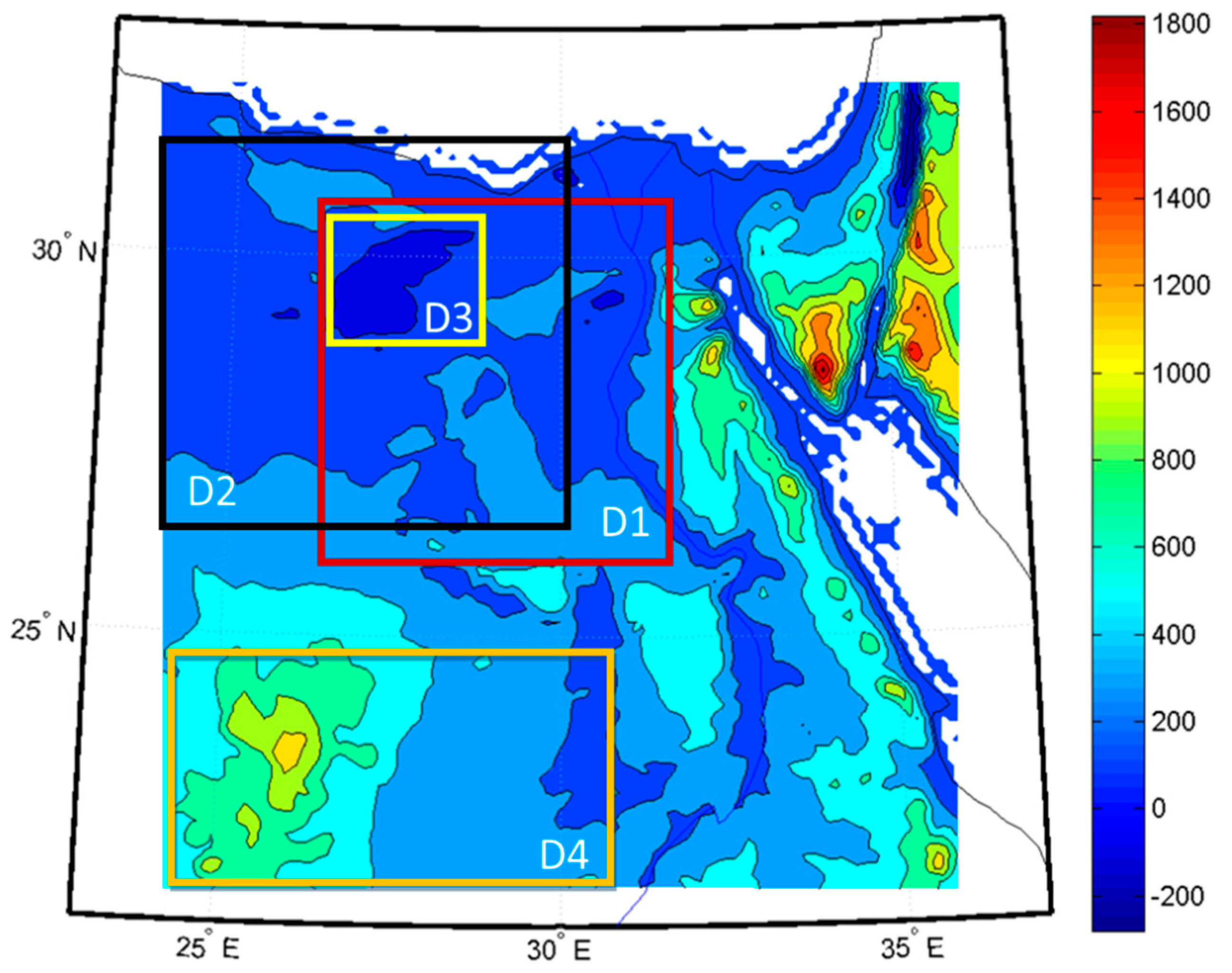
As mentioned before, the four subdomains D1, D2, D3, and D4 (Figure 1) are used to support the interpretation and validation of the model’s results. For the dust events of January 2004 and March 2013, the average of dust load is calculated over D1 and D2, respectively, while the average of AOD was validated over the same domains using MODIS results. Over Qattara Depression (D3), the soil texture types shown in the map of Figure 2 are in agreement with the surface conditions mentioned in [39]. Using the Total Ozone Mapping Spectrometer (TOMS) data to identify the source of atmospheric soil dust, the southwestern end of the Qattara Depression (22°–23° N, 15°–17° E) was defined as an active region of dust source [40]. Later in this section, it will be shown that there is correlation between the high erosion areas, the dust emissions and the AOD (both are output from the model). The domain 4 was constructed to validate the optical properties output from the model. The boundaries of all sub-domains are included in

Table 6. Selected domains with their boundries in core of dust blume (D1 & D2), Qattara Depression (D3), and south west of Egypt (D4).

	Upper (N)	Lower (S)	Left (W)	Right (E)
D1	30.3°	26.3°	27°	31°
D2	31°	27.1°	24.8°	29.4°
D3	30.1°	28.35°	26.1°	29.02°
D4	24.5°	22°	34°	31°

.

5.1. Analysis of the Dust Storm Event of January 2004

The analysis approach involves investigating the intensity of dust load and PM types from using a different tuning coefficient. The impact of these coefficients on optical properties is also established in terms of simulating the AOD. Different error analysis is used.

5.1.1. Dust Load and Particulate Matter

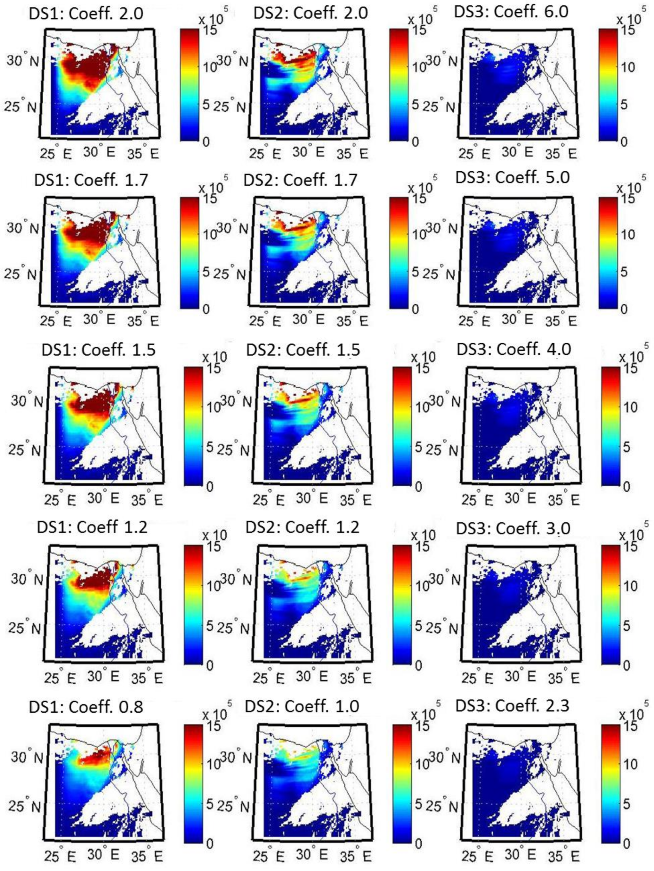
Spatial distribution of dust load from the model using the three dust schemes with different coefficients is shown in Figure 3. The maps are generated after applying a filter to exclude the areas that are not covered by MODIS AOD data. It can be seen that, by increasing the tuning coefficient for every dust scheme, more dust emission is produced at the core of the dust plume (in this case D1 as shown Figure 1). The average dust load within the D1 domain is included in

Table 7. Average dust load in (μg/m²) over domain D1 for dust storm January 2004.

Scheme	Coeff	Average Dust Load (μg/m2)
DS1	2.0	1.77 × 106
	1.7	1.53 × 106
	1.5	1.36 × 106
	1.2	1.11 × 106
	0.8	7.54 × 105
DS2	2.0	7.84 × 105
	1.7	6.79 × 105
	1.5	6.07 × 105
	1.2	4.95 × 105
	1.0	4.19 × 105
DS3	6.0	1.01 × 105
	5.0	8.83 × 104
	4.0	7.44 × 104
	3.0	6.08 × 104
	2.3	4.62 × 104

. It is seen that DS1 produces the highest dust load and the Coeff. 2 generates the highest values within DS1 (1.77 × 10⁶ μg/m²). On the other hand, DS3 generates low dust load with Coeff. 2.3 generating the lowest value (4.62 × 10⁴ μg/m³).

The spatial distribution of PM₁₀ and PM_2.5 for the setup that generates the highest dust load scheme (DS1 with Coeff. 2.0) is investigated in Figure 4. Both PM₁₀ and PM_2.5 maps confirm their high values within the domain D1, and particularly D3, with significantly higher value of PM₁₀. The average PM₁₀ and PM_2.5 within the D1 domain are 1.10 × 10⁴ and 2.22 × 10³ μg/m³, respectively. Recall that D3 is associated with high erosion scale factor (Figure 2), which means that the core of the dust storm of January 2003 features locally emitted dust.

5.1.2. Aerosol Optical Properties

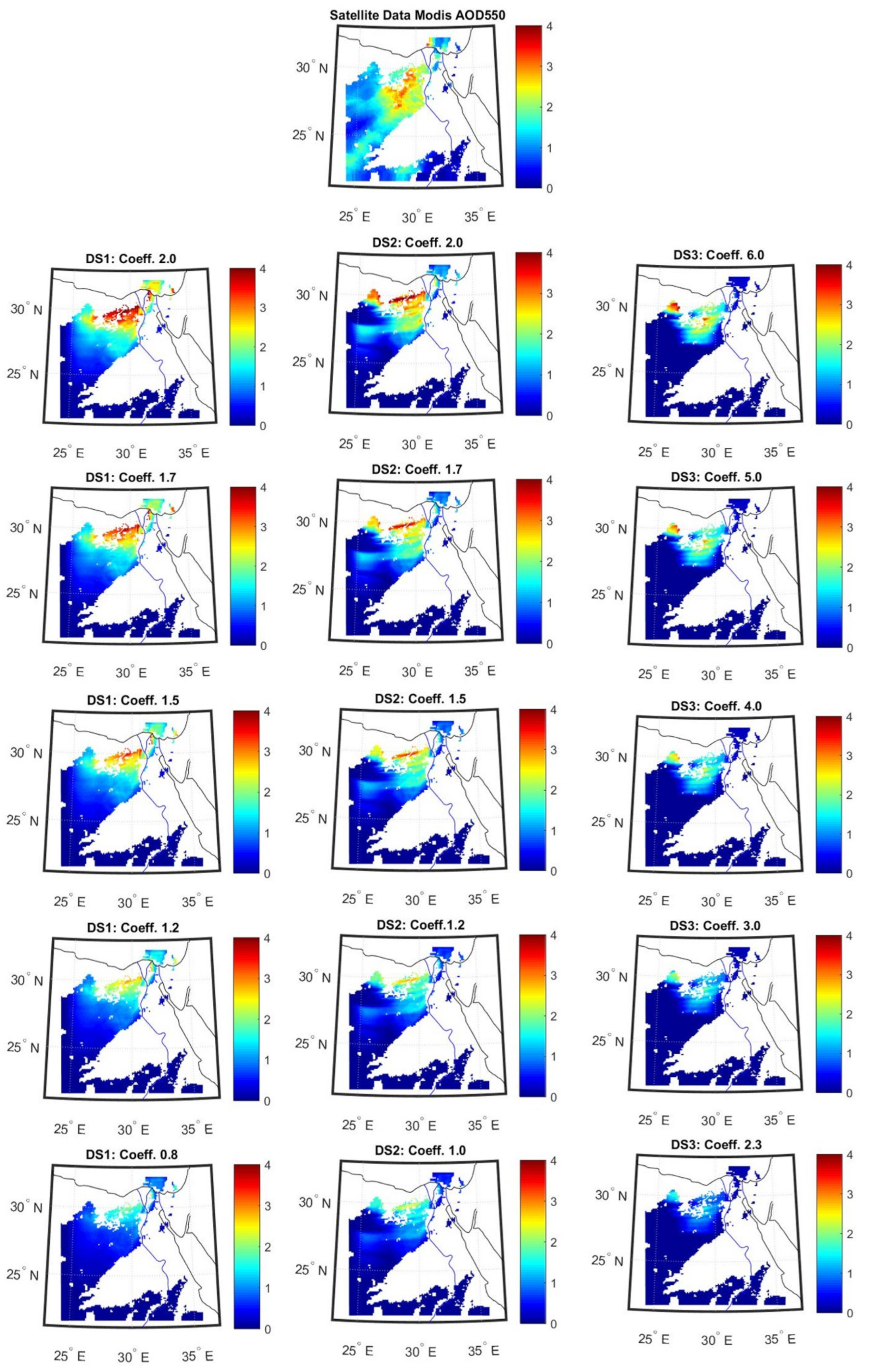
The investigation of the optical properties includes AOD and SSA from both MODIS and the fifteen-model simulation at hour 11:00 am (local time), as shown at Figure 5. MODIS identifies the core of the dust storm in the western desert and its peripherals in the surrounding areas. For all schemes, increasing the tuning coefficient leads to increase in AOD distribution within the core of the storm (D1 in Figure 1). The DS1 with Coeff 2.0 produces the closest average AOD (2.13 versus 2.29 from the scheme and MODIS, respectively). It is interesting to note the bigger difference between the MODIS and the same scheme when averaged over the entire country (0.81 versus 1.59, respectively). Note that the severe event of January 2004 covers mainly part of the western desert only.

Figure 6 shows AOD from MODIS versus all fifteen model simulations, averaged over Egypt and the domain D1. The Model’s performance over D1 is better than the entire country. Both DS1 and DS2 produce closer results to MODIS estimates than DS3. Results are always better when higher coefficients are used. Although DS3 highly underestimates AOD over Egypt, it produces reasonable agreement with MODIS over the effective area of the severe event. Further increase of the tuning coefficient (beyond 6.0) is expected produce better agreement.

MODIS was able to capture a relatively high AOD in the south west corner of Egypt within the domain D4 where none of the three emission model schemes was able to reproduce. However, the schemes did not produce high dust emission in this area (can be verified in Figure 2). This domain features a mountain that is covered by carboniferous rock. The failure of the schemes is because the dust source affecting this area is not included in the current setup domain; i.e., a boundary condition issue. The source is the Bodele Depression, which is located at southern edge of the Sahara Desert in north central Africa south of Chad (16° N–18° N) and (15° E–19° E). Impact of the modifying the boundary conditions by including other dust source will be shown in a future study.

The Comparison of SSA between MODIS and the model gives almost the same spatial distribution over the entire of Egypt, with SSA from MODIS was 0.952 and from the model using either DS1 or DS2 was 0.92. Nevertheless, SSA from using DS3 was around 0.8.

5.1.3. Results Validation

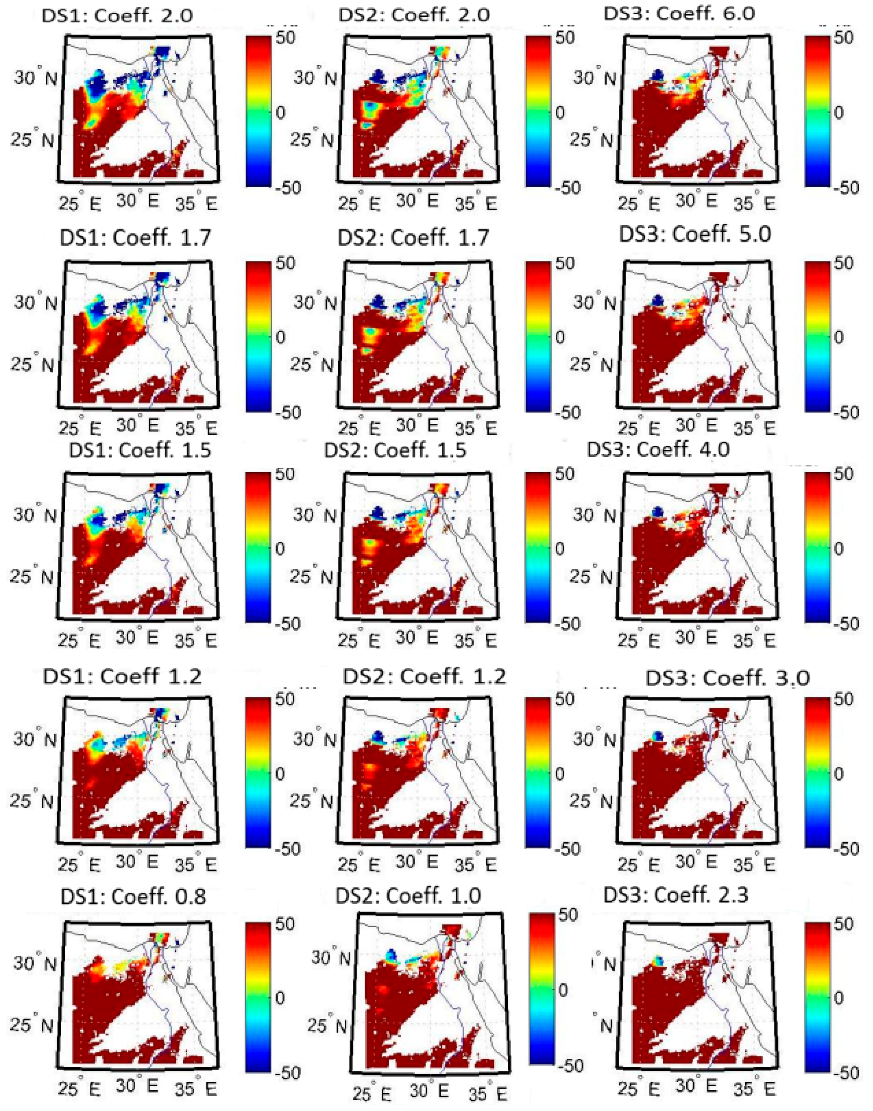
The event of January 2004 was validated only against MODIS data since AERONET data were not available. Two approaches to quantify the error are presented. In the first, the spatial distribution of the percentage error (MODIS minus Model AOD) is calculated while using Equation (4). Results are shown in Figure 7. In general, DS3 underestimates AOD almost everywhere, regardless of the tuning coefficient and less sensitive to sand/clay cover and the erosion factor, as shown in the maps in Figure 2. DS1 also underestimates MODIS AOD though it starts to match the satellite estimates when the tuning coefficient is set to 1.5. By increasing the tuning coefficient beyond 1.7, DS1 starts to overestimate the AOD. Careful examination of the percentage error within the D1 domain using DS1 with tuning coefficient 1.5 reveals a diverse of overestimation and underestimation of the model. It is not a coincident that the soil texture map (Figure 2) also shows diversity in the same domain. The overestimation of the model (by almost 50%) corresponds to the clay loam cover. The underestimation corresponds to areas that are covered by loam.

The second validation approach involves comparing eigenvalue structures of the spatial distribution of modeled AOD image and the AOD image from MODIS. This has been applied for each emission scheme and the selected tuning coefficients. The degree of resemblance between the two images is assessed by comparing the highest subset of eigenvalues. The scheme that gives the closest values to the MODIS values (presumed to be the validation data) is the best. The same is repeated for SSA.

Quantitative assessment of the “closeness” of the model’s eigenvalues to MODIS is estimated using the roots mean square error (RMSE).

$$\mathrm{RMSE}=\sqrt{\left(\frac{1}{n}\right){{\displaystyle \sum }}_{j=1}^{n}eigenvaluesX{}_{eachscheme}–eigenValuesX{}_{MODIS}}$$

(7)

where X will be either AOD or SSA.

The eigenvalues for AOD and SSA are plotted in Figure 8. According to the inset in Figure 8a, the first dominant eigenvalue of DS1 with Coeff. 1.7 matches those of MODIS, while the eigenvalue that was computed using tuning Coeff.2.0 produced a higher eigenvalue corresponding to the higher AOD from MODIS image as seen in Figure 5. Except for the first few image eigenvalues, all other eigenvalues, which play a secondary role in the comparison, underestimates those from MODIS.

On the other hand, eigenvalues of SSA for each member of three dust schemes are shown to cluster, as in Figure 8b. In general, the difference between the values from the model and MODIS are larger for SSA than AOD. Unlike the AOD case, the DS3 has the closest values to MODIS in terms of SSA estimation. The eigenvalue structures showed low sensitivity to the variation of coefficients for each dust scheme

Table 8. Roots mean square error (RMSE) for AOD and SSA of eigenvalues between all the model simulations and MODIS for dust storm January 2004.

Scheme	RMSE AOD Eigenvalues	RMSE SSA Eigen Values
DS1 Coeff 2.0	0.206097	0.575826
DS1 Coeff 1.7	0.213703	0.575952
DS1 Coeff 1.5	0.238308	0.57599
DS1 Coeff 1.2	0.290285	0.576174
DS1 Coeff 0.8	0.386937	0.576487
DS2 Coeff 2.0	0.254319	0.583857
DS2 Coeff 1.7	0.291054	0.584063
DS2 Coeff 1.5	0.32093	0.584154
DS2 Coeff 1.2	0.368645	0.584405
DS2 Coeff 1.0	0.40493	0.584651
DS3 Coeff 6.0	0.480568	0.541646
DS3 Coeff 5.0	0.495943	0.542941
DS3 Coeff 4.0	0.512923	0.544668
DS3 Coeff 3.0	0.531039	0.546865
DS3 Coeff 2.3	0.550296	0.550011

includes the RMSE values for AOD and SSA from using each dust scheme for all of the selected tuning coefficients. For the case of AOD, DS1 with coeff. 2.0 has lowest RMSE (0.206), while DS3 with coeff. 2.3 has highest RMSE (0.550). On the other hand, for SSA, the scheme DS3 with coeff. 6.0 produced lowest RMSE (0.542) and scheme DS2 with coeff. 1.0 has highest RMSE (0.585). Judging the best dust scheme cannot be based on RMSE of the eigenvalue of optical properties only. The difference between the spatial average of the properties from the model and satellite estimates over selected domains also contribute to the evaluation. This identifies the performance of the model in relation to the surface cover and the emission of different dust types.

5.2. Analysis of Dust Storm Event of March 2013

Unlike the previous case study of January 2004 where the dust storm was triggered by southwesterly wind (i.e., the origin was from the core of the western desert), this case study (31 March 2013) has its dust that originated from the north part of the desert, carried by northwesterly wind. The same analysis approach is used in this case study.

5.2.1. Dust Load and Particulate Matter

Spatial distributions of dust load for six selected model’s configurations with different tuning coefficient are shown in Figure 9. In terms of the spatial distributions of dust load, all of the schemes have the capability to capture higher dust load within the domain D2 (core of the dust plume shown in Figure 1), yet with different intensity. Similar to case study 1, DS3 has the lowest capability to produce the dust load, while DS1 produces the highest dust load, but with a tuning coefficient 10 (very different than the coefficient 1.5 revealed in case study 1). Average dust load from all different schemes for each coefficient are shown in

Table 9. Average dust load in (μg/m²) over domain D2 for dust storm March 2013.

Scheme	Coeff.	Average Dust Load (μg/m2)
DS1	10	1.50 × 106
	8.0	1.21 × 106
	6.0	9.07 × 105
	4.0	6.07 × 105
	3.0	4.56 × 105
DS2	10.0	4.62 × 105
	8.0	3.75 × 105
	6.0	2.87 × 105
	4.0	1.95 × 105
	3.0	1.90 × 105
DS3	11.0	1.31 × 105
	10.0	1.20 × 105
	8.0	9.89 × 104
	6.0	7.69 × 104
	5.0	6.56 × 104

. Increasing the Tuning coefficient leads to increase of average dust loads. The highest dust load from using DS1 with coefficient 10 generates a value 1.50 × 10⁶ μg/m², while the lowest average dust load was emitted by scheme DS3 with coefficient 5.0 (6.56 × 10⁴ μg/m²).

The composition of dust load for scheme DS1 with Coeff. 10 in terms of PM₁₀ and PM_2.5 is shown in Figure 10. DS1 Is selected because it has lowest root mean square error, as shown later in Section 5.2.3. Similar to the previous case study, PM₁₀ has higher intensity than PM_2.5. The average of PM₁₀ inside domain D2 is 2.07 × 10⁴ μg·m³, while PM_2.5 has average value than 4.190 × 10³ μg·m³. This event has higher dust load than the previous case study. Moreover, since the PM₁₀ load is higher in this case than the previous case, the tuning coefficient that is needed to reproduce the AOD (presented later) is higher than the previous case of January 2013.

5.2.2. Aerosol Optical Properties

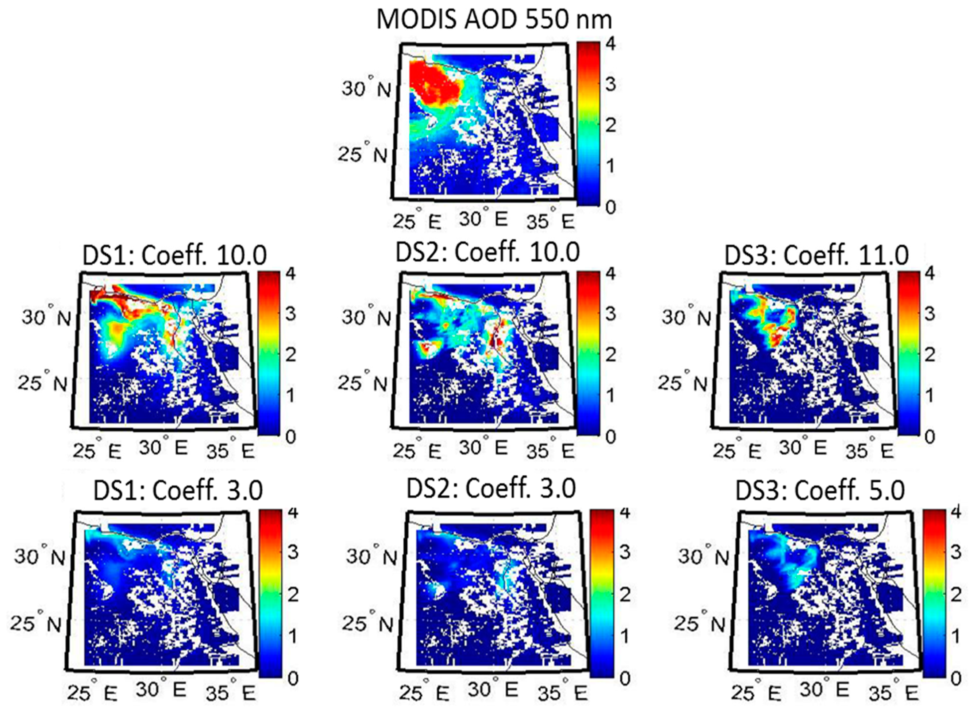
The spatial distribution of aerosol optical depth (AOD) from the three selected schemes with selected coefficients was compared to AOD from MODIS at hour 11:00 am local time. Results are shown at Figure 11. AOD from MODIS shows high values at the North West corner of Egypt. This is the core of the dust plume of the Mach 2013 event. The source of this storm is located in the Eastern Libyan Desert, which is defined in the global source of dust [40]. This area extends from the eastern Libyan into western Egypt. The dust source in this area is active for most of the year [40]. MODIS data shows that AOD reaches 3.5 over a large bulk area through domain D2. From the top left panel of the model’s results in Figure 11, it can be seen that the model can reproduce values close to those that were obtained from MODIS only in the north part of domain D2, which is covered by clay loam. It produces much lower values in the southern part of D2, which is mainly covered by loamy sand (see Figure 2 and Table 5).

Table 10. Average AOD over domain D2 from using all the schemes with all coefficients, in addition to MODIS AOD at 550 nm wavelength the dust storm of Mrach 2013.

Scheme	Average AOD
DS1 Coeff. 10	1.7135
DS1 Coeff. 8.0	1.3768
DS1 Coeff. 6.0	1.0372
DS1 Coeff. 4.0	0.6965
DS1 Coeff. 3.0	0.525
DS2 Coeff. 10.0	1.2764
DS2 Coeff. 8.0	1.0391
DS2 Coeff. 6.0	0.796
DS2 Coeff. 4.0	0.5435
DS2 Coeff. 3.0	0.4136
DS3 Coeff. 11.0	1.5121
DS3 Coeff. 10.0	1.0564
DS3 Coeff. 8.0	0.8604
DS3 Coeff. 6.0	0.6581
DS3 Coeff. 5.0	0.5545
MODIS	2.4105

includes the average AOD over D2 from using all of the tested dust schemes and coefficients. Increasing the tuning coefficients in any dust scheme leads to a noticeable increase in AOD. The average AOD from MODIS over the bulk of the domain D2 is 2.41, while the average from DS1 with coefficient 10 is 1.71 and from DS3 with coefficient 11.0 is 1.51. It should be noted, however, that the spatial distribution of AOD from DS3 is far from that of MODIS. This implies that, if a higher coefficient is used (>11.0), it may simulate the AOD within the dust storm area better. Nevertheless, it is almost sure that further increase of the coefficient will not provide accurate simulation of AOD outside the area of the dust storm. It seems that adjusting the coefficient in any dust scheme may not lead to acceptable spatial distribution of AOD under various soil texture. Recall that the approach of this study has been designed to address the evaluation of WRF-Chem. in response to dust emission only, not other chemical of other aerosol emissions. Modifying the boundary conditions by including other dust sources outside Egypt in this case study may have impact the spatial distibution of AOD.

5.2.3. Results Validation

Maps of the spatial distribution of the percentage error of AOD (MODIS minus Model) for the same selected six configurations is shown in Figure 12. Similar to the first case study (Figure 7), the model underestimates AOD in most areas. Increasing the tuning coefficient reduce the error. It is apparent that DS1 with tuning coefficient 10 produces closer AOD to MODIS though a sharp contrast between the model’s underestimation and overestimation is visible within D2 (the dust event area in Figure 2).

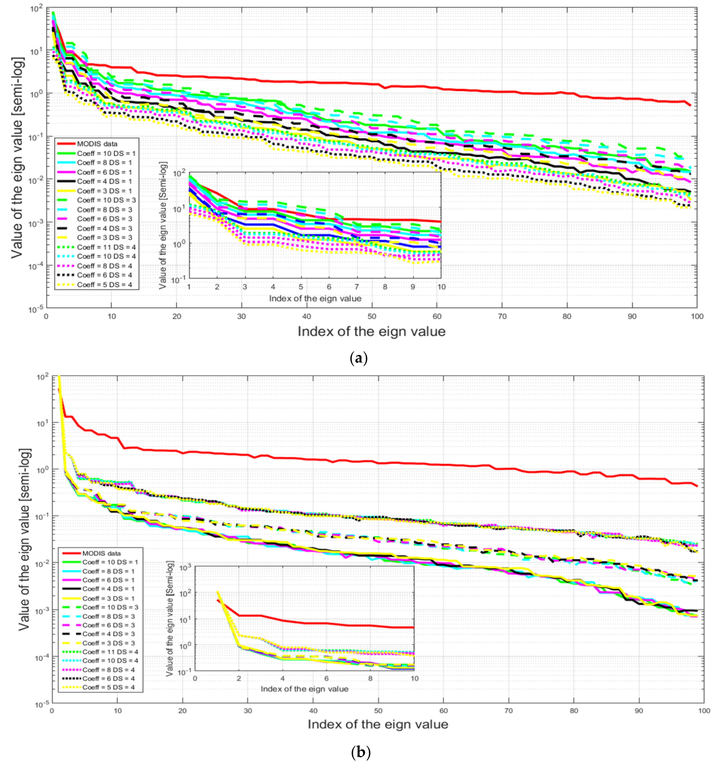
Results from the eigenvalue structure method of validation (Section 5.1.3) are shown in Figure 13 for AOD. For the first eigenvalue from using DS1 and DS2 with the higher coefficient produce higher values than MODIS. This confirms the superiority of these two schemes. Except for the first few eigenvalues, all the other eigenvalues, which play a secondary role in the comparison, underestimates those from MODIS. The RMSE of difference of eigenvalues between the model and MODIS results, for AOD and SSA parameters, are given in

Table 11. RMSE for AOD and SSA of eigen values between all model simulations and MODIS for dust storm March 2013.

Scheme	RMSE AOD Eigen Values	RMSE SSA Eigen Values
DS 1 Coeff 10	0.243746	0.632762
DS 1 Coeff 8.0	0.19663	0.633088
DS 1 Coeff 6.0	0.254537	0.633551
DS 1 Coeff 4.0	0.372464	0.634322
DS 1 Coeff 3.0	0.439912	0.634935
DS 2 Coeff 10	0.276502	0.640653
DS 2 Coeff 8.0	0.193523	0.641138
DS 2 Coeff 6.0	0.212372	0.641789
DS 2 Coeff 4.0	0.327641	0.642795
DS 2 Coeff 3.0	0.402051	0.643578
DS 3 Coeff 11	0.519369	0.591345
DS 3 Coeff 10	0.53047	0.592293
DS 3 Coeff 8.0	0.552759	0.594754
DS 3 Coeff 6.0	0.575328	0.598174
DS 3 Coeff 5.0	0.586879	0.600431

. For AOD, the minimum value is found when using DS1 with coefficient 8 (0.197), while DS3 with coefficient 5 has the highest RMSE with (0.587).

Similar to the first case study, the eigenvalues for the SSA are also shown to be cluster. The eigenvalue structures show low sensitivity to the variation of coefficients for each dust scheme. For the first eigenvalue, all of the schemes overestimate the value with respect to MODIS. After that, all the eigenevalues are lower than those from MODIS. The difference between the values from the model and MODIS are larger for SSA than AOD. Unexpectedly, DS3 has the closest values to MODIS in terms of SSA estimation. Table 11 shows that all RMSE are above 0.55 with max RMSE around 0.633 for scheme DS1.

AERONET data from the station in Cairo was available for the dust event of March 2013. AOD from MODIS, AERONET, and the model with the tested dust schemes with the selected tuning coefficients are presented on Figure 14. MODIS and the model’s results are averaged over 50 × 50 km around Cairo. It is shown that MODIS underestimates the AOD over Cairo during this event (considering that AERONET provides the closest to the truth). Both DS1 and DS2 with coefficient 4 have the best capability to capture the AOD over Cairo.

6. Conclusions and Future Work

The WRF-chem model has been used to simulate two severe dust storms over Egypt occurred on 22 January 2004 and 31 March 2013. The first dust storm blew from south west of Egypt and was amplified due to an internal dust source that was located at Qattara Depression, which contains high clay and Sand Fractions. The storm reached its highest intensity over the Qattara Depression. This Depression works as a catalyst for the dust storms. The second dust storm came from North West of Egypt and passes over Qattara Depression. The model grid used in the study was 10 km in order to match the spatial grid spacing of MODIS level 2 aerosol products. Admittedly, this does not provide details of the spatial distribution of the dust aerosol. Nevertheless, it satisfies the purpose of the study in identifying the best dust scheme with the best coefficients that simulate the dust event in terms of matching the two products of AOD and SSA from the model against MODIS estimates. Once this is established, models run at finer grid resolution to capture details will be possible.

The present study confirms the conclusions from previous studies that WRF-chem underestimates AOD during severe dust storm when using any of the three dust schemes: GOCART, GOCART-AFWA, and GOCART-UOC. In an attempt to improve the models’ performance, the study applied the model using each dust scheme with a selected set of tuning coefficients in vertical dust flux Equations. Increasing the tuning coefficient will increase the dust emission and that leads to improve the AOD prediction. Tuning these coefficients has no physical basis and is valid for deterministic model setup. The selection for the coefficients was not based on any physical criterion. Different tuning coefficients set were required for each case study, depending on the origin and the composition of the dust storm.

Performance of WRF-Chem model was validated against MODIS data in terms of two optical aerosol parameters: AOD and SSA. AERONET data was available for validation only for the second dust storm event in March 2013. It was shown that the schemes DS1 and DS2 with coefficient value 4.0 have the nearest values to the AOD from the AERONET station in Cairo. However, the spatial distribution of AOD from MODIS was considered to be the target criterion for assessing the tuning. This is the best that can be done in absence of ground observation.

In order to compare between different dust schemes with different tuning coefficient, the comparison between the structure of the eigenvalues of the model and the MODIS distribution images are used. This was applied to the AOD and SSA parameters. RMSE for these eigenvalues were investigated. GOCART dust scheme gives the better performance for simulating the AOD over Egypt for both dust event cases in terms of the spatial distribution and the average of AOD.

In the January 2004 case study, the average AOD from MODIS at the core of the dust storm was 2.29, while GOCART with coefficient 2.0 was the closest scheme with 2.13. On the other hand, for the case study of March 2013, the average AOD from MODIS was 2.4 at the core of the dust plume while GOCART with coefficient 10 produced the closest average of AOD, which was 1.71.

As a result, the GOCART scheme with coefficient 2.0 gave the lowest RMSE (0. 206) for the case of January and with coefficient 8.0 the lowest RMSE (0.192) for the second dust case at 2013. The dust schemes GOCART-AFWA and GOCART-UOC always provide underestimation for all the current tuning set and they need more increase for the tuning coefficients.

Dust emission depends on the soil texture. Therefore, for the same domain, different values for the tuning coefficients should be implemented based on the soil texture. Otherwise, the application may lead to overestimating AOD over the areas with high clay fraction, such as in parts of the Qattara Depression. It may also underestimate AOD in other areas that may contain much sand.

It is shown that the spatial geographic domain setup should have impact on the current simulation. The current setup simulation in this study includes only one source of dust emissions (from Qattara Depression). Other sources were not included, such as the one in Libya’s eastern desert and the Bodele Depression at Chad. Both sources have impact on the dust storm pattern over Egypt. So, the spatial domain should be extended to include both sources. Different tuning methods could be implemented to tune the dust schemes include modifying values of the threshold of surface wind, friction velocity, or surface roughness. Data assimilation methods should modify the surface wind, which has direct impact if the tuning coefficient method was used to tune the model. Detailed and empirical soil map for Egypt also will impact the results as well.

References

1. Goudie, A.S.; Middleton, N.J. Desert Dust in the Global System; Springer: Berlin/Heidelburg, Germany, 2006; 287p. [Google Scholar]
2. Thomas, D.S.G. Aeolian Landscapes and Bedforms. In Arid Zone Geomorphology: Process, Form and Change in Drylands, 3rd ed.; Thomas, D.S.G., Ed.; Wiley: Hoboken, NJ, USA, 2011; pp. 427–454. [Google Scholar]
3. Tegen, I.; Hollrig, P.; Chin, M.; Fung, I.; Jacob, D.; Penner, J. Contribution of different aerosol species to the global aerosol extinction optical thickness: Estimates from model results. J. Geophys. Res. 1997, 102, 23895–23915. [Google Scholar] [CrossRef] [Green Version]
4. Levin, Z.; Ganor, E.; Gladstein, V. The effects of desert particles coated with sulfate on rain formation in the eastern Mediterranean. J. Appl. Meteorol. 1996, 35, 1511–1523. [Google Scholar] [CrossRef]
5. Dentener, F.J.; Carmichael, G.R.; Zhang, Y.; Lelieveld, J.; Crutzen, P.J. Role of mineral aerosol as a reactive surface in the global troposphere. J. Geophys. Res. 1996, 101, 22869–22889. [Google Scholar] [CrossRef]
6. United Nations Environment Programme (UNEP); World Meteorological Organization (WMO); United Nations Convention to Combat Desertification (UNCCD). Global Assessment of Sand and Dust Storms; United Nations Environment Programme: Nairobi, Kenya, 2016. [Google Scholar]
7. Grell, G.A.; Peckham, S.E.; Schmitz, R.; McKeen, S.A.; Frost, G.; Skamarock, W.C.; Eder, B. Fully coupled ‘‘online’’ chemistry within the WRF model. Atmos. Environ. 2005, 39, 6957–6975. [Google Scholar] [CrossRef]
8. Kumar, R.; Barth, M.C.; Pfister, G.G.; Naja, M.; Brasseur, G.P. WRF-Chem simulations of a typical pre-monsoon dust storm in northern India: influences on aerosol optical properties and radiation budget. Atmos. Chem. Phys. 2014, 14, 2431–2446. [Google Scholar] [CrossRef] [Green Version]
9. Rizza, U.; Barnaba, F.; Miglietta, M.M.; Mangia, C.; Di Liberto, L.; Dionisi, D.; Costabile, F.; Grasso, F.; Gobbi, G.P. WRF-Chem model simulations of a dust outbreak over the central Mediterranean and comparison with multi-sensor desert dust observations. Atmos. Chem. Phys. 2017, 17, 93–115. [Google Scholar] [CrossRef] [Green Version]
10. Flaounas, E.; Kotroni, V.; Lagouvardos, K.; Klose, M.; Flamant, C.; Giannaros, T.M. Sensitivity of the WRF-Chem (V3.6.1) model to different dust emission parametrisation: Assessment in the broader Mediterranean region. Geosci. Model Dev. 2017, 10, 2925–2945. [Google Scholar] [CrossRef]
11. El-Metwally, M.; Alfaro, S.C.; Wahab, M.M.A.; Zakey, A.S.; Chatenet, B. Seasonal and inter-annual variability of the aerosol content in Cairo (Egypt) as deduced from the comparison of MODIS aerosol retrievals with direct AERONET measurements. Atmos. Res. 2010, 97, 14–25. [Google Scholar] [CrossRef]
12. El-Askary, H.; Kafatos, M. Dust Storm and Black Cloud Influence on Aerosol Optical Properties over Cairo and the Greater Delta Region, Egypt. Int. J. Remote Sens. 2008, 29, 7199–7211. [Google Scholar] [CrossRef]
13. Marey, H.S.; Gille, J.C.; El-Askary, H.M.; Shalaby, E.A.; El-Raey, M.E. Study of the formation of the “black cloud” and its dynamics over Cairo, Egypt, using MODIS and MISR sensors. J. Geophys. Res. 2010, 115, 1–10. [Google Scholar] [CrossRef]
14. El-Metwally, M.; Alfaro, S.C.; Abdel Wahab, M.M.; Favez, O.; Mohamed, Z.; Chatenet, B. Aerosol properties and associated radiative effects over Cairo (Egypt). Atmos. Res. 2011, 99, 263–276. [Google Scholar] [CrossRef]
15. Mahmoud, K.F.; Alfaro, S.C.; Favez, O.; Abdel Wahab, M.M.; Sciare, J. Origin of black carbon concentration peaks in Cairo (Egypt). Atmos. Res. 2008, 89, 161–169. [Google Scholar] [CrossRef]
16. Shokr, M.; Eltahan, M.; Ibrahim, A.; Steiner, A.; Gad, N. Long-term, high resolution survey of atmospheric aerosols over Egypt with NASA’s MODIS data. Remote Sens. 2017, 9, 1027. [Google Scholar] [CrossRef]
17. Ginoux, P.; Chin, M.; Tegen, I.; Prospero, J.M.; Holben, B.; Dubovik, O.; Lin, S.-J. Sources and distributions of dust aerosols simulated with the GOCART model. J. Geophys. Res. 2001, 106, 20255–20273. [Google Scholar] [CrossRef] [Green Version]
18. Darmenova, K.; Sokolik, I.N.; Shao, Y.; Marticorena, B.; Bergametti, G. Development of a physically based dust emission modulewithin the Weather Research and Forecasting (WRF) model: Assessment of dust emission parameterizations and input parameters for source regions in Central and East Asia. J. Geophys. Res. 2009, 114, D14201. [Google Scholar] [CrossRef]
19. Kang, J.-Y.; Yoon, S.-C.; Shao, Y.; Kim, S.-W. Comparison of vertical dust flux by implementing three dust emission schemes in WRF/Chem. J. Geophys. Res. 2011, 116. [Google Scholar] [CrossRef] [Green Version]
20. Skamarock, W.C.; Klemp, J.B.; Dudhia, J.; Gill, D.O.; Barker, D.M.; Wang, W.; Powers, J.G. A Description of the Advanced Research WRF Version 3; NCAR Technical Notes-475+STR; National Center for Atmospheric Research: Boulder, CO, USA, 2008. [Google Scholar]
21. Skamarock, W.C.; Klemp, J.B.; Dudhia, J.; Gill, D.O.; Barker, D.M.; Wang, W.; Powers, J.G. A Description of the Advanced Research WRF Version 2; NCAR Technical Notes-468+STR; National Center for Atmospheric Research: Boulder, CO, USA, 2005. [Google Scholar]
22. Freitas, S.R.; Longo, K.M.; Alonso, M.F.; Pirre, M.; Marecal, V.; Grell, G.; Stockler, R.; Mello, R.F.; Gácita, M.S. PREP-CHEM-SRC—1.0: A preprocessor of trace gas and aerosol emission fields for regional and global atmospheric chemistry models. Geosci. Model Dev. 2011, 4, 419–433. [Google Scholar] [CrossRef] [Green Version]
23. Thompson, G.; Eidhammer, T. A study of aerosol impacts on clouds and precipitation development in a large winter cyclone. J. Atmos. Sci. 2014, 71, 3636–3658. [Google Scholar] [CrossRef]
24. Mlawer, E.J.; Taubman, S.J.; Brown, P.D.; Iacono, M.J.; Clough, S.A. Radiative transfer for inhomogeneous atmospheres: RRTM, a validated correlated–k model for the longwave. J. Geophys. Res. 1997, 102, 16663–16682. [Google Scholar] [CrossRef]
25. Tewari, M.; Chen, F.; Wang, W.; Dudhia, J.; LeMone, M.A.; Mitchell, K.; Ek, M.; Gayno, G.; Wegiel, J.; Cuenca, R. Implementation and Verification of the Unified NOAH Land Surface Model in the WRF Model. In Proceedings of the 20th Conference on Weather Analysis and Forecasting/16th Conference on Numerical Weather Prediction, Seattle, WA, USA, 11–15 January 2004; pp. 11–15. [Google Scholar]
26. Hong, S.-Y.; Dudhia, J.; Chen, S.-H. A revised approach to ice-microphysical processes for the bulk parameterization of cloud and precipitation. Mon. Weather Rev. 2004, 132, 103–120. [Google Scholar] [CrossRef]
27. Paulson, C.A. The mathematical representation of wind speed and temperature profiles in the unstable atmospheric surface layer. J. Appl. Meteorol. 1970, 9, 857–861. [Google Scholar] [CrossRef]
28. Grell, G.A.; Devenyi, D. A generalized approach to parameterizing convection combining ensemble and data assimilation techniques. Geophys. Res. Lett. 2002, 29, 1693. [Google Scholar] [CrossRef]
29. White, B.R. Soil transport by winds on Mars. J. Geophys. Res. 1979, 84, 4643–4651. [Google Scholar] [CrossRef]
30. Marticorena, B.; Bergametti, G. Modeling the atmospheric dust cycle: 1. Design of a soil-derived dust emission scheme. J. Geophys. Res. 1995, 100, 16415–16430. [Google Scholar] [CrossRef]
31. Marticorena, B.; Bergametti, G.; Gillette, D.; Belnap, J. Factors controlling threshold friction velocity in semiarid and arid areas of the United States. J. Geophys. Res. Atmos. 1997, 102, 23277–23288. [Google Scholar] [CrossRef]
32. Laurent, B.; Marticorena, B.; Bergametti, G.; Mei, F. Modeling mineral dust emissions from Chinese and Mongolian deserts. Glob. Planet. Chang. 2006, 52, 121–141. [Google Scholar] [CrossRef]
33. Flaounas, E.; Kotroni, V.; Lagouvardos, K.; Klose, M.; Flamant, C.; Giannaros, T.M. Assessing atmospheric dust modelling performance of WRF-Chem over the semi-arid and arid regions around the Mediterranean. Atmos. Chem. Phys. Discuss. 2016. [Google Scholar] [CrossRef]
34. Remer, L.A.; Kaufman, Y.J.; Tanré, D.; Mattoo, S.; Chu, D.A.; Martins, J.V.; Li, R.-R.; Ichoku, C.; Levy, R.C.; Kleidman, R.G.; et al. The MODIS aerosol algorithm, products and validation. J. Atmos. Sci. 2005, 62, 947–973. [Google Scholar] [CrossRef]
35. Remer, L.A.; Kleidman, R.; Levy, R.; Kaufman, Y.; Tanre, D.; Mattoo, S.; Martins, J.V.; Ichoku, C.; Koren, I.; Yu, H.; et al. Global aerosol climatology from the MODIS satellite sensors. J. Geophys. Res. Atmos. 2008, 113, D14S07. [Google Scholar] [CrossRef]
36. Davis, R.O.E.; Bennett, H.H. Grouping of Soils on the Basis of Mechanical Analysis; United States Department of Agriculture: Washington, DC, USA, 1927.
37. Soil Survey Division Staff. Soil Survey Manual USDA Handbook No.18; US Government Printing Office: Washington, DC, USA, 1993.
38. Verruijt, A. Soil Mechanics Book; Delft University of Technology: Delft, The Netherlands, 2001. [Google Scholar]
39. Guth, P.L. Military Geology in War and Peace: An Introduction. In Military Geology in War and Peace; Underwood, J.R., Jr., Guth, P.L., Eds.; Geological Society of America: Boulder, CO, USA, 1998; Volume 13. [Google Scholar]
40. Prospero, J.M.; Ginoux, P.; Torres, O.; Nicholson, S.E.; Gill, T.E. Environmental characterization of global sources of atmospheric soil dust identified with the NIMBUS 7 total ozone mapping spectrometer (TOMS) absorbing aerosol product. Rev. Geophys. 2002, 40. [Google Scholar] [CrossRef]
Figure 1. A map of Egypt that includes the configured geographic domain for the WRF model and Terrain height (in m as shown in the color bar). The four sub-domains D1, D2, D3, and D4 are used in the interpretation and validation of the model’s output as explained later in the text.
Atmosphere 09 00246 g001
Figure 2. Spatial distribution of the erosion factor (a) and soil texture classification (b) over Egypt, used as input to the model. The 16 categories of the soil are presented in Table 5. Location of AERONET stations (C1, C2, C3 and C4) are indicated on the Figure 2a.
Atmosphere 09 00246 g002
Figure 3. Spatial distribution of dust load over Egypt (μg/m2) for the dust storm event of January 2004. The three columns represent the three dust schemes (DS) and each row includes output from using the given coefficient. White areas are pixels not covered by Moderate-resolution Imaging Spectroradiometer Aerosol Optical Depth (MODIS AOD) data.
Atmosphere 09 00246 g003
Figure 4. Spatial distribution of the PM10 (a) and PM2.5 (b) during the dust storm of January 2004 from DS1 with coeff. 2.0. Domains D1 and D3 are shown. The color bar represents the particle density (μg/m3) multiplied by 104.
Atmosphere 09 00246 g004
Figure 5. Spatial distribution of AOD over Egypt from MODIS (top middle) and the fifteen simulations from the model at 11:00 am (local time) for the dust event of January 2004. The color bar applies to all panels. The missing pixels in MODIS data (white areas) are excluded in the model data.
Atmosphere 09 00246 g005
Figure 6. Average AOD from MODIS vs. all fifteen model simulation over (a) Egypt (b) Domain D1.
Atmosphere 09 00246 g006
Figure 7. The distribution of spatial error in (%) between MODIS (as reference) and the Model AOD using fifteen simulations for the January 2004 dust storm (panel arrangement is the same as shown in Figure 2).
Atmosphere 09 00246 g007
Figure 8. Eigen values for (a) AOD (top) and (b) single scattering albedo (SSA) (bottom) distributions from MODIS and Model’s results using all the dust schemes for the dust event of January 2004.
Atmosphere 09 00246 g008
Figure 9. The Spatial distribution of dust load over Egypt using six selected DS and tuning coefficients for dust storm at 31 March 2013.
Atmosphere 09 00246 g009
Figure 10. Spatial distribution of the PM10 (a) and PM2.5 (b) during the dust storm of 31 March 2013 from DS1 with coeff. 10.0. Domains D2 (the core of the dust storm) is marked. The color bar represents the particle density (μg/m3) multiplied by 104.
Atmosphere 09 00246 g010
Figure 11. The Spatial distribution of AOD from using the shown selected DS and tuning coefficients over Egypt on the day of the dust storm of 31 March 2013.
Atmosphere 09 00246 g011
Figure 12. The distribution of spatial error in (%) between MODIS (as reference) Model AOD using selected emission scheme and tuning coefficient for the event of March 2013.
Atmosphere 09 00246 g012
Figure 13. Eigenvalues for (a) AOD (top) and (b) SSA (bottom) distributions from MODIS and Model’s results using all dust schemes for the dust event of March 2013.
Atmosphere 09 00246 g013
Figure 14. Average AOD over Cairo from MODIS, AERONET and the WRF-Chem model with all different dust schemes and tuning coefficient. from during dust event of 31 March 2013.
Atmosphere 09 00246 g014