Cloud Area Distributions of Shallow Cumuli: A New Method for Ground-Based Images
by
 , and
, and
Jessica M. Kleiss
1,*, 
Erin A. Riley
1,
Charles N. Long
2,
Laura D. Riihimaki
3,
Larry K. Berg
3,
Victor R. Morris
3 and
Evgueni Kassianov
3,* 1
Environmental Studies, Lewis and Clark College, Portland, OR 97219, USA
2
Cooperative Institute for Research in Environmental Sciences, Boulder, CO 80309, USA
3
Pacific Northwest National Laboratory, Richland, WA 99354, USA
*
Authors to whom correspondence should be addressed.
Atmosphere 2018, 9(7), 258; https://doi.org/10.3390/atmos9070258
Submission received: 18 June 2018
/
Revised: 7 July 2018
/
Accepted: 9 July 2018
/
Published: 12 July 2018
(This article belongs to the Section Meteorology)
Abstract
:We develop a new approach that resolves cloud area distributions of single-layer shallow cumuli from ground-based observations. Our simple and computationally inexpensive approach uses images obtained from a Total Sky Imager (TSI) and complementary information on cloud base height provided by lidar measurements to estimate cloud equivalent diameter (CED) over a wide range of cloud sizes (about 0.01–3.5 km) with high temporal resolution (30 s). We illustrate the feasibility of our approach by comparing the estimated CEDs with those derived from collocated and coincident high-resolution (0.03 km) Landsat cloud masks with different spatial and temporal patterns of cloud cover collected over the Atmospheric Radiation Measurement (ARM) Southern Great Plains (SGP) site. We demonstrate that (1) good (~7%) agreement between TSI and Landsat characteristic cloud size can be obtained for clouds that fall within the region of the sky observable by the TSI and (2) large clouds that extend beyond this region are responsible for noticeable (~16%) underestimation of the TSI characteristic cloud size. Our approach provides a previously unavailable dataset for process studies in the convective boundary layer and evaluation of shallow cumuli in cloud-resolving models.
1. Introduction
Shallow cumuli are observed frequently over many continental and marine regions of the world. They consist mainly of small (<1 km) clouds [1,2] and thus represent a great challenge for both observational and model studies. Cloud horizontal size and its diurnal changes substantially influence complex surface-atmosphere interactions, including energy fluxes at the land-atmosphere boundary and the Earth’s radiation budget [3,4,5]. The cloud size distribution is used to calculate mass flux and energy transport in cloud models and also for model evaluation against observations.
Although the term “cloud horizontal size” is commonly used to refer to cloud chord length (CCL) derived from ground-based radar-lidar [6] or aircraft [7] data, model studies typically restrict the word “size” to describe cloud equivalent diameter (CED) of a given cloud area [8]. As a consequence, the data-derived CCL and model-predicted CED often cannot be compared directly especially at short temporal and spatial scales as recently shown by Romps and Vogelmann [9].
Satellite observations can be used to measure cloud area [10,11], though the accuracy of the cloud area measurements depends strongly on the spatial resolution of the satellite sensor and the most frequent cloud size [12]. In particular, the spatial resolution must be high enough to resolve the majority of clouds within a given scene. Since shallow cumuli are typically small (<0.4 km) [6,11], only high-resolution satellite data are relevant for such demanding characterization. For example, Landsat provides the required data at 0.03 km horizontal resolution. However, Landsat data is sampled at only once every 16 days and this coarse temporal resolution is a key obstacle to capture the strong diurnal changes of shallow cumuli from space.
In contrast with satellite observations, ground-based sky cameras offer images with high temporal (<1 min) resolution [13,14] and these images could address the shortcomings of episodic satellite images highlighted above. For example, images of cloudy sky from ground-based Total Sky Imager (TSI) have been used operationally to obtain fractional sky cover within a 160° field-of-view (FOV) with high (30 s) temporal resolution [14]. Thus, the following question arises: Is it possible to estimate the cloud area (or CED) from TSI images? Here we answer this important question by introducing a new ground-based approach that leverages passive and active remote sensing and then demonstrate its initial performance for 5 days with continental single-layer shallow cumuli.
2. Approach
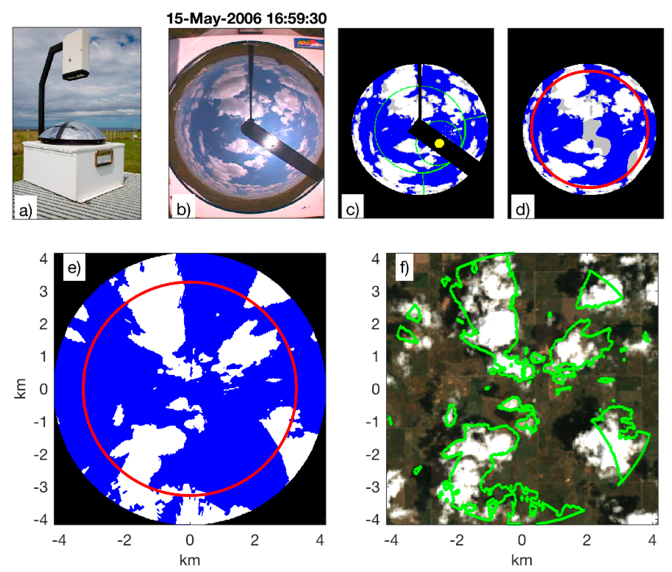
Our approach follows the same three major tasks used in analysis of high-resolution satellite images (e.g., [10,11]): (1) “cloud masking” task, which separates clear-sky and cloudy pixels, (2) “cloud labeling” task, which groups the selected cloudy pixels into individual clouds and (3) “quantitative analysis” task, which provides statistics of influential macrophysical parameters of clouds. Our approach uses the operational processing of the TSI images (Figure 1a–c) for the “cloud masking” task. It should be emphasized that cloud masking errors can propagate to cloud statistics. Two new tasks required prior to the “cloud labeling” task are outlined below: interpolation over image obstructions and projection to planar coordinates.
2.1. Interpolation over Image Obstructions
The TSI cloud mask images are obstructed by the shadowband, camera arm, camera housing and green lines (Figure 1c). These obstructions may divide a large cloud into two or more apparent smaller clouds. To address issues associated with these obstructions, we first expand the existing cloud mask to screen incorrectly classified pixels [15], then use 2D natural interpolation [16] to estimate the pixel mask within the obstructed regions (Figure 1d). The details and evaluation of this processes are described in full in Appendix A.
2.2. Projection of Cloud Mask from Hemispherical to Planar Coordinate System
Each image pixel of a hemispherical TSI image (Figure 1d) represents an approximately equal solid angle of the sky. The image resolution of the TSI was increased on 15 August 2011 from 352 × 288 pixels (original resolution) to 640 × 480 pixels (improved resolution). The area of the sky subtended by a pixel depends on cloud base height (CBH) and pixel zenith angle. We correct for a slight distortion of the TSI mirror [14] and apply the well-known spherical to planar coordinate transformation [17,18].
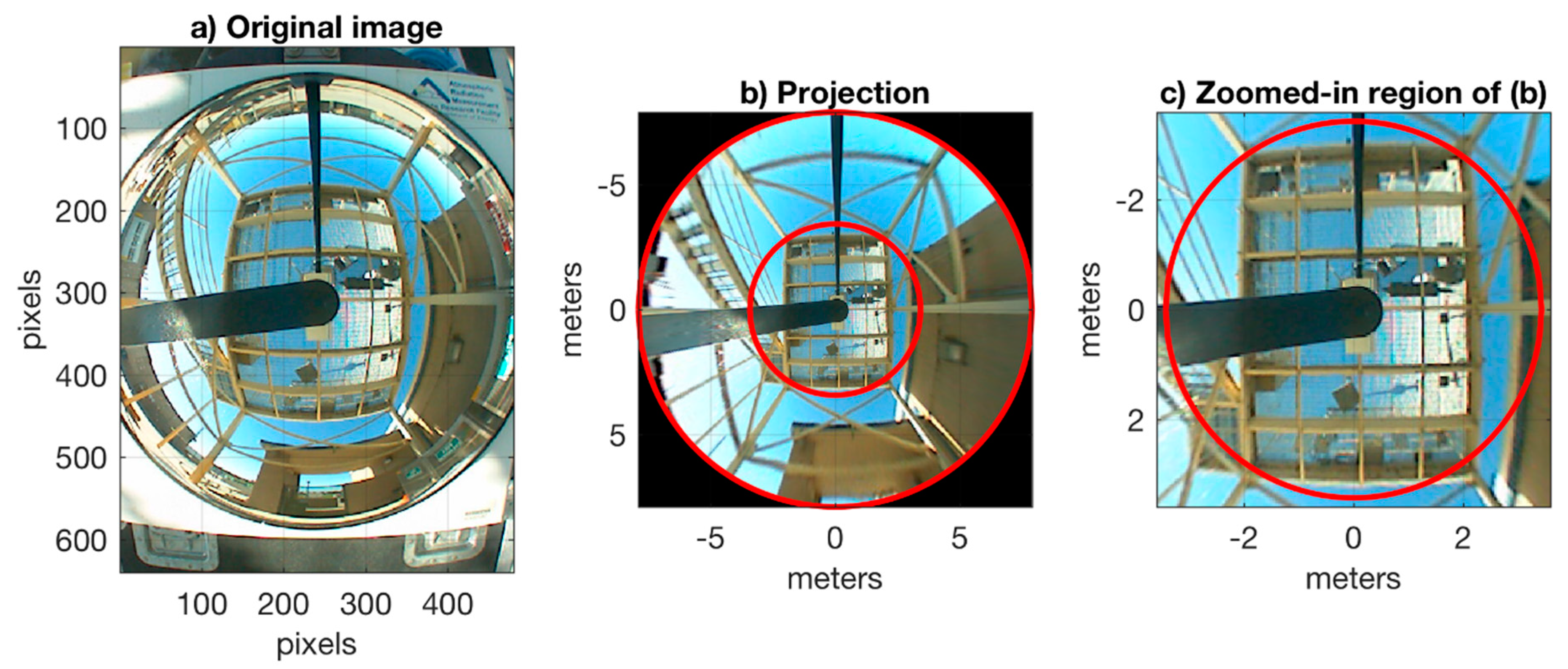
where CBH is derived from lidar measurements (Section 3), θp and φp are the zenith and azimuth angles for each pixel, respectively and xp and yp are resulting pixel coordinates. A single CBH is used for each image transformation, representing all clouds in the scene. This approximation is reasonable given the steady lidar observations of CBH. The transformed pixel coordinates (xp, yp) have irregular spacing. We use triangulation-based linear interpolation to sample the transformed pixel coordinates on a regular grid (Figure 1e). To verify the accuracy of the applied planar coordinate projection, we place a TSI instrument beneath a rectangular platform with known dimension and height (Figure 2) and retrieve platform dimensions using the collected TSI images. We obtain good agreement (~3%) between the known and retrieved dimensions under the control setting. Additional qualitative verification is obtained by overlaying the resulting cloud boundaries obtained from the post-processed TSI cloud mask with the coincident Landsat observation for the five selected dates (Figure 1f and Figure 3).
2.3. Computation of Cloud Areas and the Corresponding CED
Each matrix element in the planar projected cloud mask (Figure 1e) has the same area, allowing for simple calculation of cloud area. Cloudy elements are grouped with an 8-neighbor connectivity criterion, completing the “cloud labeling” task in satellite-based image analysis. The cloud area of the connected region is simply the sum of the element areas [19].
A sequence of TSI images is analyzed to produce statistics on CED, defined as 2√(A/π), similar to the satellite-based “quantitative analysis” task. In our analysis, all cloud areas are retained, including those that are truncated by the 130° FOV circle (Figure 1e). Results of our sensitivity study suggest that 130° FOV is a reasonable trade-off between the anticipated largest sample area (or largest CED) and unwanted influence of cloud side effects (see Appendix B). The cloud truncation at the perimeter limits the observation of large clouds and incorrectly identifies them as smaller clouds. To reduce the influence of this error, we require that clouds truncated at the 130° FOV extend to within a 122° FOV inner region, as determined by a sensitivity study to obtain the best agreement between TSI- and Landsat-derived CED (see Appendix C). This analysis is valid for images with low-to-moderate (<0.4) cloud fraction. The following section highlights the Landsat images and ground-based data required for evaluation of our approach.
3. Data
The integrated dataset includes the ground-based TSI images [20] the best estimate CBH from the ARM Active Remotely Sensed Clouds Locations (ARSCL) cloud product [21], wind speed and direction from the 915-MHz Radar Wind Profiler (RWP) measurements [22] and also high-resolution Landsat images. Hemispheric sky images and corresponding cloud masks are obtained from the TSI Model 880 [23] with enhanced control board and camera installed in 2011. All ground-based data are obtained from the Department of Energy (DOE) Atmospheric Radiation Measurement (ARM) Southern Great Plains (SGP) site, located at 36°36′18″ N, −97°29′6″ E. We use the outlined ground-based and satellite data for selected 5 days with single-layer shallow cumuli to demonstrate the feasibility of our approach (Section 4). What follows is a short description of the collected data and the corresponding instruments.
We select desirable days with single-layer shallow cumuli using multi-year (2004–2017) datasets obtained from the coincident and collocated ground-based and satellite observations. A total of 471 potential days with single-layer shallow cumuli are identified from the Shallow Cumulus Value Added Product [24] using ground-based active and passive remote sensing. The Landsat satellite passes the SGP site infrequently: only once every 16 days at roughly 17:00 UTC (11 a.m. local standard time). We found only 5 days with Landsat images of single-layer shallow cumuli over the SGP site (Figure 4) within the 14-year period (2004–2017) considered here: 2006/05/15 (16:59 UTC), 2007/07/21 (17:01 UTC), 2007/09/23 (17:00 UTC), 2009/05/23 (16:55 UTC) and 2017/06/14 (17:07 UTC). All data described below represent the selected 5 days.A representative CBH and wind vector is determined for each TSI sky image, with 30-s temporal resolution. The ARSCL Value Added Product (VAP) resolves the cloud boundaries with 0.045-km vertical and 10-s temporal resolution [25]. We use a 30-min average of the ARSCL-derived CBH centered at the TSI-capture time as an estimated CBH for the imaged cloud field. The RWP reports the wind vectors with 60-m vertical and 1-h temporal resolution. We use the 1-h average RWP-derived wind vectors closest in time to each TSI image capture time. To reduce noise, we vector average the RWP winds from the three height range gates below, including and above the estimated CBH, ignoring any missing entries, to obtain 1-h averages of wind speed and direction at CBH. It should be mentioned that the vertical span of 180-m is typically less than the standard deviation of the estimated CBH.
The Landsat cloud masks with 0.03-km horizontal resolution identify the majority of shallow cumuli within a 50-km region surrounding the SGP site (Figure 4, top panel). Landsat capture times are within 5 min of 17:00 UTC at SGP and have root-mean-square geodetic accuracy of better than 50 m [26]. We retrieve cloud mask data [27] from the Landsat 5 (L5) and Landsat 8 (L8) missions (datasets courtesy of the US Geological Survey) using the Google Earth Engine online tool (https://code.earthengine.google.com) [28]. Then we combine the cloud masks retrieved for areas located within the 50-km region into a mosaic. The same approach is used for color images. The selected 5 days define different observational conditions with distinct spatial distribution of clouds and cloud fraction ranging by almost an order of magnitude from 0.04 (2007/09/23) to 0.33 (2017/06/14) (see Table 1). Also, we use the RWP-based averages of wind speed and direction at CBH together with the frozen turbulence assumption to estimate size and orientation of the subarea of each Landsat image surrounding the SGP site observed by the TSI (Figure 4, bottom panel). Their widths represent 130° FOV equivalent areas for a given CBH, while their lengths define 1-h equivalent distances for a given wind speed at CBH (Table 1). The main goal of the width and length estimation is to match “case study” areas obtained from Landsat (instantaneous snapshot) and TSI (1-h averaging) observations. Such area matching is required for comparing the basis statistics of the TSI- and Landsat-derived CEDs (Section 4). We determine the Landsat-derived CEDs similarly to those from TSI data (Section 2), except that Landsat-derived cloud area is never truncated due to FOV limitations (we censor one erroneous cloud on 14 June 2017, Figure 4b). Landsat cloudy pixels located within and outside of the red rectangle (Figure 4, bottom panel) are considered part of a given cloud (navy shaded clouds in Figure 4).
4. Results
Prior to comparing CED statistics obtained from the Landsat and TSI observations, we outline challenges and solutions to a balanced comparison. First, the satellite and ground-based observations likely have different sensitivities to cloud optical and geometrical properties, resulting in different cloud areas. Second, while an apples-to-apples comparison on a single coincident capture (see Figure 3) can be made, a comparison of cloud field statistics from the TSI and Landsat image requires employing the frozen turbulence assumption. In other words, we assume that the cloud field is evolving slowly enough that the single instantaneous Landsat capture is comparable to the TSI-observations acquired over 1-h period. This assumption may break down when the cloud field is non-stationary over the 1-h averaging period. Thus, the Landsat and TSI cloud masks may represent different cloud populations. Third, the TSI CEDs represent both truncated and non-truncated clouds, while the Landsat CEDs define non-truncated clouds only. As a result, TSI CEDs likely underestimate Landsat CEDs and this underestimation can be size-dependent. Fourth, the TSI can view cloud sides at large zenith angles, sometimes resulting in merged clouds. Finally, the TSI image interpolation over the shadowband region may introduce additional errors.
To quantify the combined impact of the sampling strategy (second challenge) and cloud truncation (third challenge) on the level of agreement between the TSI and Landsat CEDs, we introduce simulated TSI-like observations of the Landsat image. The TSI-like observations consist of 120 circular instances of the Landsat image, captured with TSI-equivalent 130° FOV for a 1-h averaging period along the wind direction, simulating a 30-s temporal resolution within the Landsat subarea (See Figure A3). The TSI-like observations observe each cloud multiple times, truncate clouds at the 130° FOV and retain only truncated clouds that extend to less than 122° FOV, as does the TSI.
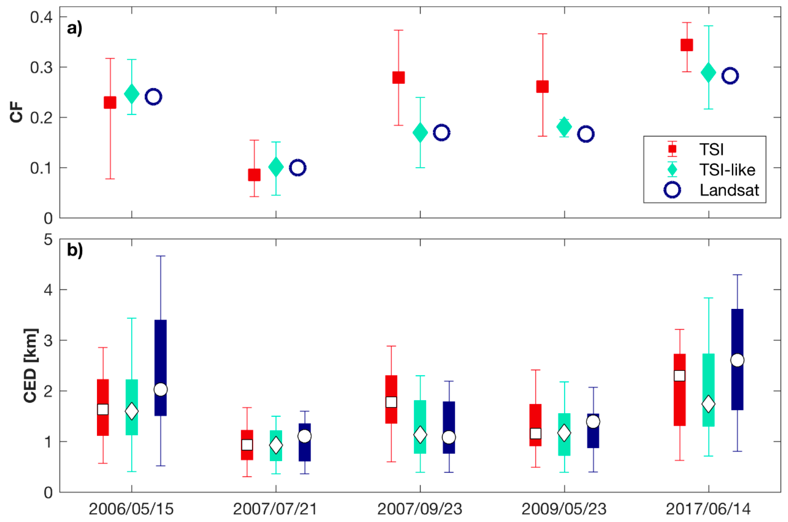
The cloud fraction (CF) obtained from the TSI and TSI-like simulator reveal differences in spatial and temporal sampling (Figure 5a). The 15-min TSI average (red bars) indicates temporal variability over the 1-h observation period, while the TSI-like 15-min average indicates spatial variability within the Landsat subarea (green bars). The Landsat subarea CF (blue circles) and TSI-like 1-h average (green diamonds) show nearly perfect agreement, as expected. The TSI CF indicates non-stationary cloud fields on 2006/05/15, 2007/09/23 and 2009/05/23. The TSI 1-h and Landsat subarea averages (symbols) agree to within 10 percentage points on the two stationary days and 2006/05/15 due to a steady increase in CF over the 1-h averaging period. On the two remaining days: (1) 2007/09/23 contains an inaccurate TSI cloud mask caused by sun glare (see Figure 5b) as well as an inhomogeneous and non-stationary cloud field and (2) 2009/05/23 has a non-stationary cloud field.
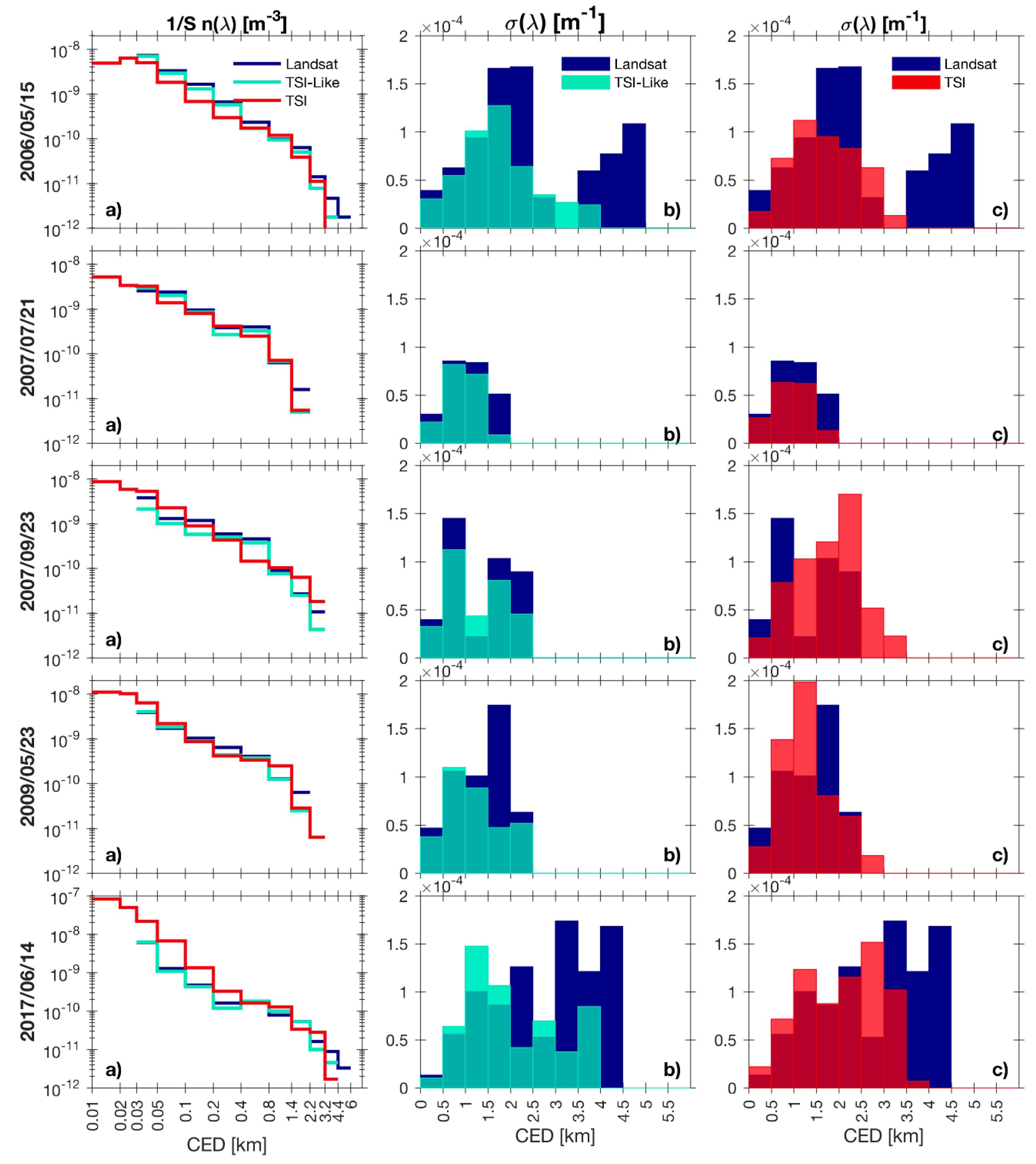
Statistical comparisons of the cloud area distributions measured by the TSI and Landsat are made following the approaches introduced previously by others. In particular, the normalized cloud size distribution n(λ) is defined as
where λ is the CED, S is the total area of sky observed and N is the number of clouds observed per unit area. The normalized cloud size distribution (Figure 6a) shows that the smallest clouds are most numerous, consistent with many other studies for example, [29]. The TSI resolves a wide range of cloud sizes from 0.01 km to about 3.5 km (see Appendix D for lower limit and Appendix C for upper limit), while Landsat has no upper bound on cloud size. The cloud size distribution n(λ) commonly extends over multiple decades in scale (0.01–10 km for shallow cumulus) [1], which does not easily suggest a central or mean cloud size.
On the other hand, the cloud cover density is defined as [7]
where a(λ) is the cloud area π(λ/2)2. Note that σ(λ) commonly has peaked distributional shape that can be described using a summary statistic of cloud size. The cloud cover density represents the contribution of each CED to cloud cover, such that the integral of σ(λ) over λ results in the cloud fraction. We draw two cloud size statistics from the cloud cover density: the characteristic size λc is the expected value of the cloud cover density [7]
and the median of the cloud cover density, L50, describes the cloud size for which half of the cloud fraction is derived from clouds smaller than L50 [29].
The median L50 and other percentiles of the cloud cover density σ(λ) (Equation (3)) illustrate differences in CED obtained from these three approaches (Figure 5b). The three approaches TSI, TSI-like and Landsat show mutual agreement when there is a high-quality TSI mask and Landsat L50 is less than 2 km (2007/07/21 and 2009/05/23). The TSI and TSI-like interquartile ranges show excellent agreement on all days with correct TSI mask (Figure 5b, red and green bars). The percent difference of TSI compared to TSI-like L50 ranges from −2% (2009/05/23) to +32% (2017/06/14), with a mean absolute percent difference of 9%. Similarly, the percent difference of TSI to TSI-like λc ranges from −2% to 8% with a mean absolute difference of 3%. This error is due to sensor differences, inclusion of cloud sides and interpolation and is considered secondary to the effect of cloud truncation and spatio-temporal differences (Appendix B discusses the sensitivity of CED on FOV). The cloud cover densities (Figure 6b,c, red and green bars) further demonstrate this close agreement. More generally, comparison of Landsat λc from clouds that appear within the TSI field of view (but are not sampled as in the TSI-like) with TSI returns a mean absolute percent difference of 7%. All central cloud sizes are presented in Table 2.
The full Landsat cloud sizes, which are never truncated, extend beyond the 130° FOV (blue clouds in Figure 4). Consequently, both TSI and TSI-like cloud cover densities fail to resolve clouds larger than about 3.5 km (Figure 6b,c; see 2006/05/15 and 2017/06/14). Not only are these clouds outside of the TSI field of view but the sinewy connections in the Landsat image suggest that closely-spaced clouds may be falsely merged by Landsat. One such example in the northeast region of Figure 4a, 2017/06/14, was omitted from the analysis for this reason. The radius of the circular sky observed in a single TSI image (Table 1) is comparable to 3.5 km, making this a sensible upper bound. We generalize this result to expect an upper bound of resolvable cloud size at the radius of the projected image, which is roughly two times the CBH for a 130° FOV. The overall percent error in L50, taken as the difference over the Landsat value, is (19%, 16%, 17% and 12%) for the four days with high-quality TSI mask, in chronological order, for a mean error of 16% (Table 2). This error is biased low due primarily to the truncation of clouds at the 130° FOV and is evaluated only from cloud fields with small-to-moderate (<0.4) cloud fraction.
5. Conclusions
We develop a novel approach that resolves cloud area distributions of single-layer shallow cumuli from ground-based observations and estimates cloud equivalent diameter (CED) over a wide range of cloud sizes (about 0.01–3.5 km) with high temporal resolution (30 s). Our approach is computationally inexpensive and relies on sky images obtained from Total Sky Imager (TSI) and complementary information on cloud base height provided by lidar measurements. We illustrate performance of our approach using coincident 0.03-km Landsat cloud masks obtained for five periods with single-layer shallow cumuli over the Atmospheric Radiation Measurement (ARM) Southern Great Plains (SGP) site. We demonstrate that TSI and Landsat CEDs are in good (~7%) agreement for clouds that fall within the TSI field of view (FOV) limit (~3.5 km) and noticeable (~16%) underestimation of the TSI CEDs is due to large clouds that extend beyond the TSI FOV limit. We demonstrate that a similar sampling strategy of the TSI and Landsat data results in strong (~3%) agreement, indicating that the limited FOV is a primary influence on the comparison, while other factors associated with visibility of cloud sides, 2D interpolation over image obstructions and different sensitivities of the ground-based and satellite sensors to cloud properties are secondary. An extension of this approach could involve tracking clouds as they pass through the TSI FOV, enabling observation of larger clouds along the wind direction. Since many sites world-wide deploy sky imagers, including DOE ARM fixed and mobile facilities, our approach can be applicable to data collected at different locations and times. Our approach provides previously unavailable datasets that can contribute to improved understanding of the diurnal cycle of cumulus convection at various temporal and spatial scales and can offer a unique opportunity to carefully evaluate and improve large-eddy simulation (LES) results of shallow cumuli cloud size and cloud fraction [30,31,32].
Author Contributions
Conceptualization, J.M.K. and E.K.; Formal Analysis, J.M.K.; Validation, E.A.R.; Writing-Original Draft Preparation, J.M.K., E.K. and E.A.R..; Writing-Review & Editing C.N.L., L.D.R., L.K.B. and V.R.M.; Methodology, J.M.K., E.K., E.A.R., L.D.R., C.N.L. and L.K.B.; Data Curation, V.R.M., L.D.R. and C.N.L.; Resources, L.D.R.
Funding
This research was supported by the U.S. Department of Energy’s Atmospheric System Research Grant DE-SC0016084 and KP1701000/57131 and MJ Murdock Charitable Trust Grant 320-1685. The Pacific Northwest National Laboratory is operated by Battelle Memorial Institute under contract DE-AC06-76RLO 1830.
Conflicts of Interest
The authors declare no conflict of interest. The funders had no role in the design of the study; in the collection, analyses, or interpretation of data; in the writing of the manuscript and in the decision to publish the results.
Appendix A. Two-Dimensional Interpolation over Image Obstructions
Image interpolation is sensitive to the cloud mask of pixels adjacent to the non-sky regions. However, these pixels are often erroneously classified due to differences between the masked and true locations of the shadowband, camera box and camera arm in the TSI images. It is essential to remove erroneous pixels from the vicinity of the image obstructions prior to interpolation.
An expanded image mask is constructed for each image prior to interpolation. Note that the TSI images have variable resolution (or number of pixels): low-resolution (352 × 288 pixels) images prior to August 2011 and high-resolution (480 × 640 pixels) thereafter. The processing steps described below differ slightly for the low- and high-resolution images. The first step is to increase (25%) uniformly an area covered by the shadowband, which is oriented along the solar azimuth angle from the center of sky image. The second step is to identify pixels that visibly correspond to camera arm or housing that were not previously masked. For our identification, we use thresholds on the HSV (hue, saturation, value) transformation of the sky image [33] as follows: H < 0.3, S > 0.95, or V < 0.45 within a vicinity of 25 pixels of the camera arm or housing. The third step is to create a continuous mask with no internal gaps using the morphological flood-fill operation [19] and remove non-connected masked regions with small sizes (3 × 3 pixels or smaller) using morphological image opening. Finally, we expand the entire image mask by 2 pixels using morphological image dilation. Table A1 summarizes these adjustments for both low and high-resolution images.
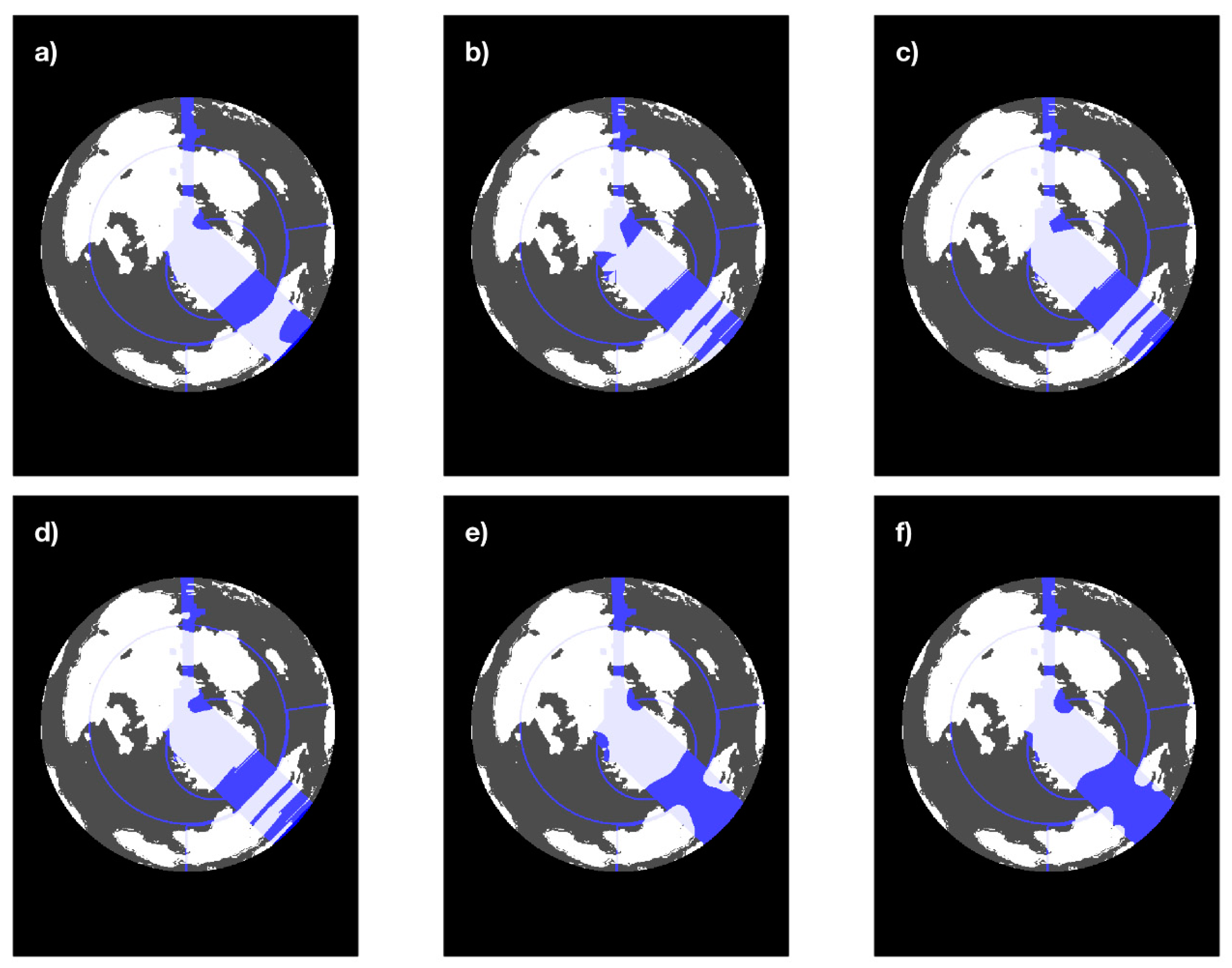
A two-dimensional (2D) image interpolation is used to estimate number of clear-sky and cloudy pixels in non-sky regions within the 160° field of view (FOV) of the TSI decision image. Six interpolation schemes are tested: nearest neighbor, linear, cubic and natural interpolation [16] using MATLAB’s grid data function and the Laplacian (∇2) interpolation motivated by the heat diffusion equation [34,35]. A sample interpolated image is presented in Figure A1. Visual comparison of the interpolated images show that the natural interpolation and eight-neighbor average interpolation produce the most reasonable contours, while the nearest neighbor, linear and cubic interpolation are poor reconstructions of occluded clouds.

Table A1.
Expansion of the non-sky regions of the TSI cloud mask prior to image interpolation.
| Mask Parameter | Resolution | Default Cloud Mask | Adjusted |
|---|---|---|---|
| Image width | low | 125 pixels | n/a |
| high | 207 pixels | n/a | |
| Shadowband width | low | 34 pixels | 42 pixels |
| high | 60 pixels | 76 pixels | |
| Camera arm width | low | 7 pixels | Up to 10 pixels * |
| high | 14 pixels | Up to 25 pixels * | |
| Camera box size | low | varies | Up to 25 pixels * |
| high | varies | Up to 25 pixels * |
* The camera arm and camera box regions are expanded based on the applied thresholds, as described above.
Figure A1.
TSI cloud mask for a sample image with 160° FOV captured on 14 June 2017 17:29:30. The cloud mask includes interpolated image region with blue shading using (a) natural interpolation, (b) nearest neighbor, (c) linear interpolation, (d) cubic interpolation, (e) 8-neighbor average, (f) Laplacian ∇2 interpolation. Interpolation over the camera arm (vertical line to the top of the image) and green lines (Figure 1c) appears robust. Artifacts introduced in the shadowband region (diagonal line to the lower right) depend on interpolation method used.

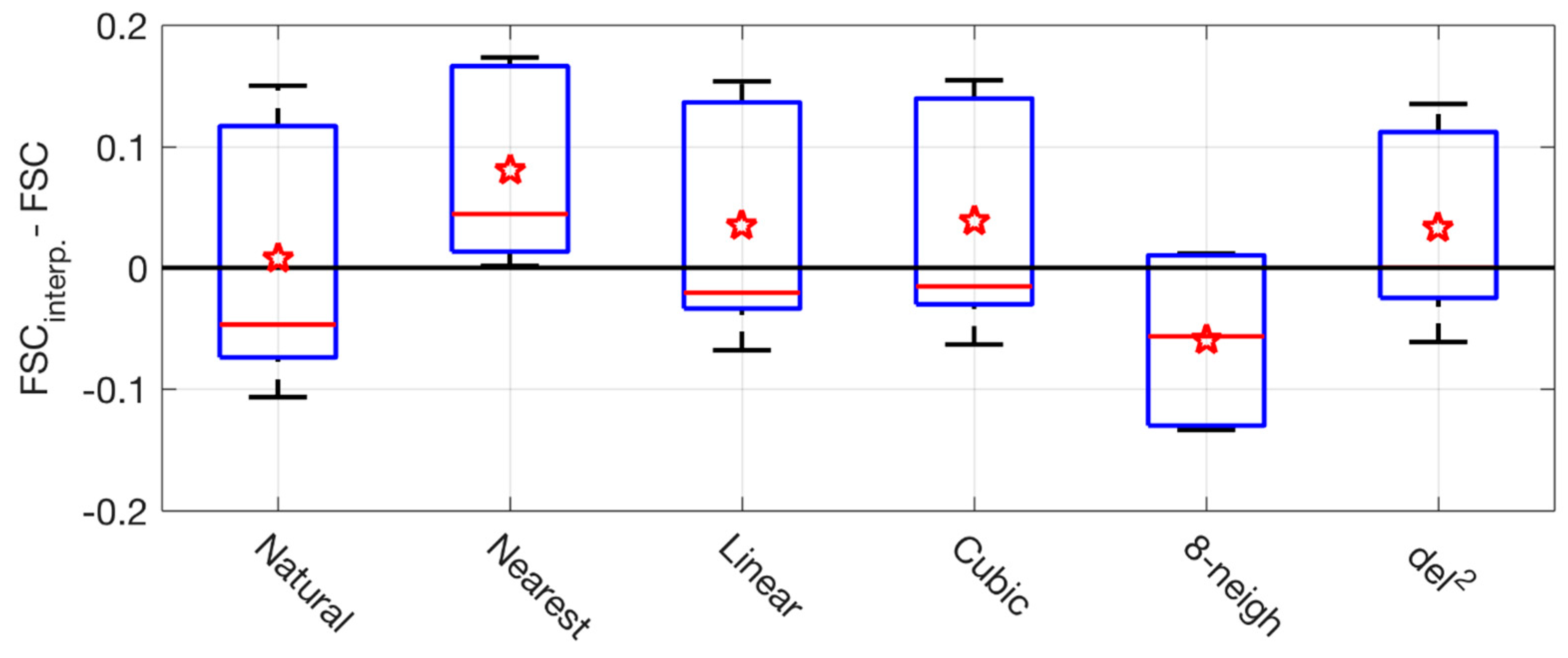
To further assess the quality of the interpolation schemes, we compare fractional sky coverage (FSC) calculated over two disjoint regions: (1) the interpolated region only and (2) the original (non-interpolated) cloud mask (Figure 1c). The FSC is calculated as the ratio of the number of opaque-cloudy pixels to the total number of pixels. The comparison tests an assumption that values of FSC calculated for the interpolated and the non-interpolated regions should be comparable over sufficient averaging time. To take into account for the small size of the interpolated region, we compare 60-min mean values of the calculated FSC. Results in Figure A2 show that the natural interpolation produces the smallest difference between the mean values calculated for the interpolated and the non-interpolated regions.
We select the natural interpolation as the best interpolation scheme based on visual appearance of the interpolated region (Figure A1) and agreement of the reconstructed fractional sky coverage (Figure A2). It is clear from comparison with the Landsat images (Figure 3) that cloud boundaries are reconstructed reasonably well for the camera arm and green line regions and sometimes poorly for the shadowband region. The FSC comparison suggests that interpolation introduces a random error in cloud identification within the observational precision of the TSI of 10 percentage points (FSC ± 0.1).
Figure A2.
Distributions of the difference between fractional sky coverage (FSC) calculated for the interpolated and non-interpolated regions. One hour of TSI images centered on the five Landsat images are analyzed for different interpolation schemes. The 60-min average “opaque-cloud-only” FSCs are obtained for the interpolated region only (FSCinterpolated) and the original cloud mask only (FSC). Red star and red line show the mean and median values for the difference between FSCs calculated for the interpolated and original images, respectively. Boxes and whiskers define percentiles (25th and 75th) and minimum/maximum values, respectively.

Appendix B. Sensitivity Study of Maximum Field of View
The TSI cloud observations routinely truncate clouds at the outer perimeter of the projected image field of view (FOV). This section addresses the following questions:
- How sensitive is the TSI CED product to the maximum FOV?
- How does the maximum FOV influence agreement between TSI-derived and Landsat-derived CED?
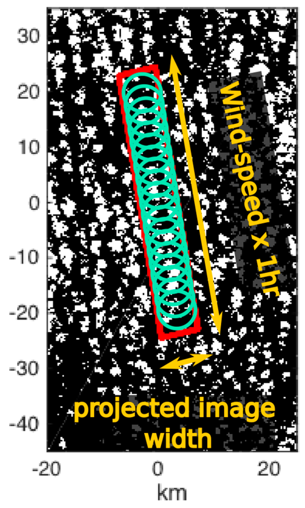
To isolate the cloud truncation effect, we introduce a TSI-like sampling simulation using the Landsat images. Similar to the TSI observations, the simulation samples the cloud field within a given FOV every 30 s (Figure A3) assuming that the static cloud field moves with the wind over the SGP site. In contrast to the TSI observations, the simulation uses the Landsat images. The TSI-like product differs from the Landsat product due to two main factors: (1) multiple observations of the same clouds (Figure A3) and (2) cloud truncation at the outer FOV. Whereas the TSI-like product differs from the TSI product due to three main factors: (1) different sensitivity of the Landsat and TSI instruments to the cloud properties, (2) ignoring the impact of cloud sides at large zenith angles and (3) ignoring the temporal evolution of the cloud field during the averaging period.
Comparison of the TSI-like observations with non-truncated Landsat observations highlights the effect of FOV truncation without introducing other sources of error. The right two columns of Table 1 show that the number of clouds observed by the TSI. This number is 9 to 53 times larger than the number of clouds observed within the Landsat subarea for these five cases. This suggests that there is a distribution of residency times for clouds remaining within the TSI FOV. The difference between TSI-like and TSI number of clouds is primarily due to sensor differences and can be affected by non-stationary cloud fields.
Figure A3.
Cartoon of generation of TSI-like images sampling the cloud mask from Landsat image captured on 15 May 2006, 16:59 UTC. Red box indicates the Landsat subarea observed by the TSI over a 1-h analysis period with a 130° FOV with SGP site at the origin. Green circles indicate 30-s simulated TSI-like observations as the frozen cloud field moves overhead, actual simulation uses 120 green circles. The TSI-like clouds are truncated at the 130°-FOV circle, whereas the Landsat cloud sizes are not truncated.

Figure A4.
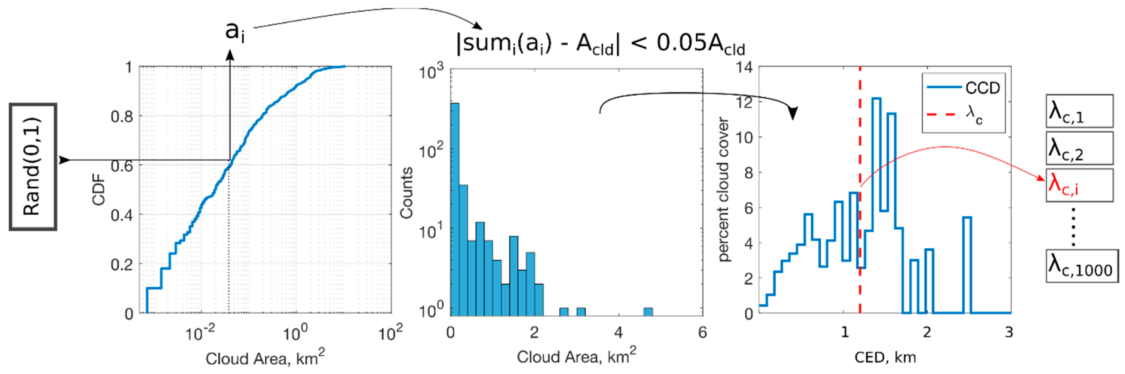
Cartoon of inverse-sampling of TSI or TSI-like cloud size to derive the ensemble mean and confidence interval of characteristic cloud size (λc). Uniformly distributed random numbers on (0,1) are used to draw cloud areas (ai) from the TSI or TSI-like CDF. The stopping criteria is set such that the sum of the ai is equal to the total cloud area (Acld) from the Landsat subarea within a 5% tolerance. The normalized cloud cover density (CCD) is then computed and characteristic size, λc, is calculated. This inverse sampling routine is repeated until 1000 values of λc are obtained. The mean and 95% confidence interval (CI) of λc are reported and compared to the Landsat subarea (Figure A5b,c).
Figure A4.
Cartoon of inverse-sampling of TSI or TSI-like cloud size to derive the ensemble mean and confidence interval of characteristic cloud size (λc). Uniformly distributed random numbers on (0,1) are used to draw cloud areas (ai) from the TSI or TSI-like CDF. The stopping criteria is set such that the sum of the ai is equal to the total cloud area (Acld) from the Landsat subarea within a 5% tolerance. The normalized cloud cover density (CCD) is then computed and characteristic size, λc, is calculated. This inverse sampling routine is repeated until 1000 values of λc are obtained. The mean and 95% confidence interval (CI) of λc are reported and compared to the Landsat subarea (Figure A5b,c).

The summary cloud size statistic employed to evaluate sensitivity to maximum FOV is the characteristic cloud size λc (Equation (3)). The true distribution of cloud sizes is generally not known for a given TSI observation, so statistical inference is needed to relate the true distribution to the observed TSI CED. We use the approach of inverse sampling from the cumulative distribution function of TSI and TSI-like cloud areas, depicted schematically in Figure A4. The stopping criteria for the inverse sample is set such that the sum of the cloud areas in the sample is equal to the sum of the cloud areas in the Landsat subarea region for each FOV employed. For the TSI-like results, the total cloud area is calculated from the sum of all clouds within and touching the swath boundary (not truncated). For real TSI results, we use the mean TSI cloud fraction times the swath area to determine total cloud amount for each FOV employed. We generate 1000- bootstrapped populations of cloud area for each of the 5 satellite dates using FOVs of 100, 110, 120 and 130. We determine from the visual inspection of the TSI images that a 140° FOV is beyond the sensor’s capacity (see Figure 1).
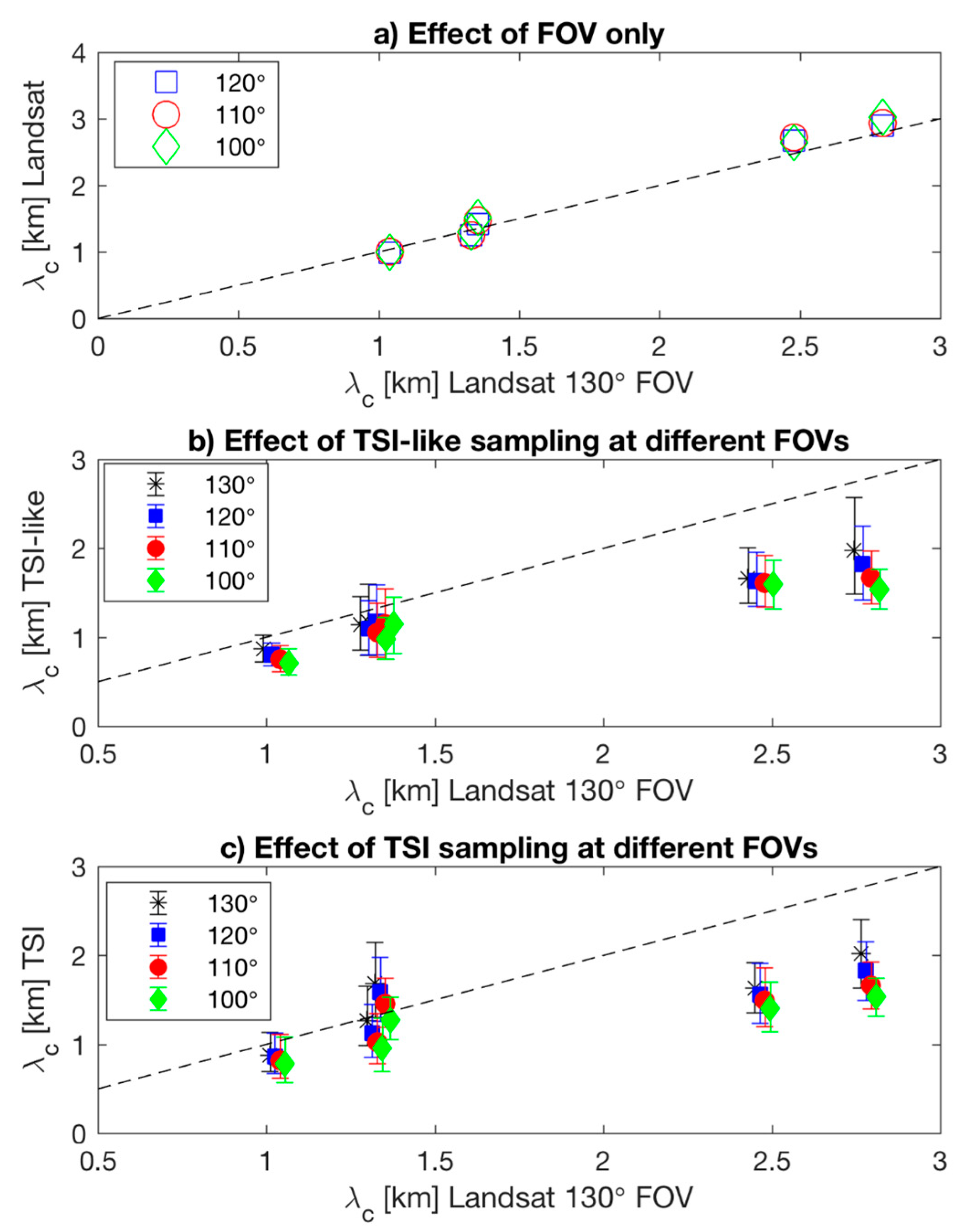
We calculate a mean and 95% confidence intervals from the 1000 bootstrapped characteristic cloud sizes, λc. Since the Landsat CED includes the entire cloud contours, λc from Landsat images does not depend strongly on the maximum FOV (Figure A5a). The mean λc from the TSI-like simulator is always less than or equal to the Landsat λc obtained for the full cloud contours (Figure A5b). As the maximum FOV is decreased from 130° to 100°, the mean and 95% confidence intervals of the mean decrease. The largest CEDs obtained for 2017/06/14 show the most dramatic decline, which is expected: the largest clouds will be the most affected by truncation at the edge and λc is sensitive to the few large clouds in the sample. Furthermore, the 95% confidence intervals decrease with decreasing maximum FOV, suggesting that the population is being significantly altered. The different rates of decreasing λc with decreasing FOV for the five days depends upon the location of clouds within the TSI-like FOV: clouds that pass more directly overhead are less sensitive to truncation by the outer FOV. Conversely, a large cloud that does not pass overhead may be perpetually truncated.
Figure A5.
(a) Effect of maximum field of view (FOV) on characteristic cloud size (λc) observed from the Landsat subarea. All clouds touching the FOV are included as whole. Dashed line is 1:1. (b) Mean and 95% confidence interval of λc from 1000 simulated cloud fields drawn from simulated TSI-like cumulative distribution functions (see Figure A4). The TSI-like data drawn from four different FOVs are compared to 130° FOV Landsat data with a slight horizontal offset for visualization. (c) Same as Figure A5b, except using the real TSI data.

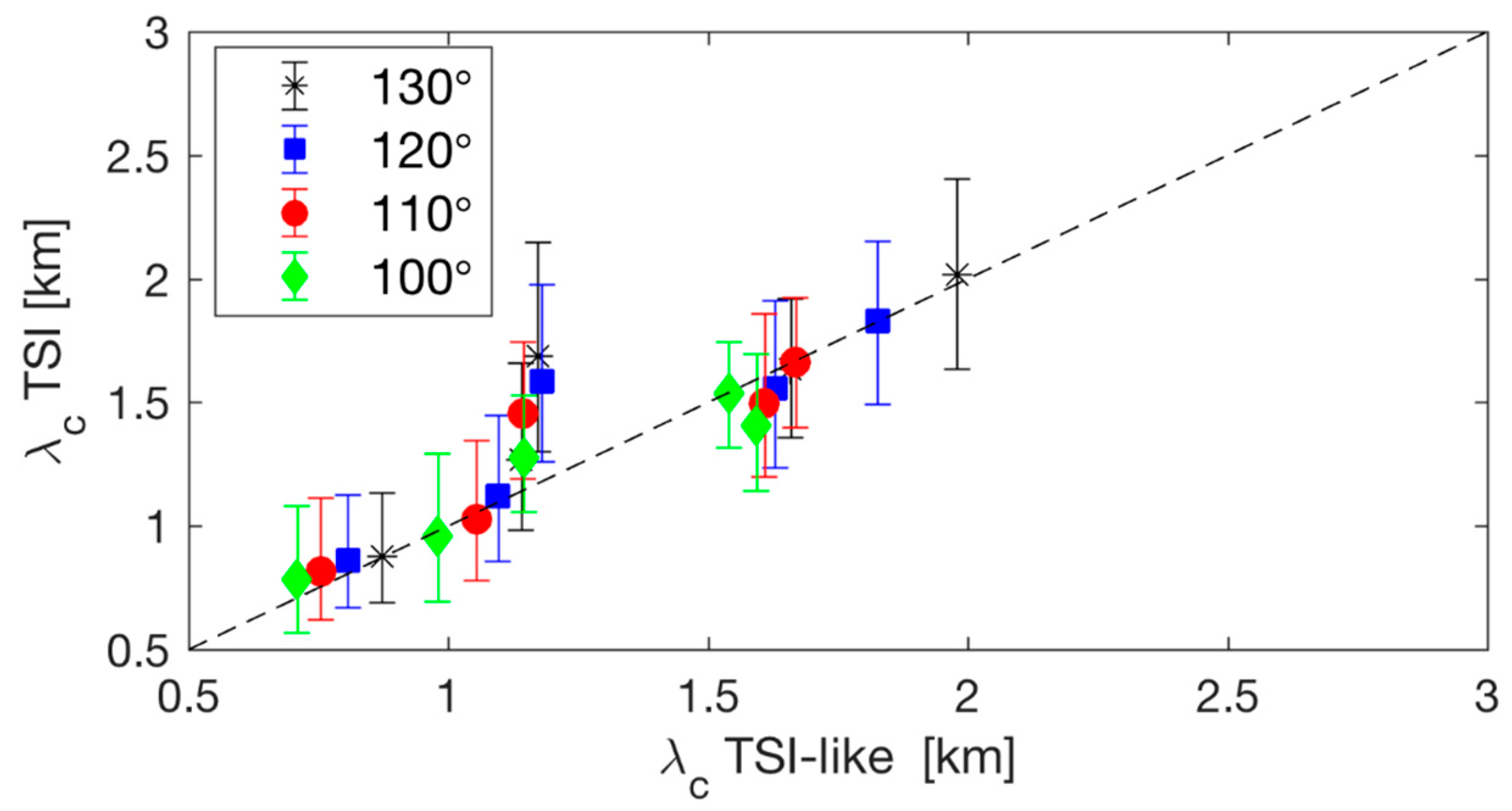
The effect of the maximum FOV on the TSI CED shows a similar trend of decreasing cloud size with decreasing maximum FOV (Figure A5c). The agreement between λc for TSI and TSI-like sampling is striking (Figure A6). In some cases, the TSI results show a slightly enhanced λc for 130° FOV and thus indicates that viewing cloud sides and merging clouds are increasing the CED more than expected from the expanded FOV. The obtained strong agreement suggests: (1) the maximum FOV is the dominant limitation of the TSI CED product, (2) a 130° maximum FOV only marginally includes larger clouds due to cloud sides and merging. Note that the maximum cloud fraction for these five days is 0.33 (Table 1). The sensitivity study for the TSI CED product cannot be considered valid for large (>0.4) cloud fractions where the cloud merging may play a greater role.
Figure A6.
Comparison of TSI to TSI-like characteristic cloud size (λc) from 1000 simulated cloud fields drawn from the cumulative distribution functions. Symbols indicate ensemble mean λc and error bars depict 95% confidence intervals for TSI. The maximum FOV is set to 130° (black asterisk), 120° (blue square), 110° (red circle) and 100° (green diamond). Differences between the TSI and TSI-like results are due to several factors, such as sensor differences (including sun glare), inclusion of cloud sides, evolution of cloud fields over the 1-h analysis period and the 2D interpolation.

We conclude by revisiting our two guiding questions: (1) How sensitive is the TSI CED product to the maximum FOV? The characteristic cloud size decreases as the maximum FOV decreases, due to systematic truncation of the largest clouds. The dependence is greatest for large clouds that do not pass directly overhead and is least for small cloud fields. (2) How does the maximum FOV influence agreement between TSI-derived and Landsat-derived CED? The maximum FOV and resulting cloud truncation is the dominant source of difference between Landsat and TSI-derived CED. This is concluded from the strong agreement between TSI-like and TSI observations and strong dependence upon maximum FOV (Figure A6). The second greatest uncertainty is due to sensor differences, including sun glare errors in the cloud mask, as evidenced on 2007/09/23, when the 130° FOV TSI-derived CED shows the greatest difference from the 130° TSI-like CED from Landsat data. Other possible sources of difference include interpolation uncertainty and inclusion of cloud sides.
Appendix C. Incomplete Viewing of Clouds (Truncation)
The text in Appendix B is devoted to the maximum field of view but does not consider the impact of clouds partially within the field of view. In Appendix A, we discussed that the TSI sampling results in multiple measurements of clouds passing through the field of view. The best measurement of a cloud’s area would then be when the cloud has passed completely within the FOV, whereas the cloud area is underestimated when it is partially within the FOV. However, if all clouds touching the maximum FOV were excluded, then almost all large clouds (CED > 3 km) would likely be censored resulting in a drastic underestimation of the largest clouds. In this section, a sensitivity analysis is performed to determine which of the truncated clouds are reasonable to retain to achieve the best estimate of the true cloud distribution.
Using Landsat and TSI-like data, we generate a composite case combining all 5 case days into one dataset to determine an additional inner FOV threshold for which to exclude clouds that are touching the maximum FOV. All the Landsat (non-truncated) clouds are labeled with an index, these indices allow cloud tracking in the TSI-like data set so that each instance of a unique Landsat cloud is recorded as it passing through the TSI-like FOV.
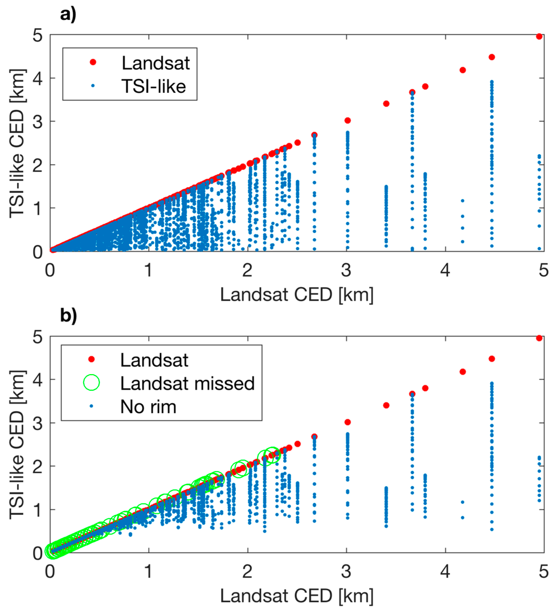
Figure A7a shows the composite case where each measurement of CED from TSI-like is plotted against the “true” Landsat cloud area. For example, the Landsat cloud with CED of ~5 km is measured 9 times (blue dots) in the TSI-like sampling. In each of the 9 simulated TSI images in which this cloud appears, the cloud area is truncated different amounts. In Figure A7 all blue dots below the 1:1 diagonal (red dots are unique Landsat clouds) are truncated at the 130° FOV. In Figure A7b a FOV cut-off of 122° is employed, where clouds outside of 122° and touching the 130° FOV are censored. Removal of these so called “rim clouds” (owing to their location at the edge of the FOV) improves the estimate of cloud area for the smallest sizes (very few points below the 1:1 diagonal for CED < 1 km). It also removes the poorest measurements of the large clouds.
Figure A7.
The effect of cloud truncation by maximum FOV and a possible mediating solution. All information is derived from Landsat images. The abscissa shows the full (non-truncated) CED and the ordinate shows multiple observations of each cloud with TSI-like truncation. Clouds from all five Landsat subareas are included as a composite, omitting a single massively merged Landsat cloud from 2017/06/14. (a) All observations. 10,101 TSI-like clouds are shown (blue dots), of these 3252 have areas less than the original Landsat, (b) The 2076 observations of “rim” clouds have been removed. “Rim” clouds are truncated at a FOV of 130° and exist outside of a 122° FOV. This composite includes 609 unique clouds from the Landsat swath. Removing the “rim” clouds results in censorship of 67 clouds (green circles).

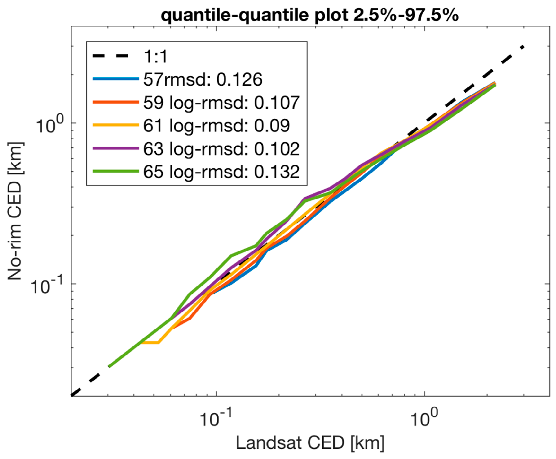
Figure A8 shows how the 122° FOV inner threshold was determined. The root-mean-squared difference (RMSD) between the log-transformed quantiles drawn from the true Landsat distribution and the TSI-like distribution was used as a selection criterion. The log transformation was used to place more weight on the small and medium sized CED rather than the largest CED, which are expected to be underestimated by the TSI. The inner FOV cut-off was chosen as the minimum of the RMSD for the composite case (see Figure A8).
Figure A8.
Quantile-quantile plot comparing 2.5th to 97.5th quantiles of TSI-like to full Landsat CED distributions drawn from cloud size distributions (Equation (2)). Colored lines indicate the minimum zenith angle that a cloud must subtend to be included. A minimum zenith angle of 65° (green) includes all clouds and shows that the TSI-like over-estimates clouds under 0.6 km. Minimum zenith angles of 63° (purple) and 61° (yellow) show good agreement for clouds with CED < 1 km, while minimum zenith angles of 59° (red) and 57° (blue) underestimate clouds under 0.6 km. All TSI-like observations underestimate large clouds with CED > 0.8 km; this cannot be improved by removing rim clouds. The log-root mean squared difference is computed for each population, indicating that 61° shows the best agreement.

Appendix D. Spatial Resolution of Projected Images
The minimum observable CED from the TSI is determined by the spatial resolution of the planar projected TSI image. It is important to understand limitations on the resolution and spatial domain of the earth projected images for interpretation of the cloud size product. The areal representation of a pixel depends upon its zenith angle θp and the cloud base height. Urquhart et al. [36] present a discussion of image resolution for equi-solid angle cameras, such as the TSI. The area of a pixel projected to a plane parallel to the ground can be expressed
where α is the pixel field of view (half-angle). For an equi-solid angle lens, α should be constant for all pixels. If there are npix pixels in the 180° FOV sky region of the image, then each pixel has a solid angle of Ωpix = 2π/npix. Solid angles relate to half-angles α like Ωpix = 2π (1 − cos α). Images prior to (after) August 2011 contain approximately 57,300 (176,000) pixels within the entire 180° FOV. As a result, the corresponding pixel half-angle α is 0.34° (0.19°). Equation (A1) then suggests that for CBH = 1500 m, the ground dimension () of a pixel with zenith angle of θp = {0°, 20°, 40°, 60°, 70°} is {16 m, 17 m, 23 m, 44 m, 79 m} for image prior to August 2011 and {9 m, 10 m, 13 m, 25 m, 45 m} after. The total areal extent observed by a single TSI image depends strongly upon the maximum zenith angle used for the image projection, θmax, such that the diameter of the projected image is given by
After mapping each TSI pixel to planar coordinates (Equation (1)), the planar image is reconstructed using triangulation-based linear interpolation to a square linear grid with resolution D/(2nw), where nw is the original image width: 288 and 480 pixels before and after August 2011, respectively. Thus, for CBH = 1500 m and for maximum zenith angle θmax = {50°, 60°, 70°} the gridded earth-projected image has a gridded resolution of {6 m, 9 m, 15 m} prior to 2011 and {7.4 m, 11 m, 17 m} after 2011 respectively. The spatial resolution of pixels with the smallest zenith angles are retained in the mapping.
References
- Benner, T.C.; Curry, J.A. Characteristics of small tropical cumulus clouds and their impact on the environment. J. Geophys. Res. 1998, 103, 28753–28767. [Google Scholar] [CrossRef] [Green Version]
- Koren, I.; Oreopoulos, L.; Feingold, G.; Remer, L.A.; Altaratz, O. How small is a small cloud? Atmos. Chem. Phys. 2008, 8, 3855–3864. [Google Scholar] [CrossRef] [Green Version]
- Berg, L.K.; Kassianov, E.I. Temporal variability of fair-weather cumulus statistics at the ACRF SGP site. J. Clim. 2008, 21, 3344–3358. [Google Scholar] [CrossRef]
- Berg, L.K.; Kassianov, E.I.; Long, C.N.; Mills, D.L. Surface summertime radiative forcing by shallow cumuli at the Atmospheric Radiation Measurement Southern Great Plains site. J. Geophys. Res. 2011, 116, D01202. [Google Scholar] [CrossRef]
- Kivalov, S.N.; Fitzjarrald, D.R. Quantifying and modelling the effect of cloud shadows on the surface irradiance at tropical and midlatitude forests. Bound.-Lay. Meteorol. 2018, 166, 165–198. [Google Scholar] [CrossRef]
- Chandra, A.S.; Kollias, P.; Albrecht, B.A. Multiyear summertime observations of daytime fair-weather cumuli at the ARM Southern Great Plains Facility. J. Clim. 2013, 26, 10031–10050. [Google Scholar] [CrossRef]
- Rodts, S.M.A.; Duynkerke, P.G.; Jonker, H.J.J. Size distributions and dynamical properties of shallow cumulus clouds from aircraft observations and satellite data. J. Atmos. Sci. 2003, 60, 1895–1912. [Google Scholar] [CrossRef]
- Jiang, H.; Feingold, G.; Jonsson, H.H.; Lu, M.; Chuang, P.Y.; Flagan, R.C.; Seinfeld, J.H. Statistical comparison of properties of simulated and observed cumulus clouds in the vicinity of Houston during the Gulf of Mexico Atmospheric Composition and Climate Study (GoMACCS). J. Geophys. Res. Atmos. 2008, 113. [Google Scholar] [CrossRef] [Green Version]
- Romps, D.M.; Vogelmann, A.M. Methods for estimating 2D cloud size distributions from 1D observations. J. Atmos. Sci. 2017, 74, 3405–3417. [Google Scholar] [CrossRef]
- Wielicki, B.A.; Welch, R.M. Cumulus cloud properties derived using Landsat satellite data. J. Clim. Appl. Meteorol. 1986, 25, 261–276. [Google Scholar] [CrossRef]
- Zhao, G.; Di Girolamo, L. Statistics on the macrophysical properties of trade wind cumuli over the tropical western Atlantic. J. Geophys. Res. 2007, 112, D10204. [Google Scholar] [CrossRef]
- Zhao, G.; Di Girolamo, L. Cloud fraction errors for trade wind cumuli from EOS-Terra instruments. Geophys. Res. Lett. 2006, 33. [Google Scholar] [CrossRef] [Green Version]
- Calbó, J.; Sabburg, J. Feature extraction from whole-sky ground-based images for cloud-type recognition. J. Atmos. Ocean. Technol. 2008, 25, 3–14. [Google Scholar] [CrossRef]
- Long, C.N.; Sabburg, J.M.; Calbó, J. Retrieving cloud characteristics from ground-based daytime color all-sky images. J. Atmos. Ocean. Technol. 2006, 23, 633–652. [Google Scholar] [CrossRef]
- Kleissl, J. Solar Energy Forecasting and Resource Assessment; Academic Press: Cambridge, MA, USA, 2013; ISBN 978-0-12-397772-4. [Google Scholar]
- Sibson, R. A brief description of natural neighbour interpolation. In Interpreting Multivariate Data; Wiley: Chichester, UK, 1981; pp. 21–36. [Google Scholar]
- Chow, C.W.; Urquhart, B.; Lave, M.; Dominguez, A.; Kleissl, J.; Shields, J.; Washom, B. Intra-hour forecasting with a total sky imager at the UC San Diego solar energy testbed. Sol. Energy 2011, 85, 2881–2893. [Google Scholar] [CrossRef]
- Nguyen, D.A.; Kleissl, J. Stereographic methods for cloud base height determination using two sky imagers. Sol. Energy 2014, 107, 495–509. [Google Scholar] [CrossRef]
- Gonzalez, R.C.; Woods, R.E. Digital Image Processing, 4th ed.; Pearson: New York, NY, USA, 2017; ISBN 978-0-13-335672-4. [Google Scholar]
- Holben, B.; Flynn, L.; Gregory, L.; Ma, L.; Wagener, R.; Morris, V.R. Total Sky Imager (TSISKYCOVER). Southern Great Plains (SGP) Central Facility, Lamont, OK (C1); ARM Atmospheric Radiation Measurement Climate Research Facility: Oak Ridge, TN, USA, 1994; (Atmospheric Radiation Measurement (ARM) Climate Research Facility Data Archive: http://dx.doi.org/10.5439/1025308, accessed on 1 May 2018). [Google Scholar]
- Johnson, K.; Giangrande, S.E.; Toto, T. Active Remote Sensing of CLouds (ARSCL) Product Using Ka-Band ARM Zenith Radars (ARSCLKAZRBND1KOLLIAS) Southern Great Plains (SGP) Central Facility, Lamont, OK (C1); ARM Atmospheric Radiation Measurement Climate Research Facility: Oak Ridge, TN, USA, 1996; (Atmospheric Radiation Measurement (ARM) Climate Research Facility Data Archive: http://dx.doi.org/10.5439/1350630, accessed on 1 May 2018). [Google Scholar]
- Muradyan, P.; Coulter, R. Radar Wind Profiler (915RWPWINDCON). 1998-08-03 to 2018-06-07, Southern Great Plains (SGP) Central Facility, Lamont, OK (C1); ARM Atmospheric Radiation Measurement Climate Research Facility: Oak Ridge, TN, USA, 1997; (Atmospheric Radiation Measurement (ARM) Climate Research Facility Data Archive: http://dx.doi.org/10.5439/1025135, accessed on 1 May 2018). [Google Scholar]
- Long, C.N.; Slater, D.W.; Tooman, T.P. Total Sky Imager Model 880 Status and Testing Results; Pacific Northwest National Laboratory: Richland, WA, USA, 2001. [Google Scholar]
- Shi, Y.; Flynn, D.; Riihimaki, L. Cloud Classification (SHCUSUMMARY). 2000 to 2017, Southern Great Plains (SGP) Central Facility, Lamont, OK (C1); ARM Atmospheric Radiation Measurement Climate Research Facility: Oak Ridge, TN, USA, 2000; (Atmospheric Radiation Measurement (ARM) Climate Research Facility Data Archive: http://dx.doi.org/10.5439/1392569, accessed on 1 May 2018). [Google Scholar]
- Clothiaux, E.E.; Ackerman, T.P.; Mace, G.G.; Moran, K.P.; Marchand, R.T.; Miller, M.A.; Martner, B.E. Objective determination of cloud heights and radar reflectivities using a combination of active remote sensors at the ARM CART sites. J. Appl. Meteorol. 2000, 39, 645–665. [Google Scholar] [CrossRef]
- Tucker, C.J.; Grant, D.M.; Dykstra, J.D. NASA’s global orthorectified landsat data set. Photogramm. Eng. Remote Sens. 2004, 70, 313–322. [Google Scholar] [CrossRef]
- Foga, S.; Scaramuzza, P.L.; Guo, S.; Zhu, Z.; Dilley, R.D.; Beckmann, T.; Schmidt, G.L.; Dwyer, J.L.; Hughes, M.J.; Laue, B. Cloud detection algorithm comparison and validation for operational Landsat data products. Remote Sens. Environ. 2017, 194, 379–390. [Google Scholar] [CrossRef] [Green Version]
- Gorelick, N.; Hancher, M.; Dixon, M.; Ilyushchenko, S.; Thau, D.; Moore, R. Google earth engine: Planetary-scale geospatial analysis for everyone. Remote Sens. Environ. 2017, 202, 18–27. [Google Scholar] [CrossRef]
- Wood, R.; Field, P.R. The distribution of cloud horizontal sizes. J. Clim. 2011, 24, 4800–4816. [Google Scholar] [CrossRef]
- Heus, T.; Seifert, A. Automated tracking of shallow cumulus clouds in large domain, long duration large eddy simulations. Geosci. Model Dev. 2013, 6, 1261–1273. [Google Scholar] [CrossRef] [Green Version]
- Neggers, R.A.J.; Jonker, H.J.J.; Siebesma, A.P. Size statistics of cumulus cloud populations in large-eddy simulations. J. Atmos. Sci. 2003, 60, 1060–1074. [Google Scholar] [CrossRef]
- Xiao, H.; Berg, L.K.; Huang, M. The impact of surface heterogeneities and land-atmosphere interactions on shallow clouds over ARM SGP site. J. Adv. Model. Earth Syst. 2018, 10. [Google Scholar] [CrossRef]
- Jayadevan, V.T.; Rodriguez, J.J.; Cronin, A.D. A new contrast-enhancing feature for cloud detection in ground-based sky images. J. Atmos. Ocean. Technol. 2014, 32, 209–219. [Google Scholar] [CrossRef]
- Olver, P.J. Introduction to Partial Differential Equations; Springer Science & Business Media: Berlin, Germany, 2013; ISBN 978-3-319-02099-0. [Google Scholar]
- D’Errico, J. Inpaint_nans. Mathworks File Exchange. 2006. Available online: https://www.mathworks.com/matlabcentral/fileexchange/4551-inpaint-nans (accessed on 1 May 2017).
- Urquhart, B.; Kurtz, B.; Dahlin, E.; Ghonima, M.; Shields, J.E.; Kleissl, J. Development of a sky imaging system for short-term solar power forecasting. Atmos. Meas. Tech. 2015, 8, 875–890. [Google Scholar] [CrossRef] [Green Version]
Figure 1.
Total Sky Imager (TSI) instrument and processing steps for a sample image captured at 16:59:30 on 15 May 2006 and the coincident Landsat image (see Section 2). (a) TSI down-looking camera and curved mirror, (b) all-sky raw image, (c) cloud mask from operational TSI processing. Black, blue, grey and white colors represent non-sky, clear-sky, thin and opaque cloudy pixels, respectively. (d) Cloud mask after application of interpolation over non-sky pixels associated with the camera arm and shadowband. (e) Opaque pixel regions projected to planar (ground) coordinates. The red circles (d,e) indicate 130° field of view (FOV). (f) The co-located Landsat image at this time centered on Southern Great Plains (SGP), with green lines indicating the TSI cloud boundaries in planar coordinates.

Figure 2.
The calibration rig and calibration images to validate planar projection of TSI images. (a) the original TSI calibration image. (b) the TSI image projected to planar coordinates using the line-of-sight distance from the camera to the bottom of the support beams (2.9 m) as the cloud base height (CBH). Red circles show 50° and 70° zenith angles for reference. (c) Same as center but zoomed in to show the calibration rig. Blue dots at the corners of the rig were selected manually to determine projected platform size. The true platform size was 4.267 × 6.096 m and the projected platform size was 4.015 × 5.974 m, indicating a 3% error.

Figure 3.
The remaining four Landsat images that comprise the validation data set for the TSI cloud equivalent diameter (CED) calculation. Images are captured on (a) 2007/07/21 17:01 (b) 2007/09/23 17:00; (c) 2009/05/23 16:55; (d) 2017/06/14 17:06 UTC. North is up, East is right. Green lines show perimeters of cloud boundaries from the TSI projected images. (b) Illustrates erroneous cloud boundary in the southeast quadrant due to sun glare around the shadowband. The 15 May 2006 Landsat image is shown in Figure 1f.

Figure 4.
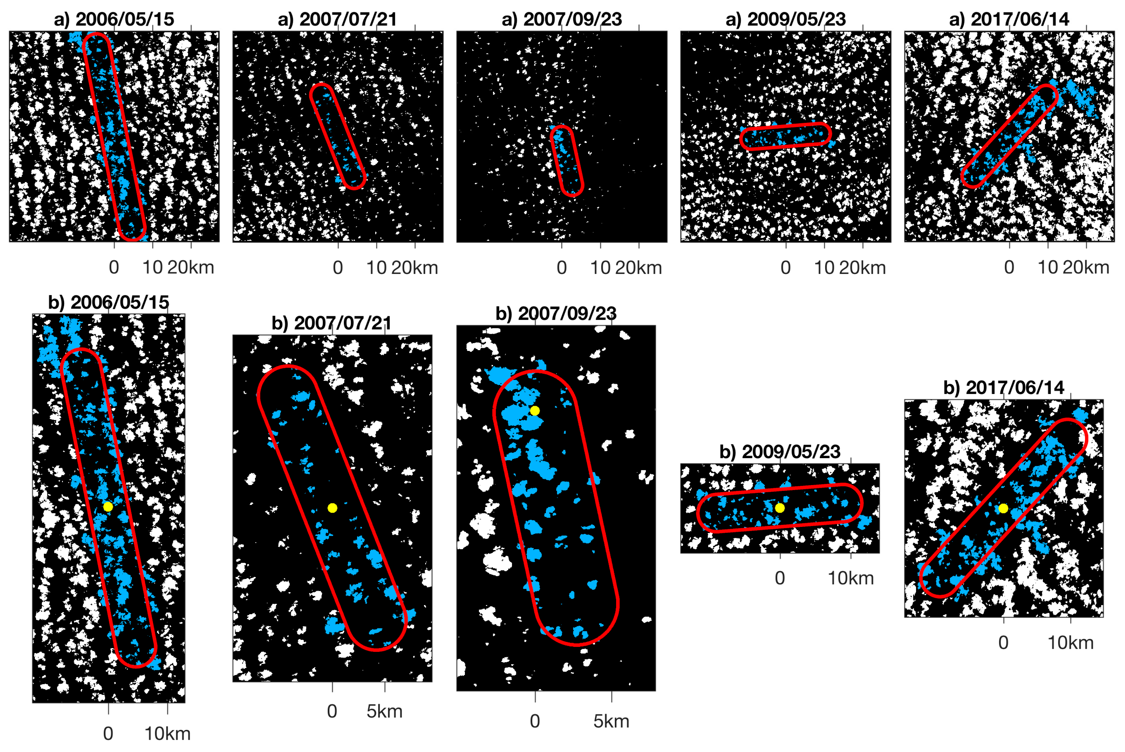
Landsat cloud mask for selected 5 days; Landsat cloud area obtained from the entirety of blue-tinted clouds, whereas simulated TSI-like cloud area (Section 4) is obtained from clouds strictly within the red outline subarea with variable dimensions (Table 1). (a) 50 km × 50 km region showing different spatial patterns of cloud cover and (b) zoomed in to red outline subarea observed by a theoretical TSI operating with a 130° FOV for 1 h on all days except 2007/09/23 for 30 min due to sun glare contamination. North is up and East is to the right. SGP site is indicated as yellow dot at the origin. The selected days represent a wide range of cloud fraction (0.04–0.33, see Table 1) and different spatial patterns of cloud cover.
Figure 4.
Landsat cloud mask for selected 5 days; Landsat cloud area obtained from the entirety of blue-tinted clouds, whereas simulated TSI-like cloud area (Section 4) is obtained from clouds strictly within the red outline subarea with variable dimensions (Table 1). (a) 50 km × 50 km region showing different spatial patterns of cloud cover and (b) zoomed in to red outline subarea observed by a theoretical TSI operating with a 130° FOV for 1 h on all days except 2007/09/23 for 30 min due to sun glare contamination. North is up and East is to the right. SGP site is indicated as yellow dot at the origin. The selected days represent a wide range of cloud fraction (0.04–0.33, see Table 1) and different spatial patterns of cloud cover.

Figure 5.
(a) 1-h averaged cloud fraction for TSI (red square), TSI-like sampling (green diamond) and within the Landsat subarea (navy circle). Error bars show the minimum and maximum 15-min average for TSI and TSI-like. (b) Percentiles of cloud cover density summarize population CED. Open symbols are the median (L50) for TSI (square, red), TSI-like (diamond, green) and Landsat (circle, navy) with 25th and 75th (box) and 5th and 95th (whiskers) percentiles.

Figure 6.
Distributions of CED from Landsat (navy), TSI (red) and TSI-like simulator (green) for 5 days. (a) subfigures of normalized cloud size distribution (Equation (2)). (b,c) cloud cover density (Equation (3)) compared for (b) TSI-like (turquoise) and Landsat (navy) and (c) TSI (red) and Landsat (navy). Note that Landsat cloud areas extend beyond the observed area S as shown in Figure 4.

Table 1.
Landsat cloud fraction (CF), cloud base height (CBH), wind speed and direction (dir.) at CBH, the estimated width and length of subareas (Figure 4b) for 130° FOV and 1-h averaging period. Numbers of clouds observed by TSI (N TSI) and Landsat (N Lsat).
Table 1.
Landsat cloud fraction (CF), cloud base height (CBH), wind speed and direction (dir.) at CBH, the estimated width and length of subareas (Figure 4b) for 130° FOV and 1-h averaging period. Numbers of clouds observed by TSI (N TSI) and Landsat (N Lsat).
| Landsat Scene | CF (50-km) | CF Subarea | CBH (km) | Wind Speed (m/s) | Wind dir. (deg) | Width (km) | Length (km) | N TSI | N Lsat |
|---|---|---|---|---|---|---|---|---|---|
| 2006/05/15 | 0.27 | 0.26 | 1.52 | 13.4 | 349 | 6.5 | 48.2 | 2445 | 297 |
| 2007/07/21 | 0.1 | 0.1 | 1.25 | 6.5 | 159 | 5.4 | 23.4 | 1483 | 87 |
| 2007/09/23 | 0.04 | 0.15 (1) | 1.25 | 7.2 | 168 | 5.4 | 25.9 | 1700 | 60 |
| 2009/05/23 | 0.17 | 0.16 | 1.24 | 5 | 85 | 5.3 | 18 | 2017 | 80 |
| 2017/06/14 | 0.33 | 0.3 | 1.3 | 7.8 | 223 | 5.6 | 28.1 | 4093 | 85 |
(1) Note that values of CF calculated for the 50-km (second column) and smaller subarea (third column) are comparable for all days considered here except 23 September 2007 where the subarea CF exceeds the 50-km CF more than three times likely due to the strong diurnal variability of CF before noon.
Table 2.
Comparison of median of the cloud cover density L50 and characteristic size λc for the cloud cover density, σ(λ), in Figure 6b,c.
Table 2.
Comparison of median of the cloud cover density L50 and characteristic size λc for the cloud cover density, σ(λ), in Figure 6b,c.
| Date | Statistic | Lsat (whole, km) (1) | Lsat (cut-off, km) (2) | TSI-Like (km) | TSI (km) |
|---|---|---|---|---|---|
| 2006/05/15 | L50 | 2.03 | 1.64 | 1.60 | 1.63 |
| λc | 2.48 | 1.75 | 1.73 | 1.69 | |
| 2007/07/21 | L50 | 1.11 | 0.79 | 0.93 | 0.93 |
| λc | 1.04 | 0.92 | 0.92 | 0.93 | |
| 2007/09/23 | L50 | 1.09 | 0.96 | 1.13 | 1.78 |
| λc | 1.35 | 1.32 | 1.27 | 1.79 | |
| 2009/05/23 | L50 | 1.39 | 0.96 | 1.17 | 1.15 |
| λc | 1.33 | 1.16 | 1.20 | 1.30 | |
| 2017/06/14 | L50 | 2.60 | 1.77 | 1.74 | 2.30 |
| λc | 2.79 | 2.30 | 2.05 | 2.06 |
(1) Whole refers to the primary analysis presented, where the clouds extending beyond the 130° FOV in the Landsat sub-area are kept whole (shaded clouds in Figure 4b). (2) Cut-off refers to the same clouds as in the primary analysis, except clouds extending beyond the 130° FOV boundary are truncated (red line in Figure 4b), the distribution of the cut-off clouds is not shown in Figure 6.
© 2018 by the authors. Licensee MDPI, Basel, Switzerland. This article is an open access article distributed under the terms and conditions of the Creative Commons Attribution (CC BY) license (http://creativecommons.org/licenses/by/4.0/).
Share and Cite
MDPI and ACS Style
Kleiss, J.M.; Riley, E.A.; Long, C.N.; Riihimaki, L.D.; Berg, L.K.; Morris, V.R.; Kassianov, E. Cloud Area Distributions of Shallow Cumuli: A New Method for Ground-Based Images. Atmosphere 2018, 9, 258. https://doi.org/10.3390/atmos9070258
AMA Style
Kleiss JM, Riley EA, Long CN, Riihimaki LD, Berg LK, Morris VR, Kassianov E. Cloud Area Distributions of Shallow Cumuli: A New Method for Ground-Based Images. Atmosphere. 2018; 9(7):258. https://doi.org/10.3390/atmos9070258
Chicago/Turabian StyleKleiss, Jessica M., Erin A. Riley, Charles N. Long, Laura D. Riihimaki, Larry K. Berg, Victor R. Morris, and Evgueni Kassianov. 2018. "Cloud Area Distributions of Shallow Cumuli: A New Method for Ground-Based Images" Atmosphere 9, no. 7: 258. https://doi.org/10.3390/atmos9070258
Note that from the first issue of 2016, this journal uses article numbers instead of page numbers. See further details here.