A Comparative Analysis of the Impacts of Two Types of El Niño on the Central and Eastern Pacific ITCZ

1
Institute of Meteorology and Oceanography, National University of Defense Technology, Nanjing 211101, China
2
Department of Military Oceanography, Dalian Naval Academy, Dalian 116018, China
*
Author to whom correspondence should be addressed.
Atmosphere 2018, 9(7), 266; https://doi.org/10.3390/atmos9070266
Submission received: 25 May 2018
/
Revised: 1 July 2018
/
Accepted: 13 July 2018
/
Published: 15 July 2018
(This article belongs to the Section Meteorology)
Abstract
:The precipitation data from the Global Precipitation Climatology Project (GPCP) and CPC Merged Analysis of Precipitation (CMAP) were used to investigate the discrepancy of Centre and Eastern Pacific ITCZ (CEP-ITCZ) during two types of El Niño years. Two models of the heat source distribution during two types of El Niño events were constructed, and the causes of different CEP-ITCZ anomalies for two types of El Niño events were analyzed through the Gill model. The results show that the CEP-ITCZ precipitation is approximately 4.0° southward, and the intensity is enhanced by 3.6 mm/day during the mature period of Eastern Pacific El Niño (EP-El Niño), while during the mature period of Central Pacific El Niño (CP-El Niño), it is only 0.8° southward, and the intensity is enhanced by 3.2 mm/day. The meridional mode of the SST anomaly by means of EOF (Empirical Orthogonal Function) can indirectly affect the CEP-ITCZ by influencing the atmospheric Rossby wave response. In CP-El Niño years, the meridional mode of the SST anomaly is weak, and the atmospheric Rossby wave response enhances the northern and southern trade-wind zones at the same time. The anomaly of cross-equatorial flow is weak and the CEP-ITCZ moves southward a little. At the same time, the wind convergence zone is enhanced, and it is more conducive to the vertical transport of water vapor. In EP-El Niño years, the meridional mode of the SST anomaly is strong, and the atmospheric Rossby wave response strengthens the meridional wind on the northern side of the equator, leading to the southward shift of the CEP-ITCZ. At the same time, the wind convergence zone is weakened and widened, and to a certain extent, it suppresses the vertical transport increase of water vapor caused by the sea surface evaporation.
1. Introduction
Intertropical Convergence Zone (ITCZ), as one of the important systems of the tropical atmosphere, has important impacts on global atmospheric circulation. Due to a range of factors, the regional ITCZ has different characteristics. Among them, the Central and Eastern Pacific ITCZ (CEP-ITCZ) is located to the north of the equator most of the time and shows high particularity relative to other regions. Xie et al. [1,2], Philander et al. [3], and Chang et al. [4] proposed positive feedback mechanisms for “wind-evaporating-SST”, “cloud-SST” and “the cross equatorial wind-upwelling current”, respectively, and also explained the reasons for the CEP-ITCZ continuously occurring to the north of the equator. Marshall et al. [5] and Frierson et al. [6] found that the mean position of the ITCZ north of the equator is a consequence of northwards heat transport across the equator by ocean circulation. Compared to the ITCZ in other regions, the season and interannual variation of CEP-ITCZ are small and are generally located at 5–8° N [7]. Sometimes, the double-ITCZ state may also occur during boreal spring, especially in March–April [8]. In addition to seasonal movement, the meridional position of CEP-ITCZ is usually affected by El Niño events. Vecchi et al. [9] and Lengaigen et al. [10] pointed out that in EP-EL Niño years, the Eastern Pacific ITCZ would be unusually southward. Sui et al. [11] found that the vertical velocity extremes of the Eastern Pacific ITCZ are southward in an El Niño year and northward in a La Niña year. Adam et al. [12] found that ITCZ variations driven by ENSO (El Niño-Southern Oscillation) are characterized by an equatorward (poleward) shift in the Pacific during El Niño (La Niña) episodes, which are associated with variations in equatorial ocean energy uptake. In addition, the impacts of two types of El Niño on the Eastern Pacific ITCZ are different. Xie et al. [13] found that the Eastern Pacific ITCZ is slightly southward in Central Pacific El Niño (CP-El Niño) year, and the southward extent is less than that in Eastern Pacific El Niño (EP-El Niño) year.
The latent heat resulting from water vapor condensation released by ITCZ, an important tropical system, has a direct driving effect on the atmosphere [14,15]. The CEP-ITCZ is geographically closest to the area where El Niño occurs and is directly forced by the SST (sea surface temperature) anomaly, which in turn changes the global atmospheric circulation. In an El Niño year, SST shows positive anomalies, sea surface evaporation increases, and the condensation latent heat released by ITCZ surges. A stronger heat source forcing effect occurs relative to ordinary years. At present, some theoretical models have been applied to explain the forcing of a tropical heat source on the tropical atmosphere. For example, by using linear equations, Webster [15] explained the atmospheric east wind anomalies excited by the eastern side of the equatorial symmetric heat source using the atmospheric equatorial Kelvin wave response. Gill [16] used barotropic primitive equations to explain the zonal asymmetric wind field anomaly and circulation anomalies on the northern and southern sides of the equator excited by the equatorial symmetric heat source using the equatorial Kelvin wave and the Rossby wave. Xing et al. [17] used the Gill model to obtain the analytic solution of the response of the tropical atmosphere to the single equatorial asymmetric heat source and to study the influence of the meridional position, width and intensity of the single heat source on the atmosphere. This Gill model is universal in studying atmospheric responses forced by the ocean and is successfully used to study and explain many anomalous circulation characteristics of the actual atmosphere [17,18,19,20].
Therefore, taking into account that the location and intensity of CP-El Niño and EP-El Niño are very different, their impacts on the CEP-ITCZ inevitably vary widely. Previous studies have not analyzed this variation in depth, especially the difference between the impacts of two types of El Niño on the intensity of CEP-ITCZ, and have not explained the reasons for this difference. Some scholars have pointed out that El Niño events after the 21st century are more inclined to be CP-El Niño [21,22,23,24,25,26]. The study of the differences in the impact of two types of El Niño on the CEP-ITCZ contributes to the future prediction of CEP-ITCZ anomalies through changes in El Niño events. Based on the analysis of precipitation data, the main differences between the CEP-ITCZ in two types of El Niño years are presented. A possible mechanism of two types of El Niño affecting CEP-ITCZ was proposed. The results presented in this paper are of great significance to the study of tropical sea-air interaction, climate prediction and numerical simulation assessment.
2. Information and Methods
2.1. Data
The monthly GPCP (Global Precipitation Climatology Project) and CMAP (CPC Merged Analysis of Precipitation) data from 1979 to 2015, with a resolution of 2.5° × 2.5° were used. GPCP was developed by the World Climate Research Program (WCRP). This program contains monthly average precipitation satellite-observation data integrated with microwave and infrared detection data, formed by the use of optimal mixed estimates [27,28,29]. CMAP contains monthly and annual global precipitation data. The standard version of the data incorporates rain gauge observations and satellite precipitation estimates [30,31]; based on this, the enhanced version of the data incorporates the NCEP reanalysis data, and the unit of monthly precipitation is mm/day. There is a gap between these data and the GPCP data, but the distribution of precipitation is roughly the same, with no contradiction.
The monthly mean data of the SST, wind field, geopotential height, and vertical velocity from 1979 to 2015 were obtained using ERA-Interim at a resolution of 1° × 1°. ERA-Interim is a global atmospheric reanalysis product developed by the European Center for Medium-Range Weather Forecasts (ECMWF). The start time was January 1979.
2.2. Selection of Two Types of El Niño Years
In order to select typical CP-El Niño and EP-El Niño years, the Central Pacific ENSO index (CPI) and Eastern Pacific ENSO index (EPI) proposed by Qin et al. [32] were used to describe two types of El Niño, which were calculated as follows:
SSTA is the regional average of the sea surface temperature anomaly in five sea areas, i.e., A, B, C, D, E. The five sea areas are:
are the defined weight coefficients according to the size of the sea area, with values as follows:
A (5° S–5° N, 110° W–80° W),
B (5° S–10° N, 150° E–180°),
C (10° S–10° N, 170° E–140° W),
D (10° S–5° N, 130° E–150° E),
E (5° S–5° N, 100° W–80° W).
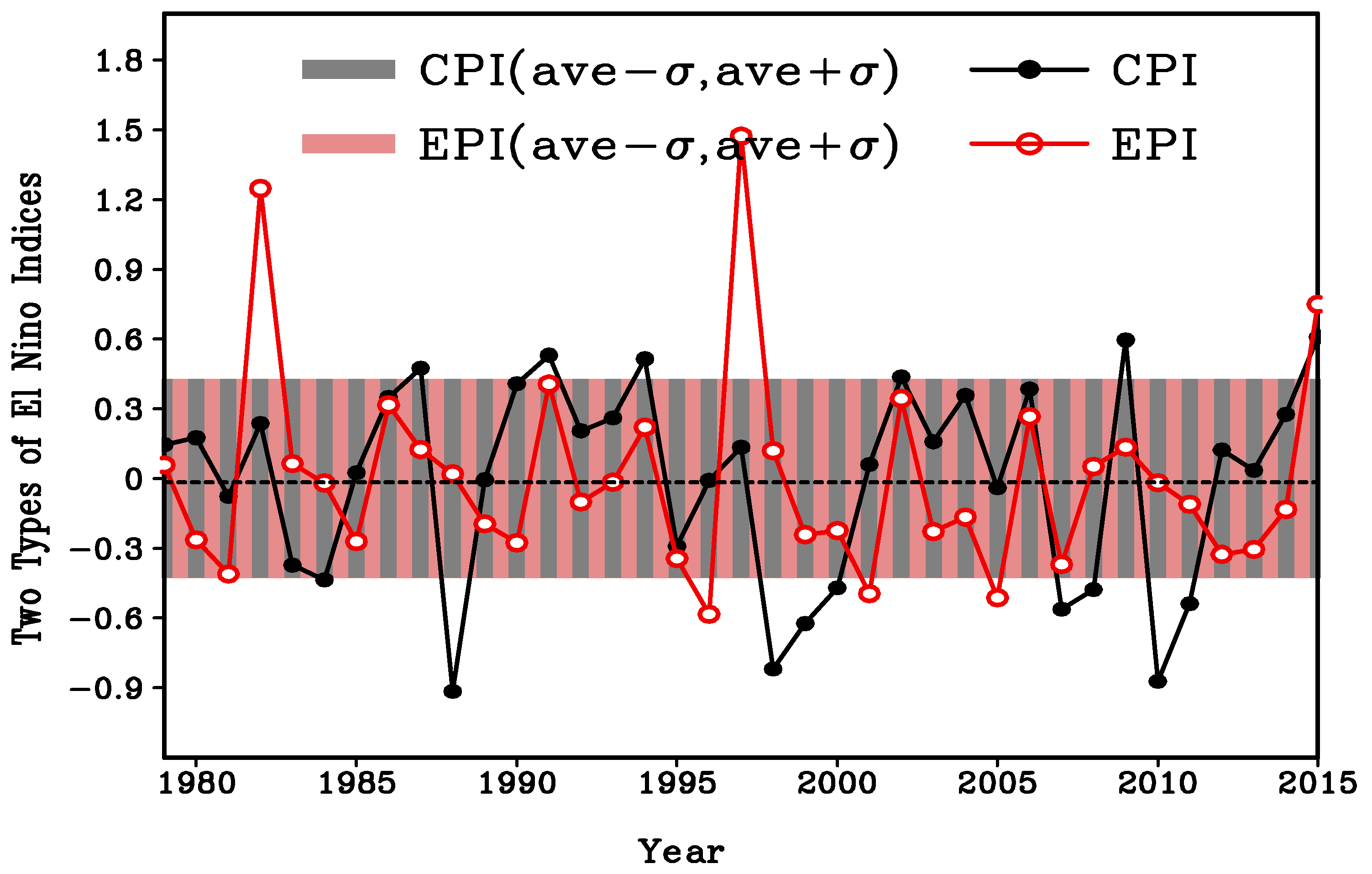
This classification method takes into account the sea surface temperature anomalies of each sea area in the low latitudes of the Pacific Ocean, not limited to the center and eastern Pacific, and this classification method is novel and computationally simple. The SST mean data from November to January of the following year from 1979 to 2015 were used, and two types of indices time series are shown in Figure 1. The shaded part of the figure is a standard deviation range for two types of indices, where the standard deviation of CPI is 0.427 and the standard deviation of EPI is 0.429. If the EPI of a year exceeds the EPI standard deviation and the CPI of the year does not exceed the CPI standard deviation, the year can be defined as a typical EP-El Niño year. It is not difficult to identify the typical EP-El Niño years in the figure, i.e., 1982/83 and 1997/98. Similarly, the typical CP-El Niño years (CP-El) include 1987/88, 1991/92, 1994/95, 2002/03, and 2009/10.
2.3. A Brief Description of the Gill Model
A heat source function could be expanded into a Weber function. By substituting the expanded item into the Gill model, the analytical solution of the atmospheric response can be obtained [17]. The heat source function and the solution process is in the Appendix.
In this paper, after expanding the heat source into the Weber function, only the first five items for solutions were used. The relative error of the heat source intensity is approximately 1.98% (Table 1).
3. The Different Characteristics of CEP-ITCZ Precipitation in Two Types of El Niño Years
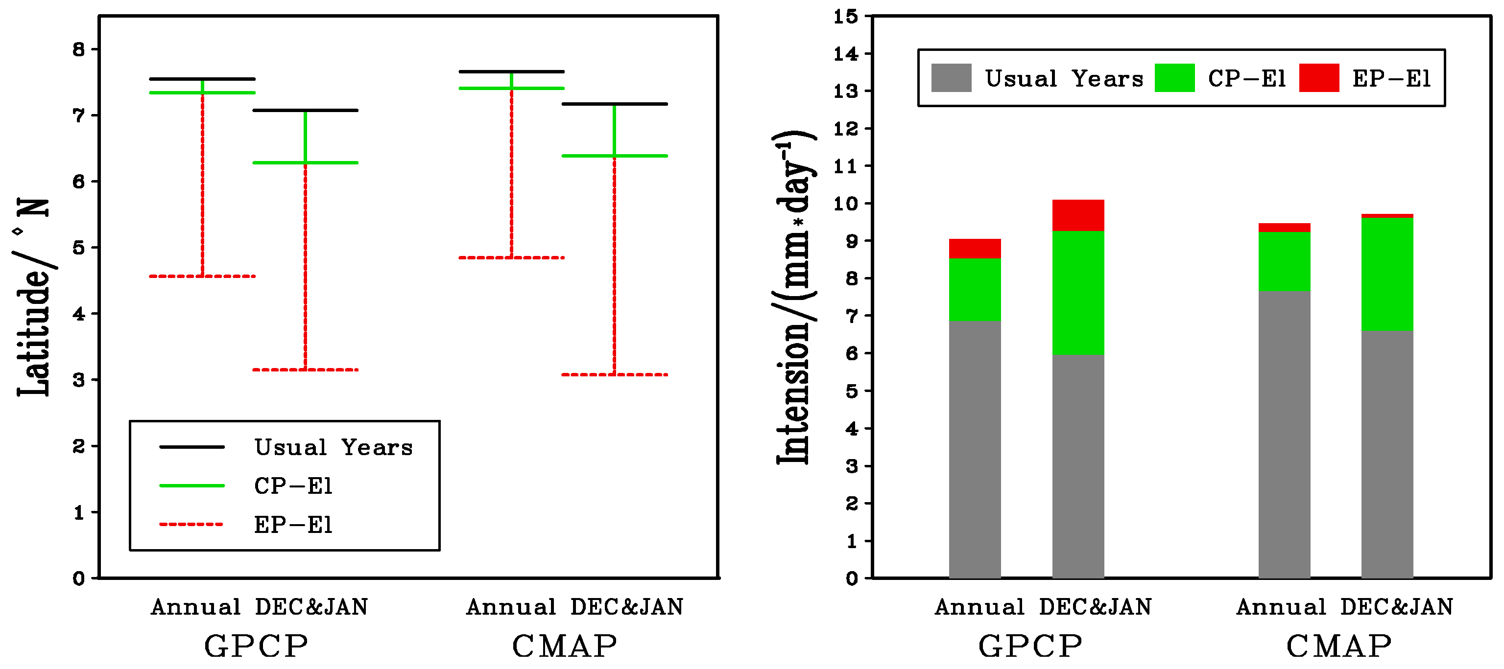
The definition of CEP-ITCZ defined by Ryan et al. [33] from the perspective of precipitation was used to analyze the anomalies of CEP-ITCZ position and intensity during two types of El Niño years in this paper. Figure 2 shows the annual mean offset of the CEP-ITCZ position and intensity in two types of El Niño years, and the offset during the mature period of El Niño. A comparison indicates that the effects of the two types of El Niño on CEP-ITCZ are very different, and the two types of precipitation data show the same result.
The GPCP (CMAP) data show that the annual mean CEP-ITCZ position in ordinary years is 7.6° N (7.7° N), and the mean position from December to the following January is 7.1° N (7.2° N). In EP-El Niño years, CEP-ITCZ’s annual mean position is southward 3.0° (2.8°), and southward 3.9° (4.1°) during the mature period of El Niño. In CP-El Niño years, CEP-ITCZ’s annual mean position is only 0.2° (0.2°) southward, and only 0.8° (0.8°) southward during the mature period of El Niño.
With respect to the CEP-ITCZ intensity, the GPCP (CMAP) data show that the annual mean is 6.9 mm/day (7.7 mm/day) in ordinary years, and 6.0 mm/day (6.6 mm/day) from December to the following January. In EP-EL Niño years, the annual mean intensity of CEP-ITCZ increases by 2.2 mm/day (1.8 mm/day) and by 4.1 mm/day (3.1 mm/day) during the mature period. In CP-EL Niño years, the annual mean intensity of CEP-ITCZ increases by 1.7 mm/day (1.6 mm/day) and by 3.3 mm/day (3.1 mm/day) during the mature period.
The EP-El Niño has a larger impact on the position and intensity of CEP-ITCZ, while the CP-El Niño has little effect on the position of CEP-ITCZ but almost the same impact on CEP-ITCZ intensity as the EP-El Niño. In general, the increased SST extent of the EP-El Niño is much larger than that of the CP-El Niño. The higher SST indicates stronger sea surface evaporation [34], and the CEP-ITCZ precipitation intensity should be much stronger as well. However, this is not consistent with the above statistical conclusions. What is the reason for the impact on the CEP-ITCZ intensity in the two types of El Niño years? The low-level atmospheric flow fields were analyzed first.
4. Comparative Analysis of Atmospheric Flow Fields
Wind Field
ITCZ is the result of the convergence of the Northern and Southern Hemisphere trade winds in the lower tropics. The meridional position is largely determined by the relative strength of the Northern and Southern Hemisphere trade winds. Under normal circumstances, in the Central and Eastern Pacific, the southeast trade wind is stronger than the northeast trade wind. The northward cross-equator flow occurs throughout the year. Therefore, CEP-ITCZ is located in the Northern Hemisphere year round.
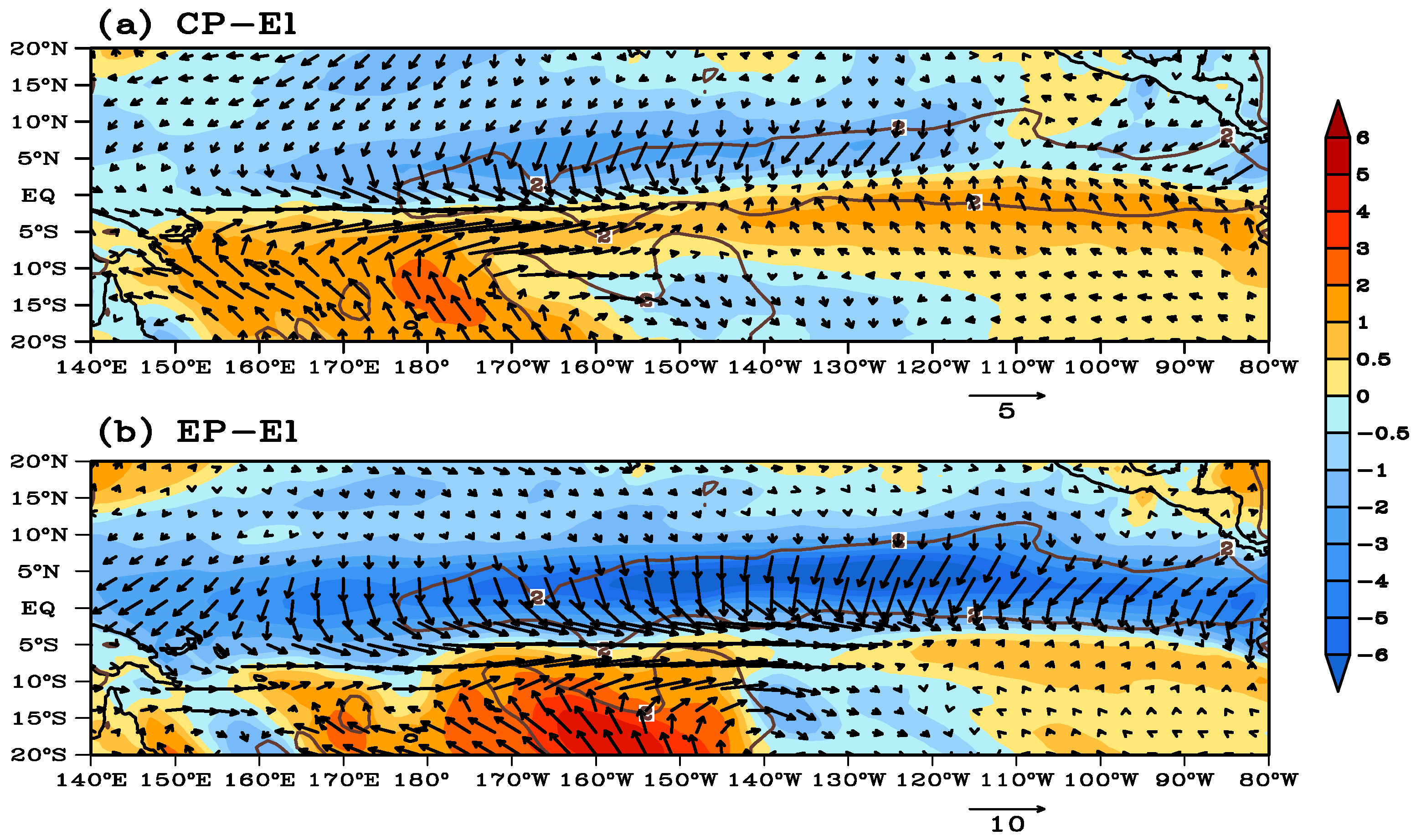
Figure 3 shows wind field anomalies of the low-level atmosphere during the mature period of two types of El Niño. The area within the grey contour line passed the 95% significance test, indicating that there is a significant difference in wind fields between two types of El Niño years. In CP-EL Niño, the anomalous wind fields in the Central and Eastern Pacific are symmetrically distributed along the equator. The northerly wind is in the Northern Hemisphere, and the southerly wind is in the Southern Hemisphere, and there is no significant difference in the wind speed. This means that in CP-EL Niño years, the trade wind in both the Northern and Southern Hemispheres increases over the Central and Eastern Pacific, leading to strengthened wind convergence and no large offset of the ITCZ location. In EP-EL Niño years, the anomalous wind field over the Central and Eastern Pacific is relatively strong. A stronger northward wind appears in the Northern Hemisphere, whereas the wind field anomaly in the Southern Hemisphere is very small, leading to the emergence of the cross-equator flow from north to south. This cross-equator flow enhances the Northern Hemisphere trade wind and weakens the Southern Hemisphere trade wind, resulting in a larger southward movement of the CEP-ITCZ in EP-EL Niño years.
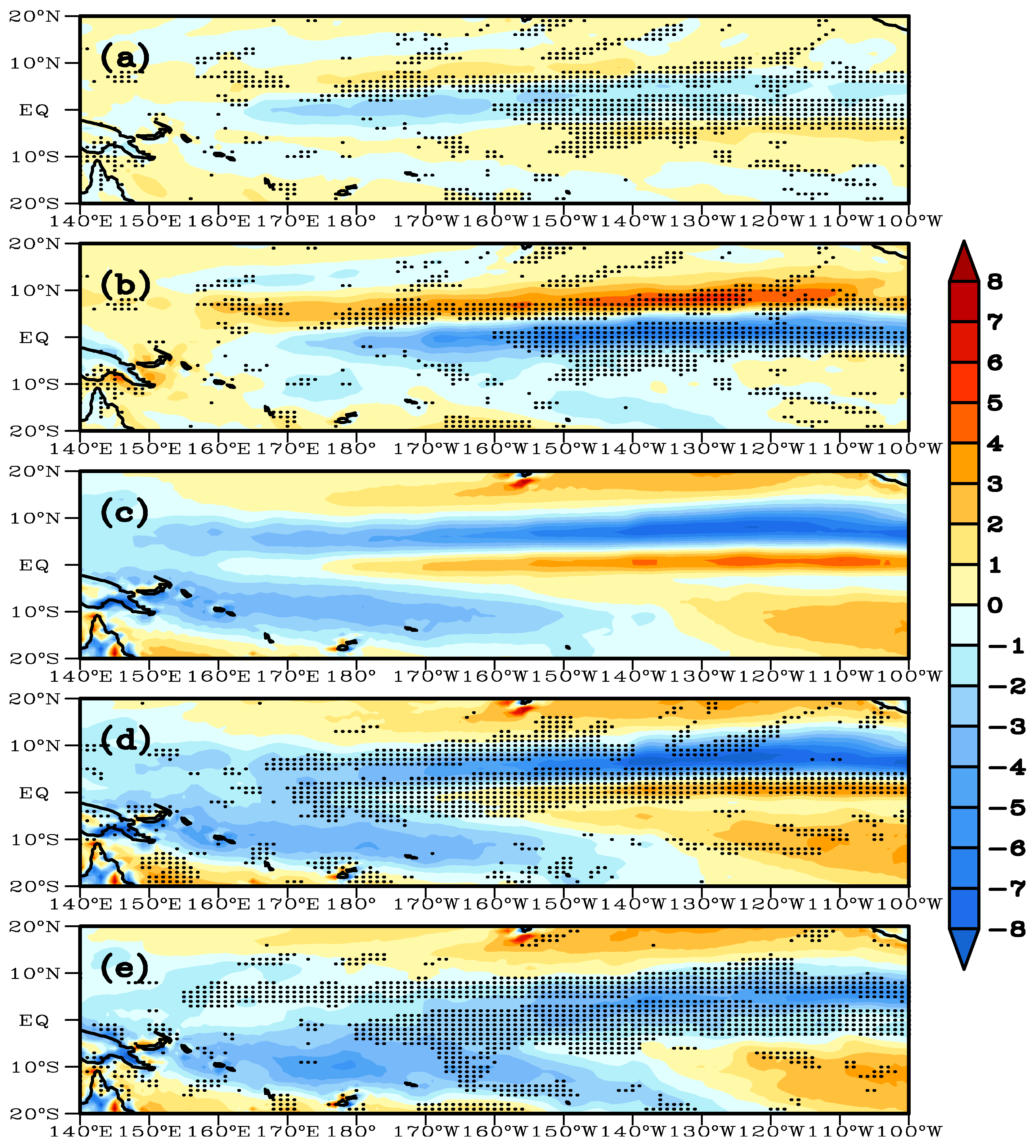
Figure 4 shows the divergence anomaly and divergence field of the low-level atmosphere during the mature period of two types of El Niño. The dots passed the 95% significance test, where (a) and (b) show significant differences between two types of El Niño years, (d)/(e) and (c) show significant differences between CP-El /EP-El Niño years and ordinary years. During the mature period of CP-El Niño, the tropical Pacific shows a negative divergence anomaly (Figure 4a), extending up to ± 5° in the Northern and Southern Hemisphere with a central intensity of approximately −2 × 10⁻⁵ s−1, while the positive divergence anomaly is relatively weak. During the mature period of EP-El Niño years, the divergence anomaly in the Central and Eastern Pacific presents a dipole structure (Figure 4b). The negative anomaly is located near the equator, and the central intensity reaches −6 × 10⁻⁵ s−1. The positive anomaly occurs on the northern side of the negative anomaly, at approximately 5–10° N, with a central intensity reaching 5 × 10⁻⁵ s−1. This dipole structure is formed by its strong anomaly of meridional wind.
The different structures of the divergence anomalies during two types of El Niño years results in divergence fields with different characteristics. Compared to the divergence field of the low-level atmosphere in ordinary years (Figure 4c), the divergence field structure in CP-EL Niño years does not change much (Figure 4d), but there is a stronger convergence and the central intensity increases from −6 × 10⁻⁵ s−1 to −8 × 10⁻⁵ s−1 However, the divergence field in EP-EL Niño years is obviously widened (Figure 4e). The southern boundary of the convergence zone extends from near the equator to near 5° S, about one-third of the widening. The central intensity is reduced from −6 × 10⁻⁵ s−1 to −4 × 10⁻⁵ s−1.
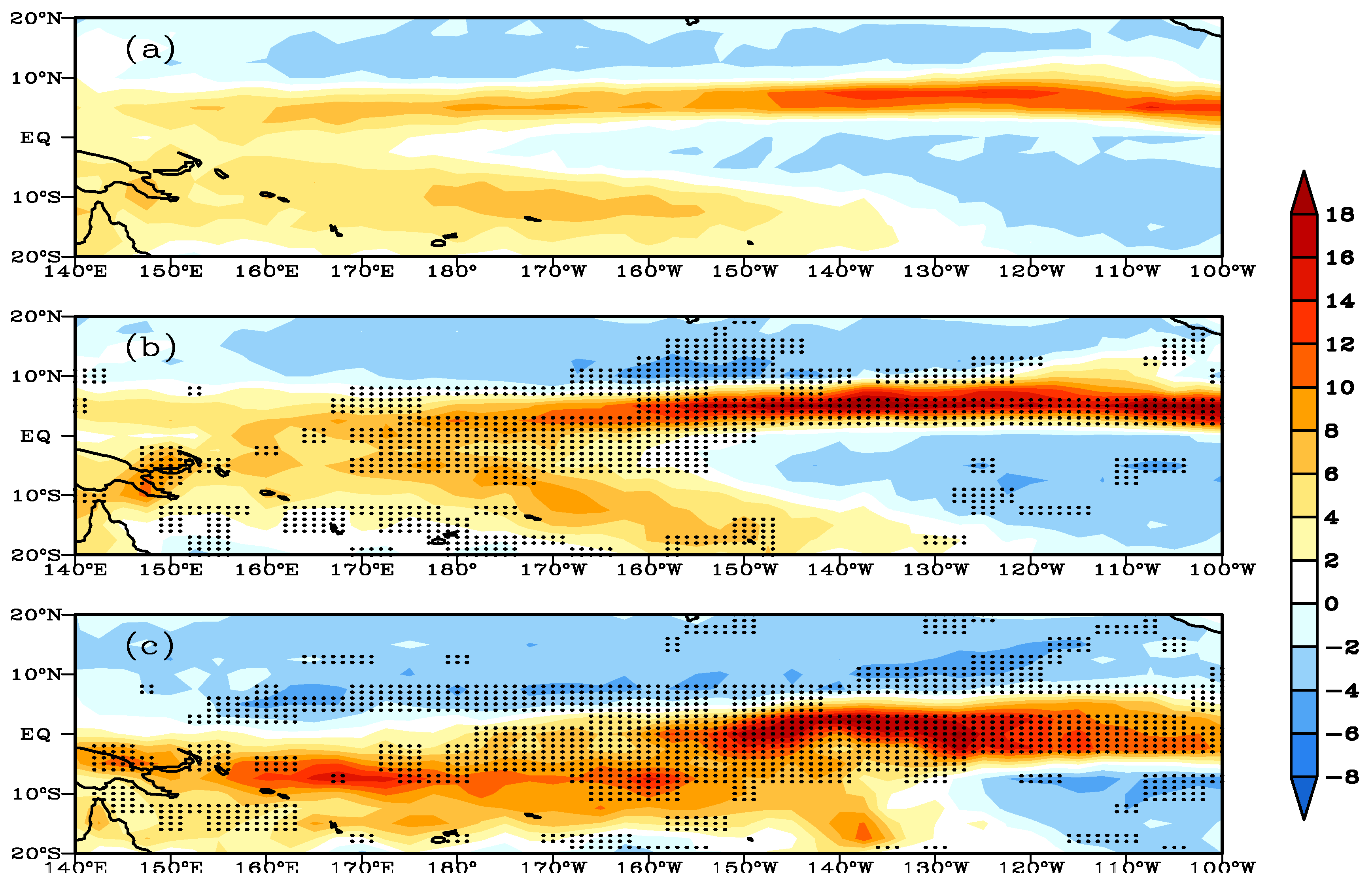
Therefore, although the intensity of the SST anomaly of CP-El Niño is much weaker than that of EP-El Niño, the abnormal atmospheric circulation excited by it is more favorable to the convergence of ITCZ, thus creating more favorable conditions for the vertical transport of water vapor. However, for EP-El Nino, although there is a stronger SST anomaly which is conducive to increasing the sea surface evaporation, the excited atmospheric circulation anomaly increases the width and weakens the central intensity of the convergence zone. To some extent, this inhibits the speed of the vertical transport of water vapor. As shown in Figure 5, the maximum vertical water vapor flux at 850 hPa (Figure 5a) in ordinary years is 12 (unit: 10−5 g m−2 s−1, the same below). The increase in the vertical water vapor flux in CP-EL Niño years (Figure 5b) is the same as that in EP-EL Niño years (Figure 5c), with a maximum exceeding 15, and in some local areas, the increase in CP-EL Niño years exceeds that in EP-EL Niño years, up to 18 or more. Therefore, even if the increase of SST in CP-EL Niño years is much weaker than that in EP-EL Niño years, its impacts on the intensity anomalies of CEP-ITCZ are comparable to those in EP-EL Niño years.
5. Effects of SST on CEP-ITCZ
The above anomalous atmospheric wind field must be caused by the anomalous SST of two types of El Niño. Through the analysis of MV-EOF (Multivariate Empirical-Orthogonal-Function) of SST-precipitation, it is found that the SST anomaly of two types of El Niño has important effects on CEP-ITCZ precipitation. The results of MV-EOF is shown in Figure 6. The North [35] test is used to determine whether the mode is meaningless noise by calculating the eigenvalue error range of each mode. The method of calculation is
where is the eigenvalue of the jth mode, n is the number of independent samples, and the term on the right hand of the inequality is the error range of the eigenvalue . If the above inequality holds, it means that the corresponding empirical orthogonal function is a meaningful signal. The eigenvalues of the first two modes obtained from MV-EOF are shown in Table 2, and the results were verified using the North test.
The variance contribution of the first mode of the SST anomaly is 28.2%. The center of the positive anomaly is located in the equatorial region of the Central and Eastern Pacific. The corresponding first mode of precipitation shows that when the first mode of SST exhibits a positive anomaly, the precipitation in the equatorial region of the Central and Eastern Pacific is significantly increased, and the increase in the Central Pacific is stronger than that in the Eastern Pacific. The time coefficients of the first mode in two types of El Niño years are positive anomalies, and the one in EP-EL Niño years (the year marked “◀”) is stronger than that in CP-EL Niño years (the year marked “▶”). That is, the first mode of the SST anomaly increases CEP-ITCZ precipitation in two types of El Niño years, with only a difference in intensity.
The variance contribution of the second mode of the SST anomaly is 11.9%. The positive anomaly center of the spatial distribution is located in the equatorial region 170° W and extends to a northeasterly direction in the shape of a narrow and long belt. The negative anomaly center is located in the slightly southward equatorial area along the East Pacific coast. The corresponding positive and negative anomaly centers of the second mode of precipitation have a zonal distribution across the Pacific. However, when only the Central and Eastern Pacific is observed, it is found that the negative anomaly center is located in the equatorial region, and there is a weak positive anomaly on its northern side, i.e., the positive and negative anomalies in the Central and Eastern Pacific have meridional distribution. The time coefficients of the second mode have opposite signs to each other in two types of El Niño years. In EP-EL Niño years, the time coefficient is a very strong negative anomaly, compared with a weak positive anomaly in CP-EL Niño years. This suggests that in EP-EL Niño years, precipitation in the Central and Eastern Pacific will increase in the equatorial region and decrease in the north of the equator, resulting in a southward movement of CEP-ITCZ precipitation.
In summary, the effect of the first mode of the SST anomaly on the CEP-ITCZ precipitation in two types of El Niño years is only reflected by the difference in intensity of precipitation. The influence of the second mode of the SST anomaly may be the main cause of the difference in the position of CEP-ITCZ precipitation in the two types of El Niño years.
6. The Atmospheric Response Model of Two Types of El Niño
SST increases and the latent heat released by the sea surface evaporation is considered as a heat source of the atmospheric forcing. In order to further study the mechanism of the impact of the second mode of the SST anomaly on CEP-ITCZ, the Gill model was used to construct atmospheric response models of two types of El Niño events. Based on the model, the impact of two types of El Niño on CEP-ITCZ is discussed in greater depth.
6.1. The Design of the Atmospheric Heat Source
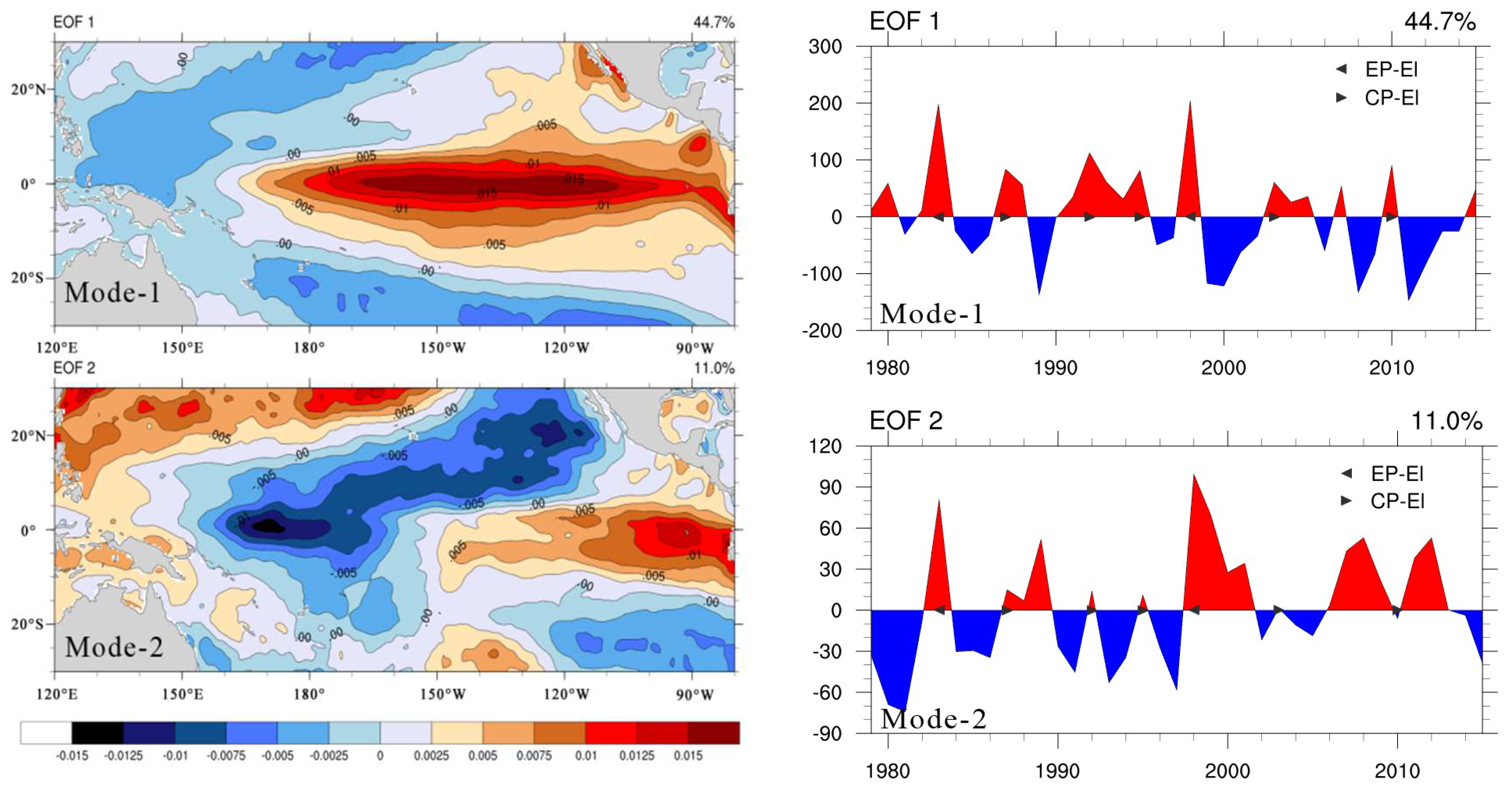
The first two modes can be obtained by EOF of the SST anomalies in the low-latitude Pacific. The results are shown in Figure 7. The eigenvalues of the first two modes are shown in Table 3, and the results were verified using the North test.
The variance contribution of the first mode is 44.7%. Its formation is mainly related to the El Niño event, which can be called the Niño mode [36]. Its spatial distribution is a positive anomaly in the equatorial region. The center is located along the equator and is a zonal distribution. The intensity decreases gradually from the equator to the north and south. The gradient on the northern side is slightly larger than that on the southern side. The meridional range of the positive anomaly is approximately 15° S–10° N, and the zonal range is approximately 160° E–80° W. As can be seen from the time coefficient, the Niño mode is positive for both types of El Niño years (the year marked “◀” is EP-El Niño, and the year marked “▶” is CP-El Niño). In order to simulate that the Niño mode positive anomaly center is located on the equator and the gradient in the Northern Hemisphere is slightly larger than that in the Southern Hemisphere, two heat sources with different intensity are superimposed to obtain the meridional asymmetric heat source centered on the equator. The intensities and meridional positions of the two heat sources satisfy the following conditions:
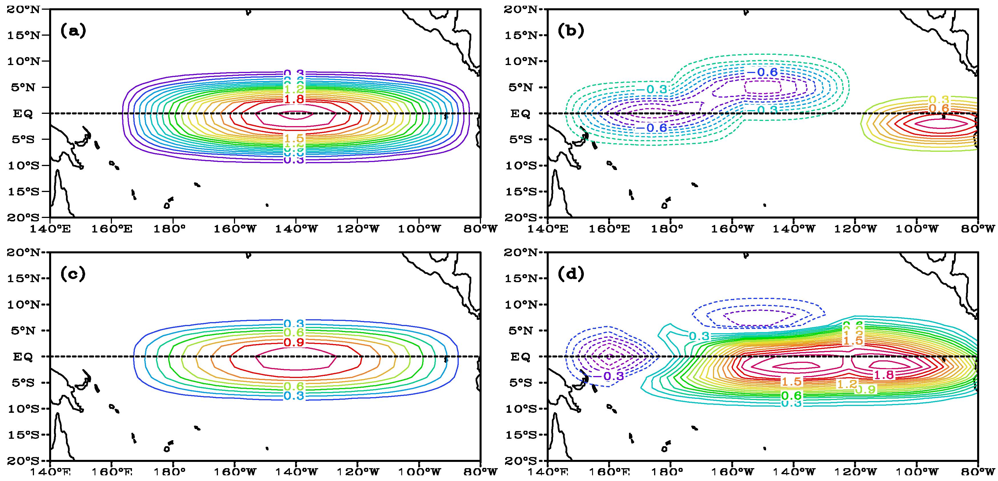
where are the intensities of the two heat sources; are the distances from the center of the two heat sources to the equator, and the positive (negative) value is located in the Southern (Northern) Hemisphere. The intensities of the two heat sources in CP-El Niño are set to half of that in EP-El Niño. The specific parameters are shown in Table 4, and the spatial distribution of the heat source is shown in Figure 8a.
The variance contribution of the second mode is 11.0%. This is the dominant mode of the SST anomalies after subtracting the Niño mode information. Some scholars call this the meridional mode [37,38], and they believe its formation is mainly related to the positive feedback mechanism of “Wind-evaporative-SST”. In its spatial distribution field, there is a positive anomaly along the coast of the Americas, with a central location on the southern side of the equator. The negative anomaly area is observed as a long and narrow belt in the northeast-southwest direction, and the center of the negative anomaly is located in the equatorial region 170° E. The heat source distribution of the meridional mode can be simplified as the superposition of two cold sources and one heat source, in which the equatorial region of the western Pacific is the first cold source, the equatorial northern side of the central Pacific is the second cold source, and equatorial southern side of the eastern Pacific coast is the heat source. From the time coefficient, it can be seen that the meridional mode develops strongly in EP-EL Niño years, while in CP-EL Niño years, it is significantly weakened. Therefore, the intensity of the heat source in EP-EL Niño is taken as 1, the intensity of the cold source is taken as −1, and in CP-EL Niño, all values are taken as 0. The spatial distribution of the heat source is shown in Figure 8b.
The design of the above-mentioned heat source not only considers the ratio of the strength between two modes but also the intensity relationship among the heat sources. The final heat source distribution models of two types of El Niño are shown in Figure 8c,d.
6.2. Results of the Atmospheric Response
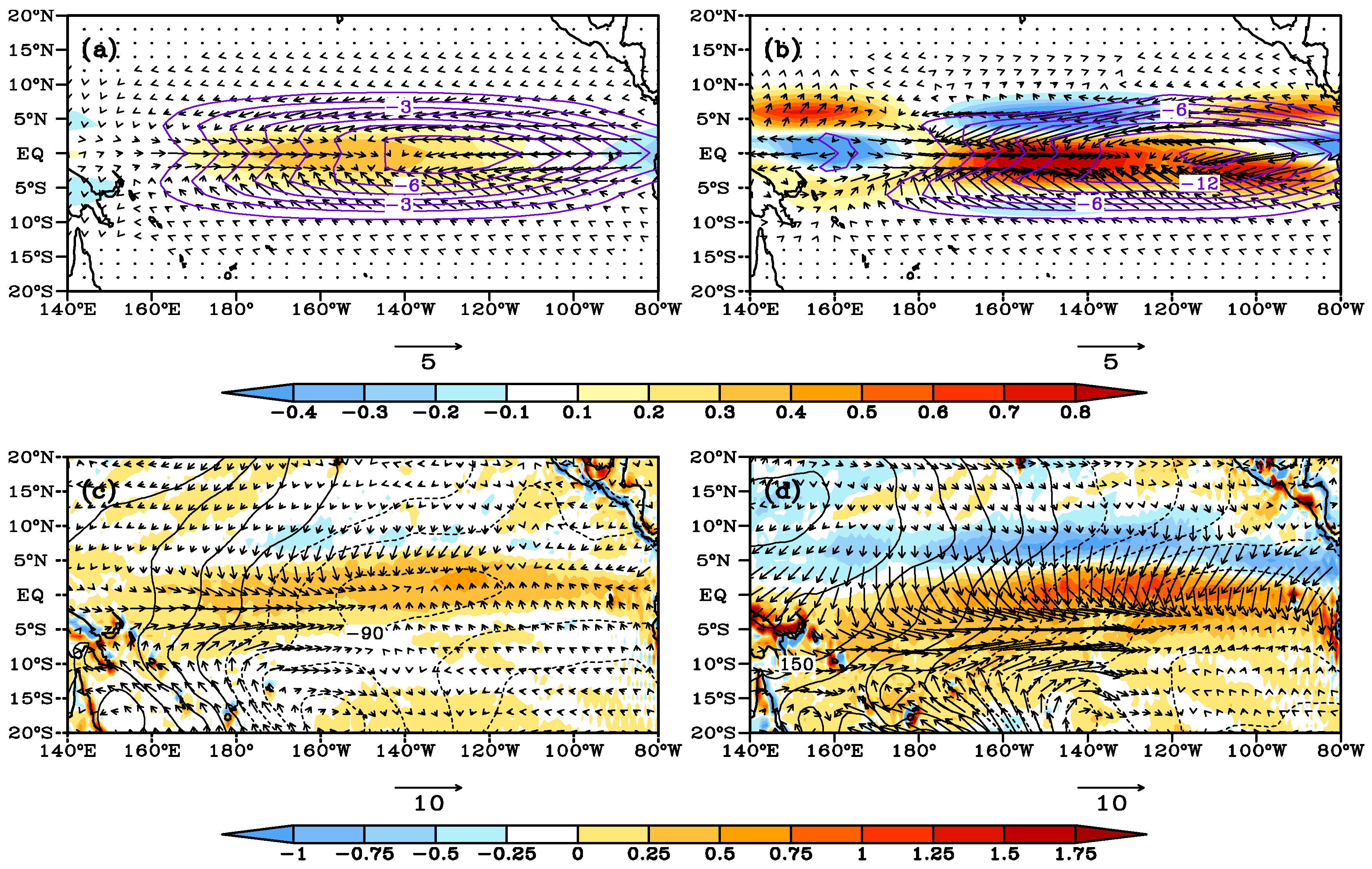
The atmospheric anomalies excited by the heat sources of two types of El Niño are shown in Figure 9a,b. The actual atmospheric anomalies during two types of El Niño years are shown in Figure 9c,d. It can be seen that the Gill model simulates some interesting atmospheric characteristics in the equatorial Pacific region during two types of El Niño years.
During CP-El Niño, the maximum value of the vertical velocity appears over the equator and gradually weakens towards the northern and southern sides. There is a strong westerly wind anomaly in the 160° E–160° W area of the equator and its southern side, and the flow field on both sides is cyclonic. A convergence wind field symmetrical to the equator appears in the central Pacific. The eastern Pacific is dominated by easterly winds. The low-pressure centers of the model and the actual atmosphere appear in the 140° W–120° W area of the equatorial region. Due to the Rossby wave of the low latitude, near 5° S and 5° N, there are pressure troughs extending westward from the low-pressure center to the west, and the trough in the Southern Hemisphere is stronger than that in the Northern Hemisphere.
During EP-El Niño, the positive anomaly of the vertical velocity also appears near the equator, with stronger intensity, and its meridional position in the east of 110° W becomes southward. The negative anomaly appears near 5° N, i.e., the airflow rises near the equator and sinks at 5° N. The westerly wind anomalies appear in the 180° W–140° W region on the southern side of the equator. There are northerly winds and the cross-equator flow from north to south on the northern side of the equator in the central and eastern Pacific. The low-pressure center on the equator appears at 120° W–100° W in the model and in the actual atmosphere. The pressure troughs in the Northern and Southern Hemispheres exhibit obvious meridional asymmetry. The pressure trough in the Southern Hemisphere is significantly stronger than that in the Northern Hemisphere.
Of course, there is a lot that is not captured by the Gill mode. For example, during CP-El Niño, maybe affected by the American mountains, the easterly winds over the eastern Pacific are weak in the actual atmosphere. During EP-El Niño, in the actual atmosphere, there are stronger northerly winds and the cross-equator flow from north to south. The northerly winds and the cross-equator flow in the model are weaker. And the southward degree of the westerly wind anomalies in the model is weaker than that in the actual atmosphere.
Although there is a lot that is not captured by the Gill mode, these differences are not concerned in this paper. In summary, the model shows some interesting characteristics of the atmospheric anomalies in the 10° S–10° N region of the Pacific during two types of El Niño years. The heat sources of the CP-El Niño does not have the superposition of the meridional mode of SST anomalies, and the atmospheric anomalies have better meridional symmetry, while the atmospheric anomalies during EP-El Niño are relatively complex.
6.3. Equatorial Kelvin Wave and Rossby Wave
The analytic solutions of the equatorial Kelvin wave and the Rossby wave in the model can be drawn separately. The horizontal structures of the two kinds of waves are shown in Figure 10a,b. It can be seen that the wind fields of the Kelvin waves are easterly winds, and the low-pressure central position on the equator is basically consistent with the actual atmosphere. The atmospheric anomalies are symmetrical along the equator, and the positive and negative values of the vertical velocity anomalies exhibit zonal distribution, while the anomalies of the CEP-ITCZ are mainly meridional changes. Therefore, it can be deduced that the wind-pressure structure of the Kelvin wave has no significant impact on the meridional position of the CEP-ITCZ.
There is meridional asymmetry in the structure of the Rossby wave (Figure 10c,d). In the model of CP-El Niño, the anomalies of the westerly winds are basically located near the equator, and the ascending motion occurs in the equatorial region. The structure of the Rossby wave is quasi-symmetrical along the equator. In the model of EP-El Niño, the anomalies of the westerly winds are located on the southern side of the equator, there is a strong ascending motion in the equatorial region of the central and eastern Pacific, and there is a strong downward motion on the northern side. The meridional distribution of the anomalies of the vertical velocity may have an effect on the north-south movement of the CEP-ITCZ. It can be inferred that the atmospheric Rossby wave excited by the SST anomalies may have a significant effect on the CEP-ITCZ.
Figure 11 shows the meridional wind speed and the divergence field of the above-mentioned Rossby wave. In the model of CP-El Niño, the meridional winds on both sides of the equator are distributed symmetrically along the equator in opposite directions with a similar wind force. The convergence zone is also distributed along the equator in the shape of a belt. This is consistent with the meridional winds in Figure 3a and the convergence zone in Figure 4a. In the model of EP-El Niño, the northern side of the equator has strong northerly winds, and the maximum wind speed can reach twice as high as that of the southerly winds on the southern side of the equator. The cross-equatorial flow from north to south appears on the equator. The convergence zone is on the equator, and there is a strong divergence zone near 5° N, which is also consistent with the results presented in Figure 3b and Figure 4b. Therefore, the atmospheric Rossby wave excited by the ocean may play an important role in the CEP-ITCZ anomalies in two types of El Niño years.
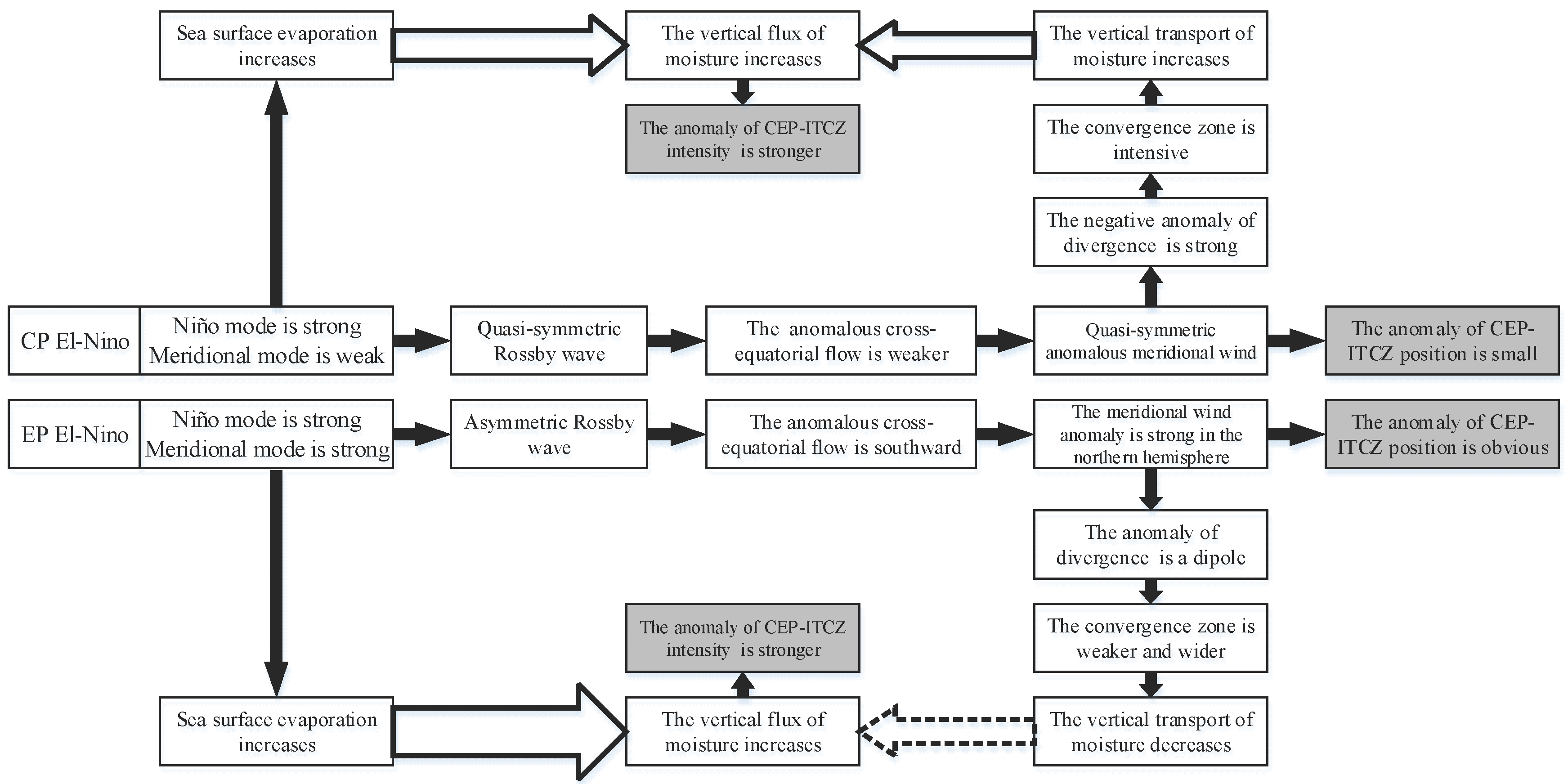
In summary, the heat source distributions established in this paper well simulated the atmospheric response to two types of El Niño events in the Gill model. The low-latitude atmospheric Rossby wave excited by SST anomalies can affect the CEP-ITCZ position by adjusting the cross-equatorial flow, enhance the convergence zone in CP-EL Niño years and widen and weaken the convergence zone in EP-EL Niño years. The meridional mode of the SST anomaly is also an important reason for the difference of the atmospheric Rossby wave response in two types of El Niño. Its mechanism is summarized in Figure 12.
7. Discussion and Conclusions
There is a complex sea-air interaction between El Niño and ITCZ. In this paper, the position and intensity anomalies of the CEP-ITCZ in two types of El Niño years were quantified by precipitation data and the direct cause of the changes of the CEP-ITCZ in two types of El Niño years was conducted. By establishing an atmospheric heat source model of two types of El Niño, it was found that the meridional mode of the SST anomaly plays an important role in the anomalies of the CEP-ITCZ by influencing the atmospheric Rossby wave response. The main conclusions are as follows.
(1) During CP-El Niño years, the anomalies of the meridional winds in the Northern and Southern Hemispheres are comparable, resulting in little changes in the CEP-ITCZ position. During EP-El Niño years, the anomaly of the meridional wind in the Northern Hemisphere is stronger, resulting in a higher extent of southward movement for the CEP-ITCZ.
(2) Compared with CP-El Niño, although the stronger sea surface evaporation during EP-El Niño is more conducive to enhancing CEP-ITCZ precipitation, the flow field in EP-El Niño years increases the width and weakens the central intensity of the convergence zone and inhibits the speed of the vertical transport of water vapor to a certain extent, while the flow field in CP-El Niño years enhances the convergence zone, which is more favorable for the vertical transport of water vapor. Thus, the precipitation intensities of the CEP-ITCZ in two types of El Niño years are similar.
(3) The meridional mode of the SST anomaly may be the root cause of the difference in the CEP-ITCZ between two types of El Niño years. It can result in the above-mentioned anomalous wind field and the divergence field by influencing the atmospheric Rossby wave response.
If El Niño events are more inclined to be of CP-El Niño after the 21st Century, the position anomaly of the CEP-ITCZ in El Niño years may be small, and the intensity anomaly will remain very strong. Although the atmospheric response excited by the model of the heat source designed in this paper explains the atmospheric anomalies in two types of El Niño years to a certain extent and provides a preliminary explanation for the differences of the CEP-ITCZ anomalies in two types of El Niño years, the Gill model has limitations. For example, the Gill model does not apply to a heat source located far from the equator and does not consider the influence of the atmospheric basic flow and mid-latitude system or the role of the Central American terrain. The key problem is that the method used in the paper does not account for the strongly coupled nature of the problem. In the context of climate warming, the interaction between the quietly changing El Niño event and ITCZ is extremely complex. Adam [39] proposed a simple shallow water model with an idealized Bjerknes feedback and studied the equatorially symmetric features of the bifurcated ITCZ pattern successfully. This idealized Bjerknes feedback could provide a conceptual framework for studying the large-scale features of ITCZ and the tropical circulation. Whether this conceptual framework can be used to further reveal the impact of two types of El Nino on CEP-ITCZ is unknown.; further research is needed.
Author Contributions
Methodology, J.Z.; Software, J.Z. and R.X.; Validation, J.Z., Y.L. and R.X.; Formal Analysis, J.Z.; Resources, H.C.; Data Curation, H.C. and J.Z.; Writing-Original Draft Preparation, J.Z.; Writing-Review & Editing, J.Z, Y.L., R.X. and H.C.; Visualization, J.Z. and R.X.; Supervision, Y.L.; Project Administration, Y.L. and J.Z.; Funding Acquisition, Y.L. All the authors have read and approved the final manuscript.
Funding
This research was funded by the National Natural Science Foundation of China (41175089).
Acknowledgments
The authors gratefully acknowledge the data supports by the ECMWF (European Centre for Medium Range Weather Forecasts) and NOAA (National Oceanic and Atmospheric Administration).
Conflicts of Interest
The authors declare no conflict of interest.
Appendix A
The following equation is obtained by nondimensionalizing the barotropic primitive equations, taking into account the steady solution and introducing the dissipation coefficient [16,40]:
where ε is the dissipation coefficient, and its value in this paper is 0.1; u and v are zonal and meridional winds, respectively; p is the pressure; w is the vertical velocity and Q is the heat source. The single heat source function used in this paper is as follows [17]:
where A is the heat source intensity; d is the distance from the center of the heat source to the equator; the positive (negative) value represents the center of the heat source in the Southern (Northern) Hemisphere, and L is the zonal distance of the heat source center decreasing to 0.
Set . Variables q, r, and v are expanded with elliptic cylindrical functions, and the following equation is obtained [16]:
The heat source function Q is expanded into a Weber function. By substituting the expanded item into each of the above equations, the analytical solution of the corresponding equation can be obtained.
Substituting the first item of the expanded heat source function Q (i.e., n = 0)
into Equations (5)–(7), two solutions are obtained. The first solution represents the eastward Kelvin wave, in the form of
where is the following piecewise function:
The second solution represents the westward Rossby wave, in the form of
where is the following piecewise function:
Substituting the second item of the expanded heat source function Q (i.e., n = 1)
into Equations (5)–(7), two solutions are obtained. The first solution represents the mixed Rossby-gravity wave, in the form of
The second solution is the Rossby wave, in the form of
where is the following piecewise function
The higher order terms of the expanded heat source function Q (i.e., n > 1) are expressed in the general formula:
After substituting the formula of higher order terms into equations, only one solution is obtained, in the form of
where is the following piecewise function
References
- Xie, S.P.; Philander, S.G.H. A coupled ocean-atmosphere model of relevance to the ITCZ in the eastern Pacific. Tellus 1994, 46, 340–350. [Google Scholar] [CrossRef]
- Xie, S.P. Westward propagation of latitudinal asymmetry in a coupled ocean-atmosphere model. J. Atmos. Sci. 1996, 53, 3236–3250. [Google Scholar] [CrossRef]
- Philander, S.G.; Gu, D.; Halpern, D.; Li, T.; Halpern, D.; Lau, N.-C.; Pacanowski, R.C. Why the ITCZ is mostly north of the equator. J. Clim. 1996, 9, 2958–2972. [Google Scholar] [CrossRef]
- Chang, P.; Ji, L.; Li, H.; Penland, C.; Matrosova, L. Predicting decadal sea surface temperature variability in the tropical Atlantic Ocean. Geophys. Res. Lett. 1998, 25, 1193–1196. [Google Scholar] [CrossRef]
- Marshall, J.; Donohoe, A.; Ferreira, D.; McGee, D. The ocean’s role in setting the mean position of the Inter-Tropical Convergence Zone. Clim. Dyn. 2013, 42, 1967–1979. [Google Scholar] [CrossRef] [Green Version]
- Frierson, D.M.W.; Hwang, Y.T.; Fučkar, N.S.; Seager, R.; Kang, S.M.; Donohoe, A.; Maroon, E.A.; Liu, X.; Battisti, D.S. Contribution of ocean overturning circulation to tropical rainfall peak in the Northern Hemisphere. Nat. Geosci. 2013, 6, 940–944. [Google Scholar] [CrossRef]
- Fan, H.J. A study of ITCZ over Pacific Ocean by using satellite cloudiness data. J. Trop. Meteorol. 1985, 1, 269–276. (In Chinese) [Google Scholar]
- Haffke, C.; Magnusdottir, G.; Henke, D.; Smyth, P.; Peings, Y. Daily states of the March-April east Pacific ITCZ in three decades of high-resolution satellite data. J. Clim. 2016, 29, 2981–2995. [Google Scholar] [CrossRef] [Green Version]
- Vecchi, G.A.; Harrison, D.E. The termination of the 1997–98 El Niño. Part I: Mechanisms of Oceanic Change. J. Clim. 2006, 19, 2633–2646. [Google Scholar] [CrossRef]
- Lengaigne, M.; Vecchi, G.A. Contrasting the termination of moderate and extreme El Niño events in coupled general circulation models. Clim. Dyn. 2010, 35, 299–313. [Google Scholar] [CrossRef]
- Sui, X.X.; Wang, Q. The seasonal and interannual features of ascending motion intensity and position in the intertropical convergence zone in the north pacific. J. Ocean Univ. China 2011, 41, 19–27. (In Chinese) [Google Scholar]
- Adam, O.; Bischoff, T.; Schneider, T. Seasonal and Interannual Variations of the Energy Flux Equator and ITCZ. Part II: Zonally Varying Shifts of the ITCZ. J. Clim. 2016, 29, 7281–7293. [Google Scholar] [CrossRef]
- Xie, R.; Yang, Y. Revisiting the latitude fluctuations of the eastern Pacific ITCZ during the central Pacific El Niño. Geophys. Res. Lett. 2015, 41, 7770–7776. [Google Scholar] [CrossRef]
- Lorenz, E.N. Available potential energy and the maintenance of the general circulation. Tellus 1955, 7, 157–167. [Google Scholar] [CrossRef]
- Webster, P.J. Response of the tropical atmosphere to local, steady forcing. Mon. Weather Rev. 1972, 100, 518–541. [Google Scholar] [CrossRef]
- Gill, A.E. Some simple solutions for heat-induced tropical circulation. Q. J. R. Meteorol. Soc. 1980, 106, 447–462. [Google Scholar] [CrossRef]
- Xing, N.; Li, J.P.; Li, Y.K. Response of the tropical atmosphere to isolated equatorially asymmetric heating. Chin. J. Atmos. Sci. 2014, 38, 1147–1158. (In Chinese) [Google Scholar]
- Guan, Z.Y.; Ashok, K.; Yamagata, T. Summertime response of the tropical atmosphere to the Indian Ocean dipole sea surface temperature anomalies. J. Meteorol. Sco. Jpn. 2003, 81, 533–561. [Google Scholar] [CrossRef]
- Liu, L.; Yu, W.D. Analysis of the characteristic time scale during ENSO. Chin. J. Geophys. 2006, 49, 45–51. (In Chinese) [Google Scholar]
- Xue, H.B.; Zhang, M.; Wang, Y.G. The simulation of impact on climate interannual variability due to SST variation in the tropics. J. Meteorol. Sci. 2006, 26, 58–65. (In Chinese) [Google Scholar]
- Larkin, N.K.; Harrison, D.E. On the definition of El Niño and associated seasonal average U.S. weather anomalies. Geophys. Res. Lett. 2005, 32. [Google Scholar] [CrossRef]
- Karumuri, A.; Swadhin, B.K.; Rao, S.A.; Weng, H.; Yamagata, T. El Niño Modoki and its possible teleconnection. J. Geophys. Res. Atmos. 2007, 112, C11007. [Google Scholar]
- Kao, H.Y.; Yu, J.Y. Contrasting eastern-Pacific and central-Pacific types of ENSO. J. Clim. 2009, 22, 615–632. [Google Scholar] [CrossRef]
- Kug, J.S.; Jin, F.F.; An, S., II. Two-types of El Niño events: Cold tongue El Niño and warm pool El Niño. J. Clim. 2009, 22, 1499–1515. [Google Scholar] [CrossRef]
- Weng, H.; Behera, S.K.; Yamagata, T. Anomalous winter climate conditions in the Pacific rim during recent El Niño Modoki and El Niño events. Clim. Dyn. 2009, 32, 663–674. [Google Scholar] [CrossRef]
- Xie, R.H.; Huang, F.; Jin, F.F.; Huang, J. The impact of basic state on quasi-biennial periodicity of central Pacific ENSO over the pastdecade. Theor. Appl. Climatol. 2014, 120, 55–67. [Google Scholar] [CrossRef]
- Xie, P.P.; Janowiak, J.E.; Arkin, P.A.; Adler, R.; Gruber, A.; Ferraro, R.; Huffman, G.J.; Curtis, S. GPCP Pentad Precipitation Analyses: An Experimental Dataset Based On Gauge Observations and Satellite Estimates. J. Clim. 2003, 16, 2197–2214. [Google Scholar] [CrossRef]
- Adler, R.F.; Gu, G.; Huffman, G.J. Estimating Climatological Bias Errors for the Global Precipitation Climatology Project (GPCP). J. Appl. Meteorol. Clim. 2012, 51, 84–99. [Google Scholar] [CrossRef]
- Adler, R.F.; Huffman, G.J.; Chang, A.; Ferraro, R.; Xie, P.; Janowiak, J.; Rudolf, B.; Schneider, U.; Curtis, S.; Bolvin, D.; et al. The Version-2 Global Precipitation Climatology Project (GPCP) Monthly Precipitation Analysis (1979–Present). J. Hydrometeorol. 2017, 18, 1147. [Google Scholar] [CrossRef]
- Spencer, R.W. Global Oceanic Precipitation from the Msu during 1979–91 and Comparisons to Other Climatologies. J. Clim. 1993, 6, 1301–1326. [Google Scholar] [CrossRef]
- Xie, P.P.; Arkin, P.A. Global Precipitation: A 17-Year Monthly Analysis Based On Gauge Observations, Satellite Estimates, and Numerical Model Outputs. Bull. Am. Meteorol. Soc. 1997, 78, 2539–2558. [Google Scholar] [CrossRef]
- Qin, J.Z.; Wang, Y.F. Construction of new indices for two types of ENSO events. Acta Meteorol. Sin. 2014, 72, 526–541. (In Chinese) [Google Scholar]
- Stanfield, R.E.; Jiang, J.H.; Dong, X.; Xi, B.; Su, H.; Donner, L.; Rotstayn, L.; Wu, T.; Cole, J.; Shindo, E. A quantitative assessment of precipitation associated with the ITCZ in the CMIP5 GCM simulations. Clim. Dyn. 2016, 47, 1863–1880. [Google Scholar] [CrossRef]
- Sud, Y.C.; Walker, G.K.; Zhou, Y.P.; Lau, W.K.-M. Influence of local and remote sea surface temperatures on precipitation as inferred from changes in boundary-layer moisture convergence and moist thermodynamics over global oceans. Q. J. R. Meteorol. Soc. 2008, 134, 147–163. [Google Scholar] [CrossRef] [Green Version]
- North, G.R.; Bell, T.L.; Cahalan, R.F.; Moeng, F.J. Sampling errors in the estimation of empirical orthogonal function. Mon. Weather Rev. 1982, 110, 699–706. [Google Scholar] [CrossRef]
- Liu, Q.Y.; Xie, S.P.; Zheng, X.T. Tropical Ocean-Atmosphere Interaction; Higher Education Press: Beijing, China, 2013; p. 145. (In Chinese) [Google Scholar]
- Chiang, J.C.H.; Vimont, D.J. Analogous Pacific and Atlantic Meridional Modes of Tropical Atmosphere–Ocean Variability. J. Clim. 2004, 17, 4143–4158. [Google Scholar] [CrossRef]
- Chang, P.; Zhang, L.; Saravanan, R.; Vimont, D.J.; Chiang, J.C.H.; Ji, L.; Seidel, H.; Tippett, M.K. Pacific meridional mode and El Niño—Southern Oscillation. Geophys. Res. Lett. 2007, 34. [Google Scholar] [CrossRef]
- Adam, O. Zonally varying ITCZs in a Matsuno-Gill-type model with an idealized Bjerknes feedback. J. Adv. Model. Earth Syst. 2018. [Google Scholar] [CrossRef]
- Matsuno, T. Quasi-geostrophic motions in the equatorial area. J. Meteorol. Soc. Japan 1966, 44, 25–43. [Google Scholar] [CrossRef]
Figure 1.
Time series of the two types of El Niño indices (the shaded areas are the standard deviation of the two indices; the CPI (Central Pacific ENSO index) standard deviation is 0.427, and the EPI (Eastern Pacific ENSO index) standard deviation is 0.429).
Figure 1.
Time series of the two types of El Niño indices (the shaded areas are the standard deviation of the two indices; the CPI (Central Pacific ENSO index) standard deviation is 0.427, and the EPI (Eastern Pacific ENSO index) standard deviation is 0.429).

Figure 2.
The annual mean mffset of CEP-ITCZ position (Left) and intensity (Right) in two types of El Niño years and the Offset during the mature period of El Niño.
Figure 2.
The annual mean mffset of CEP-ITCZ position (Left) and intensity (Right) in two types of El Niño years and the Offset during the mature period of El Niño.

Figure 3.
Low-level atmospheric wind field anomalies (vector) and meridional wind speed anomalies (color) during the mature period of two types of El Niño, unit: m/s. The area within the grey contour line passed the 95% significance test, indicating that there is a significant difference in the wind fields between two types of El Niño years.

Figure 4.
Low-level atmospheric divergence anomalies (a is CP-El Niño, b is EP-El Niño) in two types of El Niño years, and the comparison of the divergence field in ordinary years (c) and two types of El Niño years (d is CP-El Niño, e is EP-El Niño), unit: 10−5 s−1. The dots passed the 95% significance test, where (a,b) show the significant difference in divergence between two types of El Niño years, and (d)/(e) shows the significant difference in divergence between ordinary years and CP-El/EP-El Niño years.

Figure 5.
Comparison of the vertical water vapor flux at 850 hPa in the low latitudes of the Pacific between ordinary years (a) and two types of El Niño years (b: CP-El Niño; c: EP-El Niño), unit: 10−5 g m−2 s−1. The dots passed the 95% significance test; (b)/(c) shows the significant difference in the vertical water vapor flux between ordinary years and CP-El Niño /EP-El Niño years.

Figure 6.
MV-EOF analysis of SST-precipitation in the low latitudes of Pacific.

Figure 7.
EOF analysis of the SST anomalies in the low latitudes of Pacific.

Figure 8.
The heat source distribution of the first two modes (a is the Niño mode, and b is the meridional mode) and the models of heat source distribution of two types of El Niño (c is CP-El Niño; d is EP-El Niño). The continents are shown just for geographical reference.
Figure 8.
The heat source distribution of the first two modes (a is the Niño mode, and b is the meridional mode) and the models of heat source distribution of two types of El Niño (c is CP-El Niño; d is EP-El Niño). The continents are shown just for geographical reference.

Figure 9.
Comparison of the responses of the atmospheric wind field (vector, unit: m/s), pressure (contour line, unit: gpm), and vertical velocity (shade, unit: 10−2 m/s) to the heat source distribution of two types of El Niño (a is CP-El Niño, and b is EP-El Niño), with the actual atmospheric anomalies (c is CP-El Niño, and d is EP-El Niño). The continents in Figure (a) and Figure (b) are shown just for geographical reference.

Figure 10.
The responses of the Kelvin wave (a is CP-El Niño, and b is EP-El Niño) and the Rossby wave (c is CP-El Niño, and d is EP-El Niño) to the heat sources of two types of El Niño. The continents are shown just for geographical reference.
Figure 10.
The responses of the Kelvin wave (a is CP-El Niño, and b is EP-El Niño) and the Rossby wave (c is CP-El Niño, and d is EP-El Niño) to the heat sources of two types of El Niño. The continents are shown just for geographical reference.

Figure 11.
The divergence field (shade) and the meridional wind velocity (contour line) of the Rossby wave responses (a is CP-El Niño, and b is EP-El Niño). The continents are shown just for geographical reference.
Figure 11.
The divergence field (shade) and the meridional wind velocity (contour line) of the Rossby wave responses (a is CP-El Niño, and b is EP-El Niño). The continents are shown just for geographical reference.

Figure 12.
The possible mechanism of two types of El Niño affecting the position and intensity of the CEP-ITCZ (the width of the hollow arrows represents the relative strength of the effect, the solid lines represent a promotion effect, the dotted line represents an inhibitory effect, and the solid arrows have no special meaning).


Table 1.
Relative error of the first five items of the thermal function expansion. Q is the heat source.
Table 1.
Relative error of the first five items of the thermal function expansion. Q is the heat source.
| n = 0 | n = 1 | n = 2 | n = 3 | n = 4 | |
|---|---|---|---|---|---|
| Ratio to | 0.4719 | 0.7615 | 0.9053 | 0.9571 | 0.9802 |
| Relative error | 52.80% | 23.85% | 9.47% | 4.29% | 1.98% |
Table 2.
Variance contribution and eigenvalues of MV-EOF analysis results for SST-precipitation.
| Variance Contribution | Eigenvalues | North Test | |
|---|---|---|---|
| The first mode | 28.2% | 17268.84 | Pass |
| The second mode | 11.9% | 7287.70 | Pass |
Table 3.
Variance contribution and eigenvalues of EOF analysis results for SST anomalies.
| Variance Contribution | Eigenvalues | North Test | |
|---|---|---|---|
| The Niño mode | 44.7% | 7189.72 | Pass |
| The meridional mode | 11.0% | 1773.01 | Pass |
Table 4.
Parameter setting for the heat source distribution of two types of El Niño.
| Heat Source Order Number | Heat Source Intensity A | Meridional Position d | Zonal Range 2L | Zonal Position | ||
|---|---|---|---|---|---|---|
| CP-El Niño | The Niño mode | 1 | −1 | 60 | 140° W | |
| 2 | 60 | 140° W | ||||
| The meridional mode | —— | |||||
| EP-El Niño | The Niño mode | 1 | −1 | 60 | 140° W | |
| 2 | 60 | 140° W | ||||
| The meridional mode | 1 | −1 | −2.5 | 30 | 175° E | |
| 2 | −1 | 0 | 30 | 150° W | ||
| 3 | 1 | 1 | 30 | 90° W | ||
© 2018 by the authors. Licensee MDPI, Basel, Switzerland. This article is an open access article distributed under the terms and conditions of the Creative Commons Attribution (CC BY) license (http://creativecommons.org/licenses/by/4.0/).
Share and Cite
MDPI and ACS Style
Zhu, J.; Liu, Y.; Xie, R.; Chang, H. A Comparative Analysis of the Impacts of Two Types of El Niño on the Central and Eastern Pacific ITCZ. Atmosphere 2018, 9, 266. https://doi.org/10.3390/atmos9070266
AMA Style
Zhu J, Liu Y, Xie R, Chang H. A Comparative Analysis of the Impacts of Two Types of El Niño on the Central and Eastern Pacific ITCZ. Atmosphere. 2018; 9(7):266. https://doi.org/10.3390/atmos9070266
Chicago/Turabian StyleZhu, Jinshuang, Yudi Liu, Ruiqing Xie, and Haijie Chang. 2018. "A Comparative Analysis of the Impacts of Two Types of El Niño on the Central and Eastern Pacific ITCZ" Atmosphere 9, no. 7: 266. https://doi.org/10.3390/atmos9070266
Note that from the first issue of 2016, this journal uses article numbers instead of page numbers. See further details here.