Performance Analysis of Planetary Boundary Layer Parameterization Schemes in WRF Modeling Set Up over Southern Italy

Abstract

Predictions of boundary layer meteorological parameters with accuracy are essential for achieving good weather and air quality regional forecast. In the present work, we have analyzed seven planetary boundary layer (PBL) parameterization schemes in a Weather Research and Forecasting (WRF) model over the Naples-Caserta region of Southern Italy. WRF model simulations were performed with 1-km horizontal resolution, and the results were compared against data collected by the small aircraft Sky Arrow Environmental Research Aircraft (ERA) during 7–9 October 2014. The selected PBL schemes include three first-order closure PBL schemes (ACM2, MRF, YSU) and four turbulent kinetic energy (TKE) closure schemes (MYJ, UW, MYNN2, and BouLac). A performance analysis of these PBL schemes has been investigated by validating them with aircraft measurements of meteorological parameters profiles (air temperature, specific humidity, wind speed, wind direction) and PBL height to assess their efficiency in terms of the reproduction of observed weather conditions. Results suggested that the TKE closure schemes perform better than first-order closure schemes, and the MYNN2 closure scheme is close to observed values most of the time. It is observed that the inland locations are better simulated than sea locations, and the morning periods are better simulated than those in the afternoon. The results are emphasizing that meteorology-induced variability is larger than the variability in PBL schemes.

1. Introduction

Regional scale meteorological modeling is important to improve our knowledge of the processes controlling atmospheric circulation, as well as actual air pollution levels and their impact on human health and ecosystems [1]. Routinely available meteorological and air quality observations are generally insufficient to properly identify the atmospheric phenomena driving severe air pollution conditions, especially in complex terrain. Air quality studies are usually supported by chemistry and transport models, which use emission inventories over the region of interest, boundary conditions from a global forecast model, and meteorological fields from a numerical weather prediction (NWP) model [2]. Therefore, reproducing and forecasting regional and local meteorological conditions are key tasks to accurately replicate the pollution patterns and analyze the dispersion of pollutants in the area of interest [2,3,4]. Air temperature, wind, specific humidity, and planetary boundary layer (PBL) height derived from NWP models are the fundamental parameters given as inputs to air quality models, which are affecting the forecasting of air pollution [5]. The performance of numerical models can be improved, among other factors, through using higher spatial and temporal grid resolutions, appropriate parameterizations, or the data assimilation of observed meteorological parameters [6,7,8].

Weather Research and Forecasting (WRF) is a widely used NWP model for meteorological and air quality predictions all over the world [9,10]. The present study is aimed at assessing the performance of different WRF boundary layer parameterizations over a large conurbation sited in a complex coastal area, based on atmospheric aircraft observations and modeling performed within the project AriaSaNa (Air quality in Salerno and Napoli districts), integrating regional ground-based and airborne measurements with state-of-the-art meteorological and air quality modeling. A deterministic air quality modeling forecast system has been developed and implemented for the Naples urban area and Campania region, based on the Flexible Air quality Regional Model (FARM) Chemical Transport Model [11,12,13] coupled with the WRF meteorological model, which has been working operationally since July 2014. Numerical modeling system performance was assessed against upper in situobservations collected using the Sky Arrow Environmental Research Aircraft (ERA) experimental aircraft [14] during multiple days of intensive flight campaigns. These observations enabled a unique occasion to verify model performances at the entire PBL scale, including wind components. Moreover, aircraft measurements allowed sampling at a level of spatial and temporal detail that is normally not available from radio sonde or larger aeroplanes. The sampling strategy was aimed at measuring the vertical profiles of meteorological and micrometeorological variables in key locations of the study area, which are located both inland and above sea, and at different times of the day, which is associated with different atmospheric conditions and sea breeze development phases.

Previous analyses of PBL parameterizations performances have been mainly based on surface observations sometimes supplemented by a single vertical sounding [15,16,17,18,19,20,21,22], or have been focused on the mesoscale [23,24,25,26,27]. Our study is focused on the local scale, and based on the availability of nearly simultaneous vertical profiles measured at different locations of the target area, which allows a thorough analysis of three-dimensional (3D) circulation in coastal breeze conditions. The specific objectives of this study are to: (i) assess whether a single PBL scheme may be identified as capable of providing better performance across all of the study area; (ii) assess the variability in model outputs related to various PBL schemes with respect to the variability related to different atmospheric circulations or different areas of the domain; and (iii) provide an experimental and modeling framework for the benchmarking and optimal configuration of mesoscale models. Overall, this work aims at improving meteorological and air quality assessment capability, which is especially important for forecasting severe pollution episodes associated with extreme weather conditions.

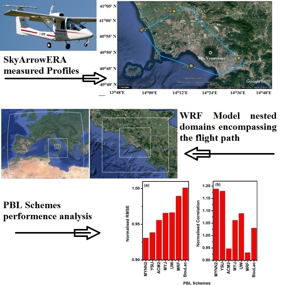
2. Materials and Methods

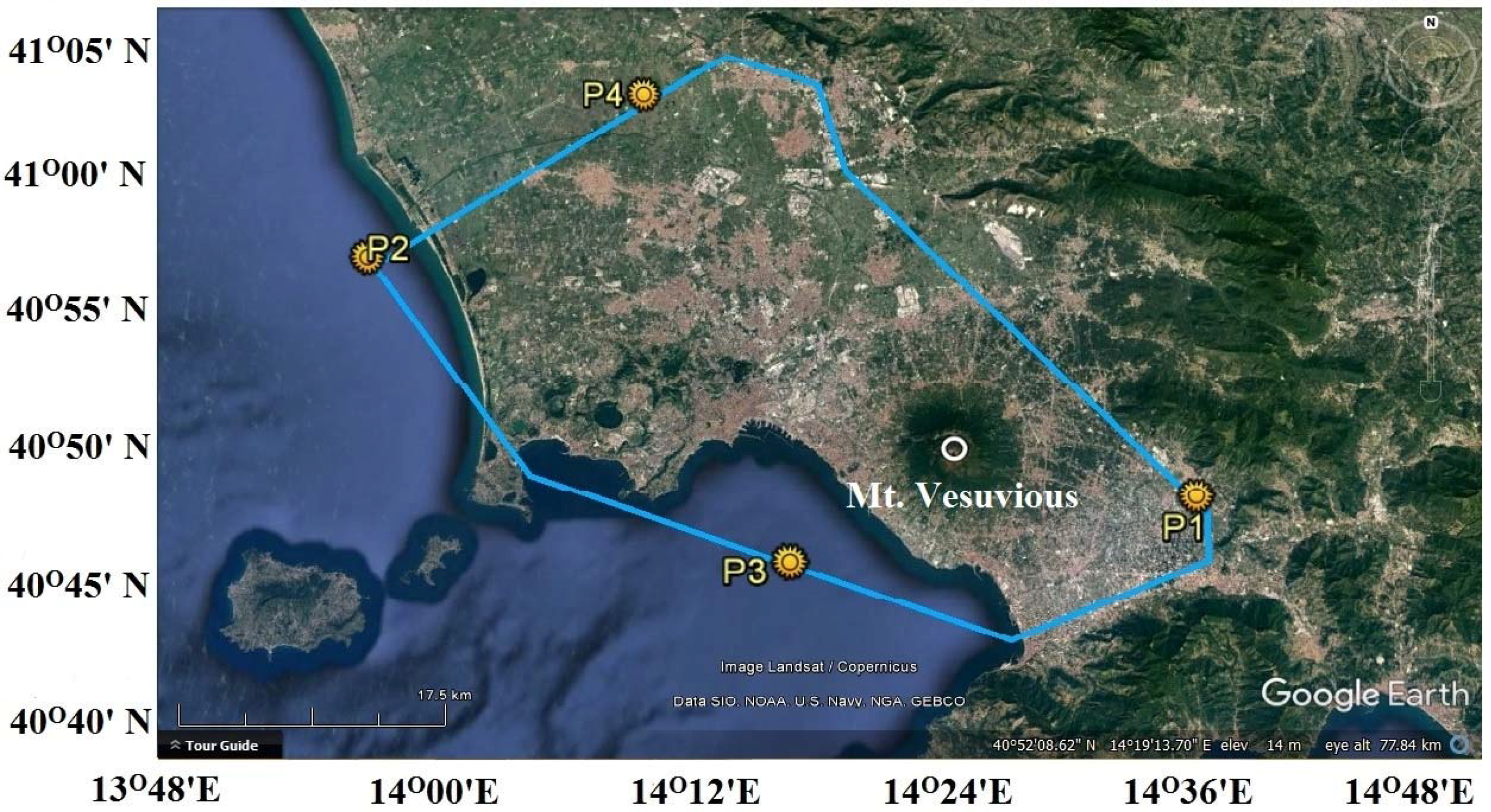
2.1. Study Area

Aircraft observations were performed over an area of circa 1300 km², situated in Campania region (Southern Italy) and roughly centered in the city of Naples (40°51′ N, 14°21′ E), which is bounded by the Appennini and anti-Appennini mountains to the east and southeast, and by Naples Bay and Tyrrhenian sea to south and west (Figure 1). The surface encompassed by flights is mainly made of flat land that is part of the two plains extending northwest of Naples and southeast of Mount Vesuvius and is surrounding the strip of conurbation that spreads from Naples to Caserta. This urban area is recognized as the largest metropolitan area in the Mediterranean Basin [28]; it is often affected by high pollution due to anthropogenic activities associated with calm and stagnant air masses, and its effect on health is a concern for the scientific community and policy makers [29,30,31,32].The remaining surface is occupied by agricultural land and small industrial districts [33].

The climate is typically Mediterranean, with mild winter providing most of the rainfall and a relatively dry and hot summer. Prevalent winds blow along the northeast to southwest direction, in a local breeze circulation pattern. The presence of Mount Vesuvius complicates this basic frame, since air masses are forced to move around its foothills, thus creating areas of relatively calm air downwind [33].

2.2. Aircraft Data

The Sky Arrow Environmental Research Aircraft (ERA) is a small airplane equipped with sensors to measure three-dimensional wind vectors (u, v, w), together with temperature, water vapor, trace gas concentrations, and other atmospheric parameters at high temporal frequency [14]. It has a cruise speed of 170 km/h and can fly up to a height of about 3000 m. The wind components are measured by means of a pressure sphere recording an airspeed velocity vector (e.g., relative to aircraft frame) that is post-processed to subtract aircraft motion, obtaining an absolute (i.e., relative to earth) wind vector following [34,35]. Details of the Sky Arrow ERA meteorological instrumentation relevant to this study is summarized in

Table 1. Details of meteorological instrumentation used during Sky Arrow Environmental Research Aircraft (ERA) flights.

Serial Number	Instrument	Parameters Measured	Accuracy
75H 0590	LICOR-7500-LI-COR/LI-COR Biosciences, Lincoln, NE, USA	CO2 and H–O densities of air	Within 1% of reading for CO2 and within 2% of reading for H2O
ATDD03-3	Best Aircraft Turbulence (BAT) probe/NOAA, Silver Spring, MD, USA; Airborne Research Australia, Adelaide, Austrilia	3D wind speed (u, v, w) with respect to aircraft	The ratio of standard deviation of w ~5%
LD90-3300HR	Riegl Laser Altimeter LD90-3/RIEGL Laser Measurement Systems GmbH, Horn, Austria	Aircraft flying height from the ground	Typically 0.5 m at highest range and 10 cm at minimum range
CM1480	C-MIGITS (Accelerometer)/Systron Donner Inertial, Concord, CA, USA	Position, velocity, and attitude information	Position (Spherical Error Probable-SEP): 3.9 m, Velocity (1 sigma, horiz/vert): 0.1/0.1 m/s, Pitch and roll (1 sigma): 1.0 mrad, Time mark output 1 pps: 1 microsecond, Heading (1 sigma, in motion): 1.5 mrad
2003-004	GPS OEM4 Family/Novatel, Calgary, AB, Canada	Position, velocity, altitude ASL (Above Sea Level) and GPS time	Position accuracy 1.8 m, velocity accuracy 0.03 RMS, time accuracy 20 ns RMS
Q03045	LI-190SA Photosynthetically Active Radiation (PAR)-Radiometer/LI-COR Biosciences, Lincoln, NE, USA	Photosynthetic photon flux density (PPFD)	Sensitivity: Typically 5 μA to 10 μA per 1000 μmol s−1 m−2 Linearity: Maximum deviation of 1% up to 10,000 μmol s−1 m−2

.

High-frequency (50 Hz) observational data streams were then block-averaged to obtain 4 s average values. The Sky Arrow performed five flights on 7–9 October 2014 (

Table 2. Aircraft flights and profiles details; the time of each profile is the average of the UTC time during the profile measurement interval, typically about 5 min to 15 min.

Serial Number	Flight	Date and Time	Profiles
1	Flight 1	7 October 2014, 08:39–10:58 UTC	1 (09:05 UTC), 2 (09:46 UTC), 3 (10:23 UTC), 4 (11:12 UTC)
2	Flight 2	7 October 2014, 12:38–16:56 UTC	1 (14:42 UTC), 2 (13:50 UTC), 3 (13:16 UTC), 4 (14:12 UTC)
3	Flight 3	8 October 2014, 12:47–14:46 UTC	1 (13:09 UTC), 2 (14:11 UTC), 3 (14:39 UTC), 4 (13:45 UTC)
4	Flight 4	9 October 2014, 08:39–10:37 UTC	1 (08:56 UTC), 2 (09:36 UTC), 3 (10:06 UTC), 4 (10:55 UTC)
5	Flight 5	9 October 2014, 12:09–14:24 UTC	1(14:19 UTC), 2 (13:17 UTC), 3 (12:46 UTC), 4 (13:40 UTC)

). The flight track was designed as a box encompassing inland and sea horizontal transects, with a vertical sounding profile on each of the four corners (Figure 1): Profile 1 (referred as PRF1 hereafter) at (40°47′39.35″ N, 14°37′52.82″ E) and Profile 4 (referred as PRF4 hereafter) at (41°04′22.49″ N, 14°10′06.27″ E) were obtained over land, while Profile 2 (referred as PRF2 hereafter) at (40°57′05.68″ N, 13°56′19.41″ E) and Profile 3 (referred as PRF3 hereafter) at (40°45′12.89″ N, 14°18′00.54″ E) were made over the sea. On PRF1 to PRF4, the aircraft flew a vertical profile from the minimum safety height (~150 m) up to the free troposphere (~2000 m above land and ~1000 m above sea), both upward and downward, performing spirals with about a 1.5-km diameter. Profiles of wind speed, wind direction, air temperature, and specific humidity were obtained by extracting ascending and descending legs from the flight paths for the subsequent comparison with model data.

2.3. Meteorological Model

The Advanced Research Weather Research and Forecasting model (WRF-ARW) version 3.5.1 has been configured with four nested domains, keeping the outermost domain at the continental scale, and the inner domains at the national and local scales (Figure 2).

The model domains use a grid of 3 km × 3 km resolution in Domain 3, and a 1 km × 1 km resolution in the innermost domain, i.e., Domain 4, with 41 vertical levels stacked closest near the ground, and approximately 11 vertical levels below 1 km above-ground level. WRF simulations have been driven by National Oceanic and Atmospheric Administration (NOAA)/National Centre for Environmental Prediction (NCEP)-Global Forecast System (GFS) global scale meteorological forecast with a horizontal spatial resolution of one degree and with time resolution of 3 h. The dynamics and physics schemes used by WRF forecast are resumed in

Table 3. Overview of WRF model configuration presently used for the Air quality in Salerno and Napoli districts (AriaSaNa) project. PBL: planetary boundary layer.

Dynamics	Non Hydrostatic
Data	NCEP GFS
Interval	3 h
Gridsize and Resolution	Domain1: (80×57) × 34: 27km × 27km Domain2: (95× 95) ×34: 9km × 9km Domain3: (69× 69) × 34: 3km × 3km Domain4: (69× 69) × 34: 1km × 1km
Map projection	Lambert Conformal
Horizontalgrid system	Arakawa-C grid
Integration time step	225 s
Vertical coordinates	Terrain-following hydrostatic pressure vertical co-ordinate with 34 vertical levels
Time integrationscheme	Third order Runga–Kutta Scheme
Spatialdifferencingscheme	Sixth order center differencing
Land surface option	Noah land surface scheme
Microphysics	WSM six-class graupelscheme
Shortwaveradiation	(old) Goddardshortwavescheme
Longwaveradiation	Rapid Radiative Transfer Model (RRTM) scheme
Cumulus parameterization	Kain–Fritsch scheme in Domain 1 and 2 and no scheme in Domain 3 and 4
Surface layer physics	Monin–Obukhovsimilaritytheory
PBL schemes tested in present work	ACM2, BouLac, MRF, MYJ, MYNN2, UW, YSU

.

Surface model results depend on the proper definition of land cover and soil composition. The land cover description has been improved by the introduction of the European Coordination of Information on the Environment (CORINE) land cover at 250-m resolution (http://land.copernicus.eu), while no information was available to enhance the soil composition description with respect to the standard worldwide WRF database.

The WRF ARW version 3.5.1 has 13 PBL schemes [36], which can be mainly grouped based on Richardson Number (Ri) or turbulent kinetic energy (TKE) criterion, which is commonly referred as first-order closure and TKE closure schemes [16] for PBL turbulence modeling and PBL height determination. PBL height is considered as the vertical limit where heat, moisture, and momentum are mixed in NWP models [37], affecting the reconstruction of dispersion and ground concentrations of various pollutants [2]. Different PBL schemes use different criteria to estimate PBL height, but the choice of the specific PBL scheme to be implemented is often made arbitrarily. Performance analysis of PBL parameterizations has been reported for specific regions in the last decade [15,16,19,21,22,23,24].

For the present study, three first-order closure PBL schemes (ACM2; MRF; YSU) and four TKE closure schemes (MYJ; UW; MYNN2; BouLac) have been chosen, based on the findings of previous studies [21,22,25,26]. A brief description and physical working principle of each of the chosen scheme is given hereunder.

2.3.1. The Asymmetrical Convective Model Version 2 (ACM2) Scheme

ACM2 is a first-order, non-local closure scheme [38] that was obtained as a modification of the ACM1 scheme of the MM5 model, which was derived from the Black adar scheme [39]. The scheme has an eddy-diffusion component, in addition to the explicit non-local transport of ACM1.

The non-local mixing term dominates the local mixing term through most of the depth of the convective PBL, but the local mixing term can be larger near the top of the PBL where the wind shear might be greater. The non-local transport term is set to zero, and local closure is used in stable conditions [26]. The scheme is found to have high accuracy in reproducing the vertical profiles of velocity and potential temperature by considering non-local and local closure for vertical mixing together [38]. ACM2 determines PBL height where the bulk Richardson number (Rib) exceeds a threshold value of 0.25.

2.3.2. Medium-Range Forecast (MRF) Scheme

MRF is a non-local first-order closure scheme [40] that incorporates a counter-gradient correction term into down-gradient diffusion defined by local mixing only [41]. Compared to local schemes, MRF showed higher accuracy in simulating the deeper mixing within unstable PBL, where larger eddies entrain higher potential temperatures above the PBL into the PBL [42,43]. The PBL height is calculated iteratively where Rib exceeds a threshold value of 0.50.

2.3.3. Yonsei University (YSU) Scheme

YSU is a first-order, non-local scheme [44]. It comes after a modification from the MRF scheme [40] of the MM5 model [21]. It uses a parabolic K-profile in an unstable mixed layer with the addition of an explicit term to treat the entrainment layer at the top of the PBL [22]. The buoyancy-driven PBLs with shallower mixing in strong-wind regimes are better simulated by YSU compared to MRF [26,44]. YSU determines PBL height where Rib exceeds a threshold value of 0.

2.3.4. Mellor–Yamada–Janjic (MYJ) Scheme

The classification of the Mellor–Yamada (MY) family schemes can be understood as “simplified second-order closure” [45], which is often indicated as “1.5-order” because they implement a reduced set of second-order moment equations [46]. The term “1.5-order” usually means a first-order closure with eddy viscosity K-coefficients dependent on TKE, which in turn is calculated from a budget equation. MY Level 3 and higher use a full set of second-moment budgets with proper closure hypotheses simplified by a scale analysis based on a departure from isotropy metric and the application of the so-called “boundary layer approximation” to obtain simpler models. The widely-used MY Level 2.5 model is based on the solution of the TKE budget equation only, and is usually indicated as a “1.5 order”. The MYJ scheme comes after modification from the MM5 model’s ETA scheme [47]. It solves a prognostic equation for TKE with a diagnostic estimation of potential temperature, water vapor variance, and covariances [48]. The scheme is considered to improve the Mellor–Yamada Level 2.5 local scheme [49,50] without particularly large computational expense [26]. It determines PBL height by the level where TKE decreases to a prescribed small value (0.2 m² s⁻²).

2.3.5. Mellor–Yamada–Nakanishi–Niino Level 2.5 (MYNN2) Scheme

MYNN2 also comes under MY family scheme, which can be termed as a “simplified second order” [45]. It is a variation of the Mellor–Yamada Level 2.5 scheme [49,50], which uses liquid water potential temperature and total water content as the thermodynamic variables. It also takes into account the effects of buoyancy in the diagnosis of the pressure covariance terms, and uses closure constants in the stability functions and mixing length formulations that are based on large eddy simulation (LES) results instead of observational datasets [48]. Furthermore, the MYNN2 model considers the effect of stability on the turbulent length scale, obtaining a mixing length formulation that is considered more flexible across the stability spectrum compared to MYJ [51,52,53]. MYNN2 determines PBL height, where the TKE falls below a critical value of 1.0 × 10⁻⁶ m² s⁻² [21].

2.3.6. Bougeault–Lacarrere (BouLac) Scheme

BouLac is a 1.5-order, local closure scheme [54] with a TKE prediction formulation designed to extend PBL turbulence parameterizations to orography-induced turbulence and, within WRF, to be used with the Building Environment Parameterization multi-layer, urban canopy model [55]. The BouLac scheme has been found to better represent the PBL in regimes of higher static stability compared to non-local schemes [16]. PBL height determination with this scheme is achieved at a level where prognostic TKE reaches a sufficiently small value (e.g., 0.005 m² s⁻²).

2.3.7. University of Washington (UW) Scheme

The UW scheme is a 1.5-order, local TKE closure scheme [56,57,58]. The UW scheme has been originally developed for climate modeling application. It uses moist-conserved variables, TKE as a diagnostic rather than a prognostic variable, and an explicit entrainment closure to diagnose effective entrainment diffusivity at the edge of convective layers [57]. UW has been found to better reproduce the night-time stable boundary layer and sub-stratocumulus layers. PBL height determination by UW scheme is based on the Rib threshold (0.25) used in all cases of stability.

The applicability of the previously listed PBL parameterizations in a non-hydrostatic model at 1-km grid spacing could be considered questionable because the mentioned space resolution falls within the so-called “Terra Incognita” zone [59,60]. Nonetheless, it is common practice to apply WRF and other non-hydrostatic models down to 1-km grid spacing for regional to urban scale applications. This is generally considered acceptable, even if we should keep into account that the daily convective eddies can have a size of the order of the horizontal grid spacing, and could be partially resolved. The effective spatial resolution of WRF that has been evaluated by Skamarock [61] to be of the order of 7 dx, should anyway tend to guarantee that PBL parameterizations can still be considered reliable at 1-km grid spacing.

2.4. Model Performance Assessment

The model-simulated air temperature, specific humidity, wind speed, and wind direction obtained by different PBL parameterization simulations were directly compared to observational data collected by the Sky Arrow. WRF-ARW outputs have been stored with hourly frequency. The simulated vertical profiles of meteorological variables have been extracted at the corresponding aircraft profile locations, selecting the nearest available time frame and applying bilinear interpolation among the four surrounding grid points on each model level. PBL height obtained from the model as a diagnostic parameter is also compared with the PBL height obtained from the vertical profile soundings of the aircraft. The observed PBL heights are subjectively estimated by visualizing the profiles of potential temperature and water vapor [62]. By applying the potential temperature profile criterion, which is indicating atmospheric static stability, the PBL height can be taken as the level where maximum gradient occurs. In case of water vapor profiles, the PBL height is taken as the level of the minimum vertical gradient, with a noteworthy reduction in atmospheric moisture [63]. We have also validated our results of PBL height values by using bulk Richardson number criterion [64]. The results have been statistically analyzed using root mean square error (RMSE) and Pearson correlation (r). Model results were extracted from the innermost domain (1-km grid-spacing domain), horizontally interpolating model results to measurement points and time. The RMSE has been defined as follows:

$$\mathrm{RMSE}=\sqrt{\frac{1}{N}{\displaystyle \sum _{i=1}^N{\left(M_i-O_i\right)}^2}}$$

And Pearson correlation (r) has been calculated as:

$$r=\frac{{\displaystyle \sum _{i=1}^N\left(M_i-{\overline{M}}_i\right)\left(O_i-{\overline{O}}_i\right)}}{\sqrt{{\displaystyle {\sum }_{i=1}^N{\left(M_i-{\overline{M}}_i\right)}^2\sqrt{{\displaystyle {\sum }_{i=1}^N{\left(O_i-{\overline{O}}_i\right)}^2}}}}}$$

where M_i = model-simulated values, O_i = observed values, and N = number of points.

Statistical parameters were also averaged across multiple flights performed over the sea, over inland areas, in the morning and the afternoon. This was done to assess the importance of the error variability related to geographical features (i.e., sea versus land) or to meteorological conditions (i.e., morning versus afternoon flights) with respect to error variability related to the different PBL schemes under investigation.

In order to compute an empirical total performance index integrating the performance of each PBL scheme on all of the flights and for all of the examined variables, RMSE and r were at first computed for all of the flights, obtaining one value for each variable; then, these values were normalized over the average of all of the PBL schemes, and finally averaged for all of the variables. Normalized RMSE and r were then obtained in a way that the mean of all of the schemes is equal to one.

3. Results and Discussion

Measurements of meteorological parameters (air temperature, specific humidity, wind speed, and wind direction) from all profiles of Sky Arrow flights were compared with the corresponding WRF output. It is worth mentioning that the comparison of model results with high-frequency aircraft measurements recorded inside the boundary layer is not a straightforward and consolidated practice. The model based on Reynolds-averaged Navier–Stokes (RANS) equations provide results that are representative of the space and time averages of the meteorological variables. The effective space and time resolution of WRF depends on the computational domain grid spacing and the numerical advection scheme [61], and it is the usual practice to compare the results of model simulation with grid spacing of a few kilometers with the observed variables’ time averages of the order of 1 h, implicitly assuming that the averaging time window is large enough to sample the whole boundary layer turbulence spectrum. This approach cannot be applied to local scale PBL airborne measurements due to the speed of the aircraft. Short time window averages do not completely filter out PBL turbulence, especially in neutral to convective conditions. Therefore, we should expect observations to include short wavelength fluctuations and possibly transient structures that cannot be reproduced by model simulations. Moreover, shallow layers characterized by relevant specific humidity variations are expected to be removed by buoyancy over timescales that are comparable with the average values and representative of model results. Nevertheless, the strategy adopted here, e.g., treating measured profiles as quasi-instantaneous representations of vertical atmospheric variability and comparing them with the model output interpolated at the time of the measurements, is only capable of giving observational evidence of atmospheric properties, and is commonly adopted whenever comparing aircraft in-situ measurements with model data.

The model performance is analyzed for each variable on multiple profiles over different areas of the innermost domain (i.e., sea versus inland) and at different times of the day (i.e., morning versus afternoon). The results are reported at the single profile detail level only for one flight (Flight 3), which is quite representative of the encountered conditions during the three days of the campaign. Afterwards, aggregated performance indexes considering all of the profiles of all of the flights are presented and discussed.

3.1. Synoptic and Local Circulation Conditions during Flights

To understand the synoptic weather situations during the aircraft observational period, we have analyzed the surface pressure charts showing pressure and weather fronts at 00:00 UTC on 8–10 October 2014 provided by the Met Office (available at http://www.wetterzentrale.de), and the thickness isopleths for the layer (500–1000) hPa (dam) and temperature at 850 hPa (°C) at 00:00 UTC of 8–10 October 2014 provided by European Centre for Medium Range Weather Forecast (ECMWF) reanalysis (ERA-Interim) (available at http://www.meteociel.fr).

Weather conditions for the measurement period (7–9 October 2014) showed a reinforcing high pressure system over northeastern Africa extending northeastward and linking to the Blocking Highs over Russia while a deeply cyclonic vortex persisted over the United Kingdom (UK) and much of the North Atlantic area, with the polar front jet stream forced way south across the Atlantic toward northwestern Africa before returning northeastward across the western Mediterranean Basin and Central Europe (Figure 3 panel a-b-c). These complicated patterns lead to an increasingly warm southwesterly flow over the study area, with temperatures rising well above average and higher than average stability conditions for the season (Figure 3 panel a1-b1-c1).

The limited pressure gradient that occurred over southern Italy favored the development of a sea breeze circulation characterized by surface winds blowing from S–SW during the daytime and N–NE during the night-time over the Naples region. Local meteorological conditions are described by the observations of the Napoli Capodichino airport meteorological station (International Civil Aviation Organization (ICAO) code LIRN) reported in Figure 4. The pressure shows high values with a slowly growing trend during 7–8 October 2014 becoming stationary from 8 October 2014 onward. The daily variability of wind speed and direction has a cyclic structure that characterizes coastal breeze circulation. Daily maximum wind speeds ranging between 3 m s⁻¹ and 4 m s⁻¹ are recorded during the early afternoon, and associated with directions from S–SW, while weak nightly currents blow from N–NE. These directions are determined by the gulf of Naples’ local circulation. The temperature and relative humidity daily cycles are quite regular, with a slight growing trend of daytime maximum temperature, confirming the absence of relevant cloudiness.

WRF simulations were able to satisfactorily reconstruct the main features of the near surface meteorological variables with all of the tested PBL parameterizations. Figure 4 shows the results of WRF run with the MYNN2 scheme, which resulted as the best performing, with a correct reconstruction of all of the variables except for a tendency to overestimate night-time minimum temperature and surface pressure during the last day. The coastal breeze wind speed and direction cycle is particularly nicely reconstructed (Figure 4b). The results obtained with the different PBL schemes were hardly distinguishable when superposed in the same figure, except for MYJ, which showed an overestimation of daytime maximum wind speed with an overall BIAS = 0.19 m s⁻¹.BIAS, RMSE, and correlation obtained with the different PBL schemes ranged within the following intervals: wind speed: BIAS = −0.19–0.19 m s⁻¹; RMSE = 0.54–0.68 m s⁻¹; r = 0.77–0.86; temperature: BIAS = 0.66–1.06 K; RMSE = 1.21–1.39 K; r = 0.95–0.96; relative humidity: BIAS = (−3.36)–(−0.39)%; RMSE = (5.09–7.09)%; r = 0.86–0.93.The comparison of WRF results with surface observations confirms the capability of the model to describe the circulation structure during coastal breeze conditions over the investigated area, as it has been already verified during different midsummer episodes by Finardi et al. [11].

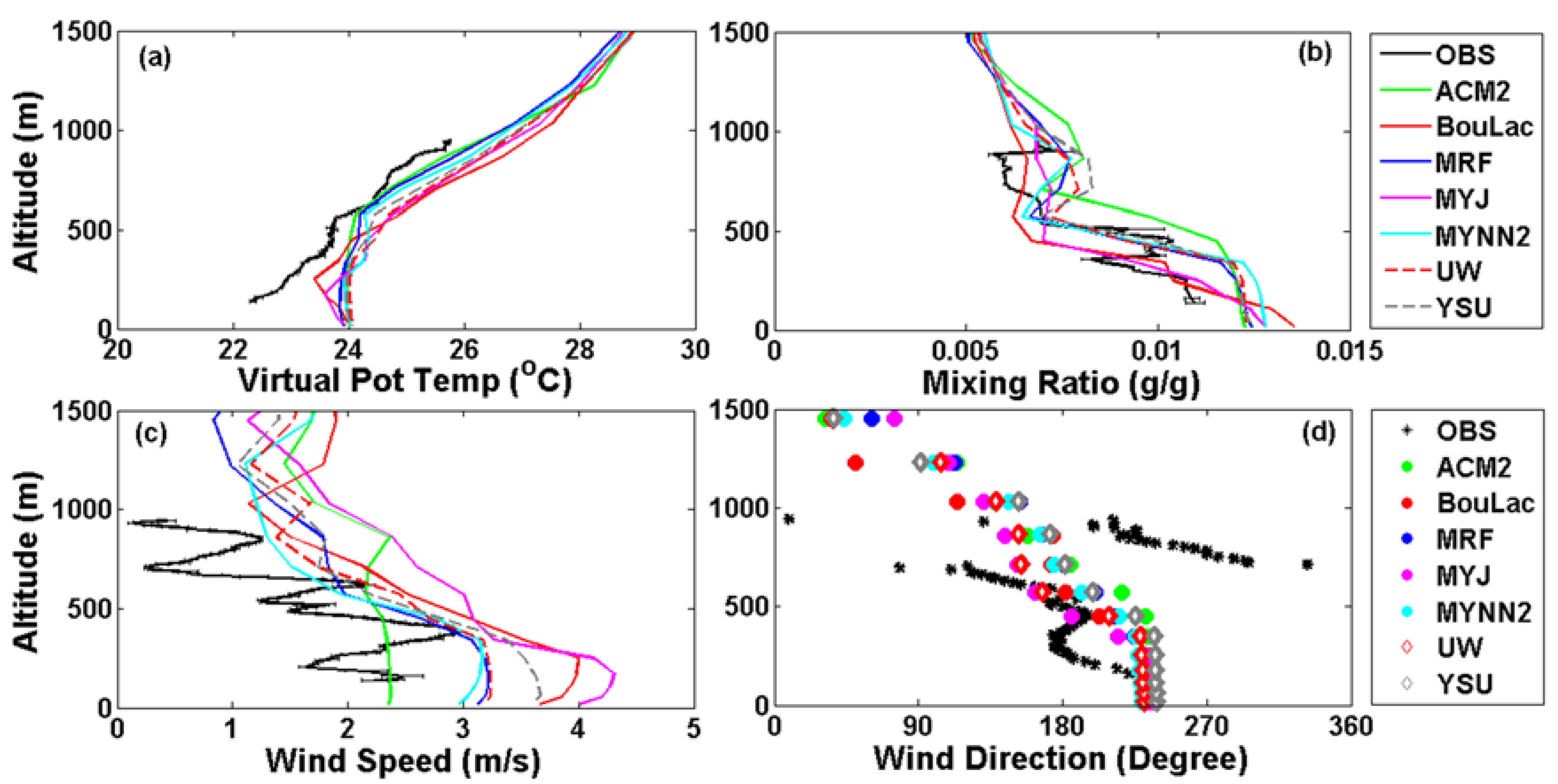
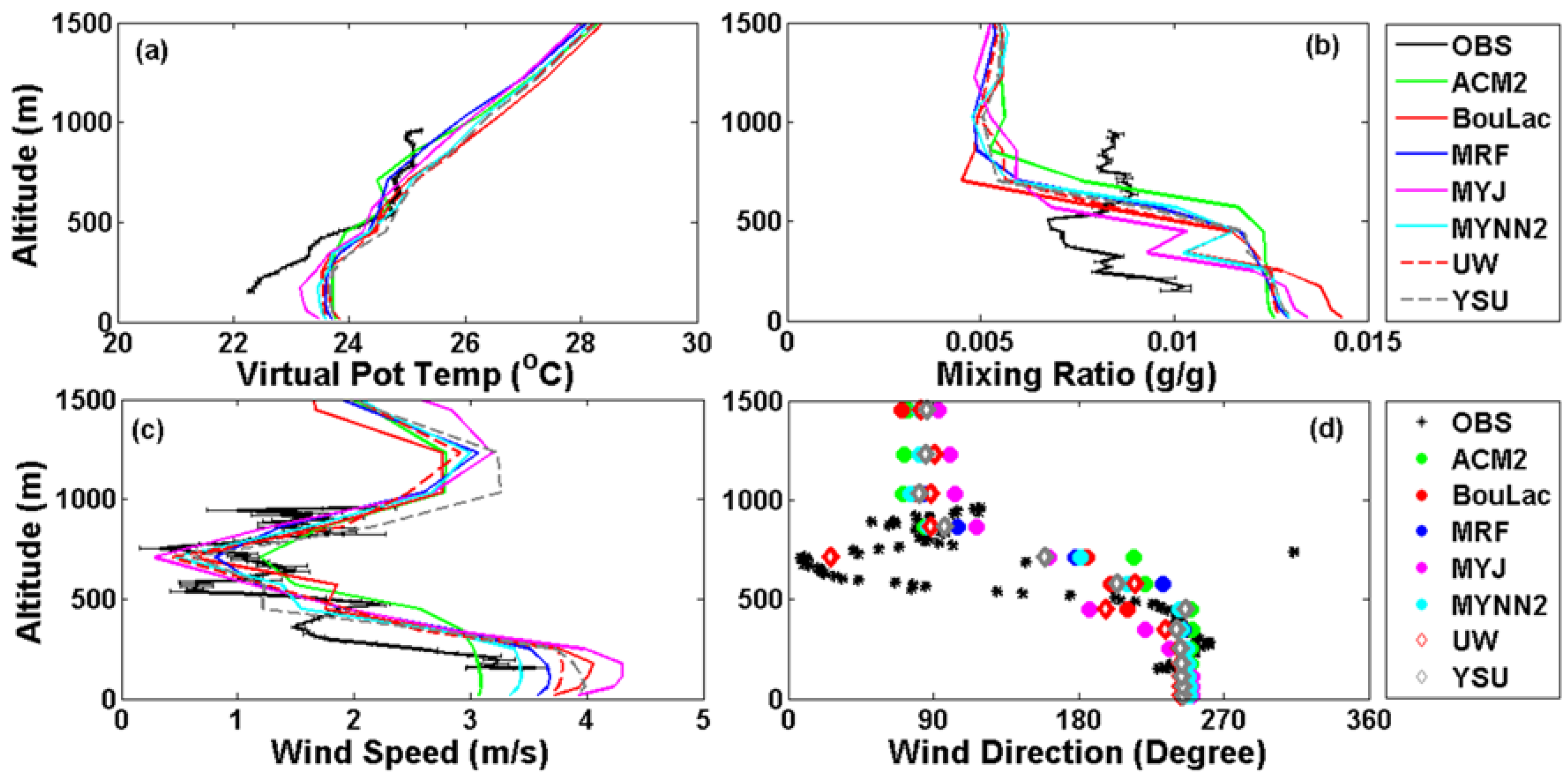
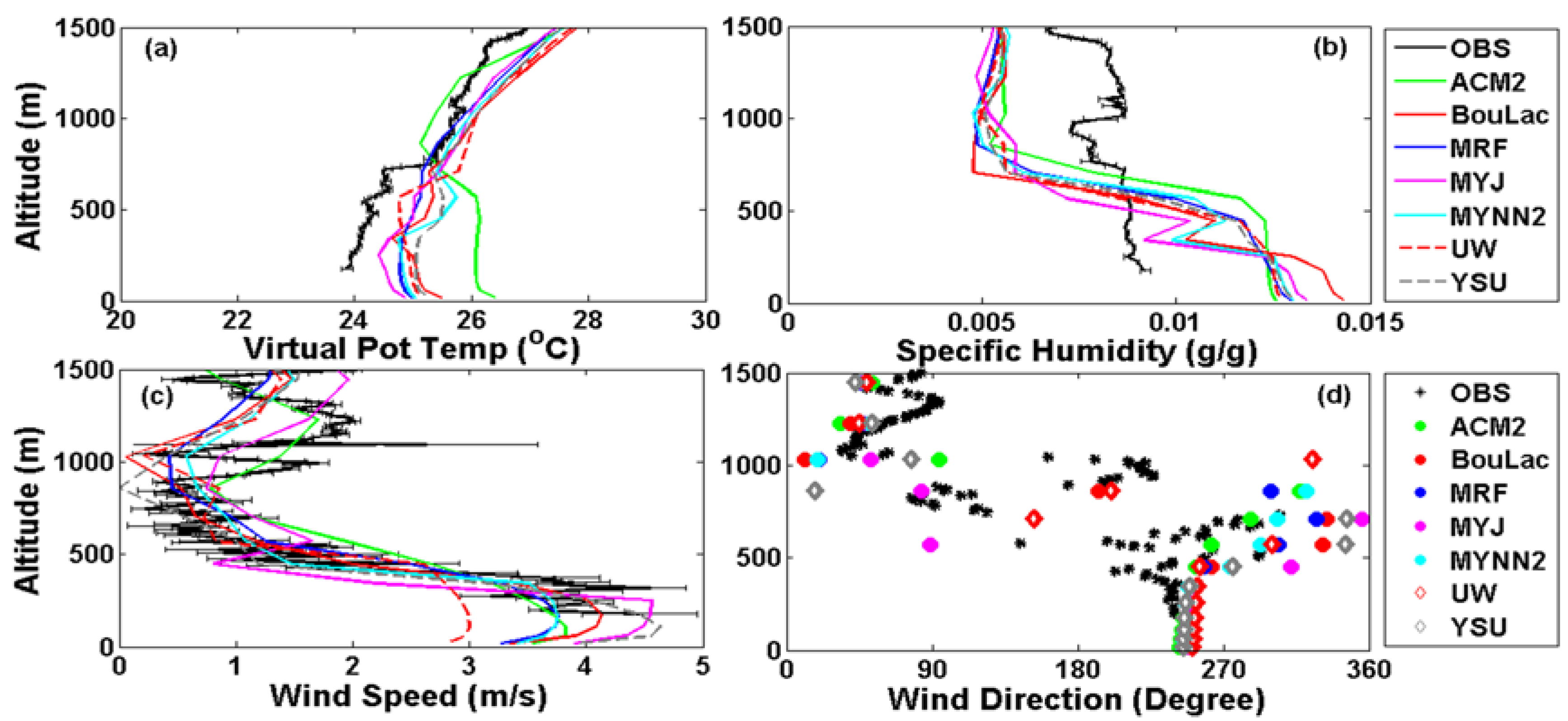
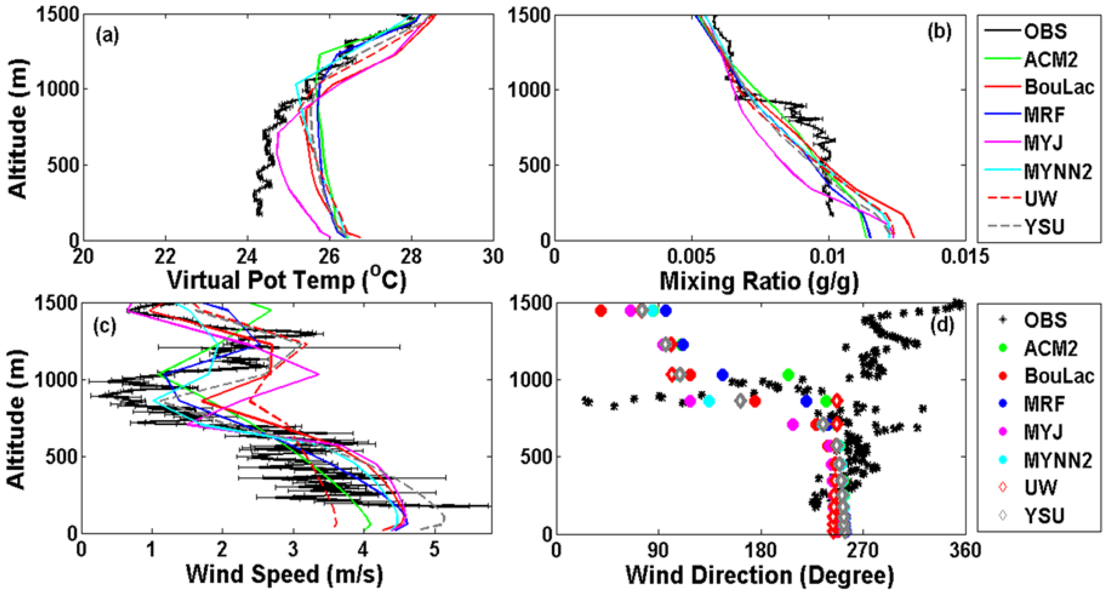
3.2. Vertical Profiles of Air Temperature, Specific Humidity, Wind Speed, and Direction

To get insights regarding the chosen PBL schemes with respect to observations, we have selected Flight 3 profiles in the present work. As mentioned earlier, Profile 1 (Figure 5) is overland, whereas Profile 2 (Figure 6) and 3 (Figure 7) are over sea, and Profile 4 (Figure 8) is again over land. The overall comparison shows that the main features of the vertical layering of the atmosphere are captured by WRF simulations with all of the considered PBL schemes. The wind speed is everywhere decreasing with height, with a SW direction near the surface and a strong shear in both direction and speed between 500–1000 m agl. Weak winds are observed from NE–SE in the upper monitored layers. The development of the modeled boundary layer matches the vertical location of the major temperature gradient, and correctly reproduced the upper layer temperature slopes. This generally indicates a reasonable reconstruction of the PBL depth and its time variation, even if the virtual potential temperature is generally overestimated in the lower atmospheric layers located within the PBL. It is worthwhile to remember that the growth of the PBL is not monotonic over land due to the development of the thermal internal boundary layer, which follows the sea breeze front penetration.

Some peculiar features of the observations are not reproduced by WRF with any of the PBL parameterizations. The measured virtual potential temperature shows a stable slope within the boundary layer that is particularly evident over sea (Figure 6 and Figure 7), while modeled profiles are nearly uniform within the PBL, as expectable in well-mixed conditions. The specific humidity is overestimated in the lower layers and underestimated in the upper layers at Profile 1 and 3 (Figure 5 and Figure 7), where observations show limited variation with height and relatively high values in the upper layers with respect to the other measured profiles. No model simulation is capable of reproducing the NW wind direction that is detected by measurements at Profile 4 (Figure 8), which is at variance with all of the other profiles measuring winds from directions around E, as predicted by the models. These discrepancies can be attributed to local features that are possibly transient, and are connected to the development to the breeze cell circulation and in particular, to the return current aloft. It can be noticed that WRF predicts a higher specific humidity over the sea than over land within the boundary layer, while measurements show variable conditions without clear sea/land differences. This behavior can be attributed to the near-coast location of the profiles measured over the sea.

Looking in more detail at the differences shown by the WRF results with the different PBL schemes, it can be observed that at the PRF1 inland vertical profile (Figure 5a), all of the schemes are overlapping each other in the lowest 600 m, and they all overestimate measured values of less than 1 °C. ACM2 shows a different vertical profile and a larger overestimation of the order of 2 °C. The observed (OBS) air virtual potential temperature between 600–1000 m is warmer than in the lower layers, and is roughly coincident with the model-simulated profiles. Only ACM2 shows temperatures colder than the measurements in this layer. All of the schemes’ results are coincident above 1000 m, where they overestimate measurements of less than 1 °C, reproducing its vertical slope. The model reproduction of the vertical variation of wind is correct, showing the relevant decrease of wind speed and wind direction rotation in the shear layer observed between 500–900 m (Figure 5c,d). The trend of wind profiles near to the surface is better reproduced by ACM2 and MYNN2, while also MRF and BouLac schemes are able to reproduce the observed profile to a good extent. UW underestimates near surface winds, while MYJ and YSU overestimate them. The virtual potential temperature measured by PRF2 over sea (Figure 6a) is well reproduced by all of the schemes, with MYJ and BouLac showing the largest overestimation above 500 m agl, but being nearest to the observations in the lower layers. The observed wind speed profile (Figure 6c) shows generally weak winds, with a strong vertical variability and many pockets of high wind speed at 200 m, 400 m, 650 m, and 850 m. These features, which are not reproduced by simulations, make it difficult to rank the performances of the different PBL schemes. However, it can be argued that MYNN2, MRF, and UW perform better than the other schemes, while MYJ, BouLac, and YSU overestimate wind speed, and ACM2 underestimates it. The vertical profile of the wind speed observed at PRF3 above sea (Figure 7c) is correctly described by WRF with all of the PBL schemes. MYNN2, ACM2, and MRF produce wind speed that is better comparable with values measured below 200 m, while all of the other schemes show a tendency to overestimate them, which is particularly pronounced for MYJ, BouLac, and YSU.

The detailed comparison of the different PBL schemes’ performance with virtual potential temperature measured at PRF4 above land (Figure 8a) show similar results in the lower 1000 m for all parameterization, while MYJ is closer to the measurements. On the other hand, MYJ and BouLac show larger errors over 1000 m, where MRF, ACM2, and MYNN2 better fit the virtual potential temperature measurements. MYJ shows also larger discrepancies than the other schemes with respect to specific humidity below 1000 m (Figure 8b). Wind speed (Figure 8c) observations are quite fluctuating along the entire profile, which is a feature that makes their comparison with model results difficult. The observed fluctuations must be considered a subgrid variation considering both horizontal and vertical resolution. The overall variation of wind speed with height is reproduced by almost all of the PBL schemes, with ACM2, MYNN2, and MRF performing best, and the tendency of YSU to overestimate near surface wind speed.

Model and data compared at different locations within the same area in the central hours of the day flight (Flight 3) show a highly dynamic situation, with a non-uniform sea breeze penetration and the presence of circulation layers: the southern profiles of the domain, PRF1 over land and PRF3 over sea(Figure 5 and Figure 7), both show a strong return flow with a wind turning from westerly (up to 700 m) to easterly (above 700 m) direction, which is correctly reproduced by all of the schemes. The northern profiles, PRF4 over land and PRF2 over sea, show a stronger sea breeze penetration (Figure 6 and Figure 8) that is not entirely reproduced by WRF, as a likely consequence of a non-optimal simulation of the timing of sea breeze penetration in a dynamic context. The complexity of the atmospheric flow and the PBL structure during sea breeze inland penetration is illustrated in Figure 9 by the results of WRF simulations on 8 October 2014 at 13:00 GMT with MYNN2 and YSU schemes. The sea breeze front is clearly detectable where the wind speed gradient is located just upwind of the maximum value of the PBL height. The overlap of the flight track helps to realize the intrinsic difficulty to compare local profiles with modeled atmospheric fields characterized by relevant space and time variability.

Overall, a larger variability among the schemes is observed for the wind vector than for temperature and specific humidity, while the observed and modeled variability among schemes is always lower than the variability among the different profiles for all of the variables. The observed and modeled profiles of air temperature, specific humidity, winds, and PBL height from flights 1, 2, 4, and 5 (not shown here) have also been analyzed, revealing similar behavior of the various schemes in reproducing atmospheric circulations, with respect to Flight 3 reported above (Figure 5, Figure 6, Figure 7 and Figure 8). Performance across the full set of flights is analyzed in the following section.

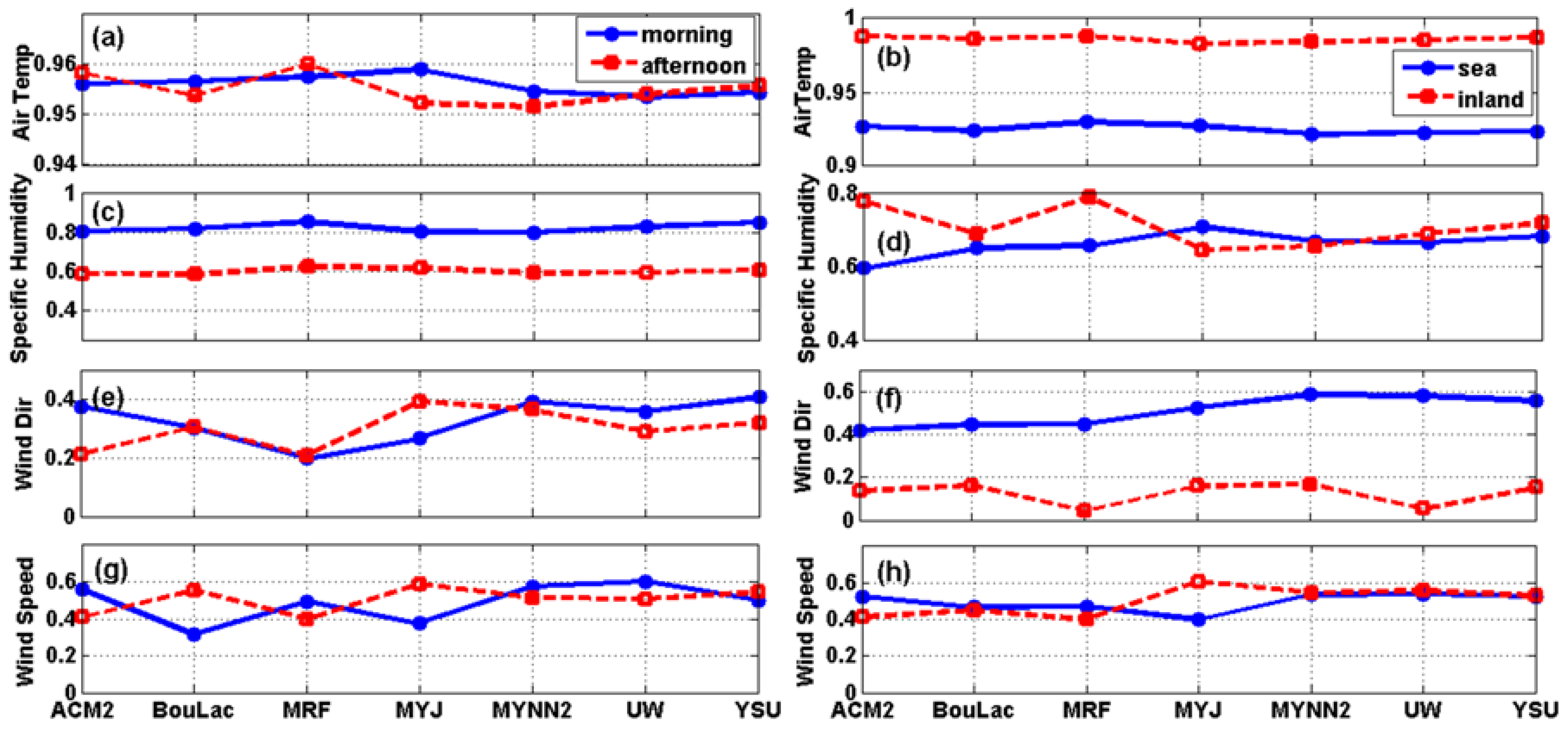
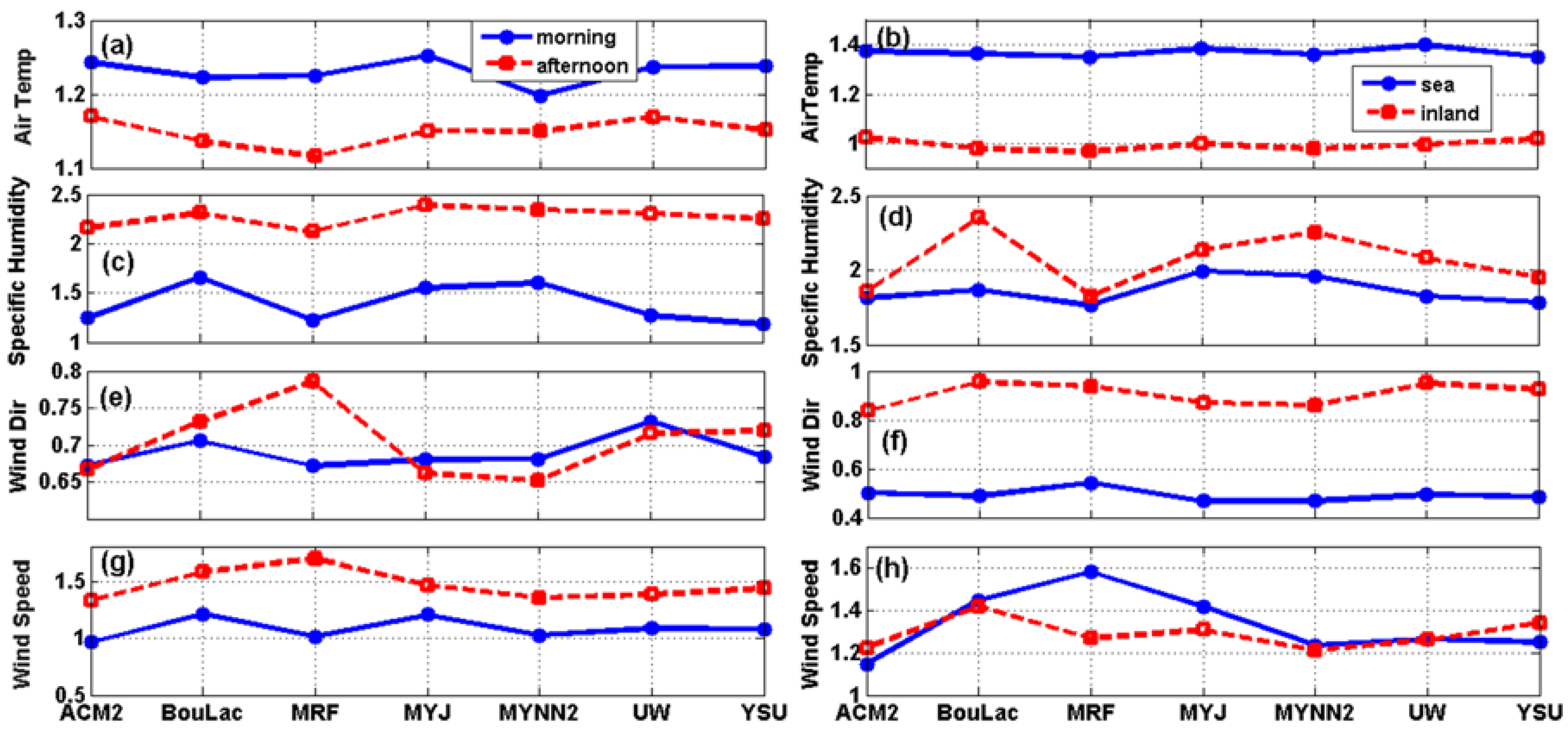
3.3. Spatial and Temporal Assessment of Model PBL Schemes

When grouping the observed profiles for all of the flights with respect to their location (i.e., over the sea or over the inland, Figure 1), and with respect the time of the day (i.e., morning or afternoon flights, Table 2), significantly better performance is overall achieved at inland sites with respect to the sea, and at morning with respect to afternoon flights (Figure 10 and Figure 11). However, important differences are observed among the variables: higher correlation coefficients and lower RMSE are obtained especially for specific humidity and temperature (Figure 10a,d and Figure 11a,d). For specific humidity analysis, it is observed that RMSE is lower during morning flights and over sea flights compared to those in the afternoon or over land. The wind direction (in degree) (Figure 10e,f and Figure 11e,f), shows better simulated profiles over sea, whereas afternoon and morning simulations perform similarly. Wind speeds are better simulated in the morning compared to the afternoon (Figure 10g,h and Figure 11g,h). The reasons for this difference in performance is likely related to difficulty in reproducing vertical variability at sea, where very shallow PBL develop that may not be entirely reproduced, as also confirmed by the detailed analysis of sea profiles from Flight 3 (Figure 5, Figure 6, Figure 7 and Figure 8). This result is also consistent with simulated PBL depths at sea locations that exhibit a larger bias with respect to observations at inland locations with well developed convective boundary layers (

Table 4. Performance statistics of PBL height prediction according to the seven configurations of PBL schemes for all of the profiles of the Sky Arrow flights. The best performances are highlighted in a bold red color, and the second best is highlighted in blue. Other values within ±60 m (1/2 of WRF grid spacing at 500 m) are reported in green. The profiles for which we cannot determine PBL height from observations are left blank in the OBS column.

Schemes	ACM2	BouLac	MRF	MYJ	MYNN2	UW	YSU	OBS
Profiles	Flight 1: 7 October 2014, 08:39–10:58 UTC
p1	1047	1040	912	995	1000	889	983	980
p2	586	671	601	628	528	439	517	700
p3	702	715	593	671	494	518	568	750
p4	1441	1390	1398	1435	1323	1392	1387	-
	Flight 2: 7 October 2014, 12:38–16:56 UTC
p1	1135	879	925	686	751	682	848	-
p2	770	630	871	743	762	694	773	450
p3	888	540	788	638	702	439	640	600
p4	1331	1142	1225	1017	1151	1159	1195	-
Flight 3: 8 October 2014, 12:47–14:46 UTC
p1	1002	901	850	744	705	830	949	1000
p2	464	390	382	356	364	425	418	360
p3	365	319	320	312	297	284	309	200
p4	972	859	799	790	877	1016	856	830
	Flight 4: 9 October 2014, 08:39–10:37 UTC
p1	421	445	302	392	347	403	390	400
p2	226	200	142	106	144	129	135	480
p3	128	183	161	145	141	138	147	500
p4	774	923	765	902	770	816	862	820
	Flight 5: 9 October 2014, 12:09–14:24 UTC
p1	654	653	441	472	381	557	449	1005
p2	268	198	240	203	201	190	204	400
p3	186	169	184	132	161	131	188	310
p4	770	754	614	446	538	670	570	680

).The reasons for the better performance at morning with respect to afternoon flights are likely related to the model capability of fully reproducing sea breeze development, and the interface between sea breeze and the synoptic circulation. Since inland profile locations PRF1 and PRF4 are relatively close to the coastal line, even relatively small errors in space and time in reproducing sea breeze penetration may lead to a significant bias in the model results (extracted at the requested point) with respect to observational values. Moreover, the model shows generally high values of specific humidity in the lower 500 m for profiles observed over the sea during all of the flights (Figure 5, Figure 6, Figure 7 and Figure 8).

BouLac, UW, MYNN2, and ACM2 proved to be the better schemes for simulating specific humidity profiles over land (Figure 10 and Figure 11). However, the overall variability between morning and afternoon flights, and between sea and inland profile sites, always exceeds the variability among different PBL schemes. This indicates the importance of the underlying meteorological model that overwhelms the importance of PBL scheme choice. YSU (first-order closure) and MYNN2 (TKE closure) are proved to be the best schemes for all of the profiles (Figure 12). Among the first-order closure schemes, YSU proved to be the best scheme for simulating the wind speed profiles of all of the flights. The MYNN2 scheme, which predicts TKE terms at subgrid levels, provided the best simulation overall, considering all of the meteorological variables and all of the observed profiles (Figure 12). MYNN2 uses a unique surface layer scheme, and was reported to better simulate surface heat fluxes (Banks et al. 2016) [22]. Madala et al. [19] also found that MYNN2 was better performing when compared against eddy covariance energy flux observations. MRF, YSU, and ACM2 have the ability of simulating deep convection/deep PBL in their formulation, which explains their relatively low performance over the sea, when compared with flight observations [26,48]. It has been observed [48] that MYJ produces a shallower PBL height than the non-local schemes during the daytime. The potential temperature profiles are showing a warm bias near the ground and a cool bias starting near 0.75 km and reaching above the PBL height by MYJ [48]. This might be the reason for the under performance of MYJ in the present study compared to MYNN2. MYNN2, UW, and BouLac showed improved reproduction of the observed profiles compared to other PBL schemes; however, the subtle difference in the base formulation results in the different performance of the three schemes. The UW is developed by taking into account stratocumulus clouds and their influence on PBL, and is therefore more suitable for climate runs with longer time steps, diagnosing rather than forecasting turbulent kinetic energy (TKE), and simulating layers determined by the vertically varying stability of the thermodynamic profile [26]. The BouLac scheme is better suited for cases with terrain-induced turbulence to study its impact on PBL [16]. It can be observed that the MYJ and MYNN2-simulated profiles for potential temperature, specific humidity, and wind speed are showing significant differences among each other, although the MYJ and MYNN2 base formulation is the same [49,50]. This can be explained by the difference in MYNN2 formulation constraints. It has been observed that MYJ is having a tendency to underestimate boundary layer height during upstream locations of convection, while MYNN2 improves this drawback over non-local PBL schemes and supports deep convection [48]. The mixing length formulations used in MYNN2 are also more flexible for the static stability regimes compared to MYJ [26]. This difference in formulation results in appreciable differences in the simulated profiles also in the present work (Figure 5, Figure 6, Figure 7 and Figure 8). Over land (profiles 1 and 4), the MYNN2-simulated profiles are showing a better reproduction of observed profiles compared to MYJ. Also, the afternoon simulated profiles show an improvement of MYNN2 compared to MYJ (Figure 10 and Figure 11) for all of the flights. It is worth noticing here that no modification on any of the PBL schemes used in the present study was made, keeping them in their original form, as provided in the WRF model.

As all of the profiles were observed during the day time when a surface heated convective boundary layer was already developed, it was possible for the TKE closure schemes to provide an overall good performance. It was found that the TKE closure schemes performed better than the first-order closure schemes for the CASES-99 experiment study over the Kansas area in the United States (U.S.) [16]. In our work, YSU performs better among first-order closure schemes. The YSU scheme increases the thermally-induced mixing and allows for the early development of PBL before noon, which is helpful for this scheme in comparison to ACM2 and MRF to better simulate the PBL height (Table 4). When we analyze the performance of TKE closure schemes, the MYNN2 scheme is ranked as the best in all of the flights and conditions (Figure 12).

The normalized RMSE and correlation values for Figure 12 are obtained using the ratio of RMSE/correlation value of a particular scheme divided by the mean value of all of the schemes. This normalization allows values to go above or below 1, as the average value (by considering all of the schemes) is lower/higher than an individual scheme value that is performing better/worse than the average. In case of normalized RMSE, MYNN2 is the best-performing scheme (Figure 12a), as the value of RMSE for MYNN2 is less than the average value calculated, which gives the lowest normalized RMSE value for MYNN2. Similarly, Figure 12b shows that MYNN2 again is having the highest correlation (greater than one in this case), which is a result of normalization.

However, our findings do not allow for the identification of a specific scheme providing a better performance in any condition. As evidenced by the discussion of WRF results at each measured profile location, the variability in model errors is more related to both the spatial and temporal variability of atmospheric properties than to the behavior of the different PBL schemes. Overall, our findings are consistent with Gioli et al. [65], indicating that sea breeze transition is a critical phenomenon to be correctly simulated in time and space with a WRF-based modeling setup. However, these results allow the identification of a subset of PBL schemes that perform comparably, and constitute useful data to constrain the choice of the PBL scheme in the setup of a WRF modeling chain for meteorological or air quality predictions.

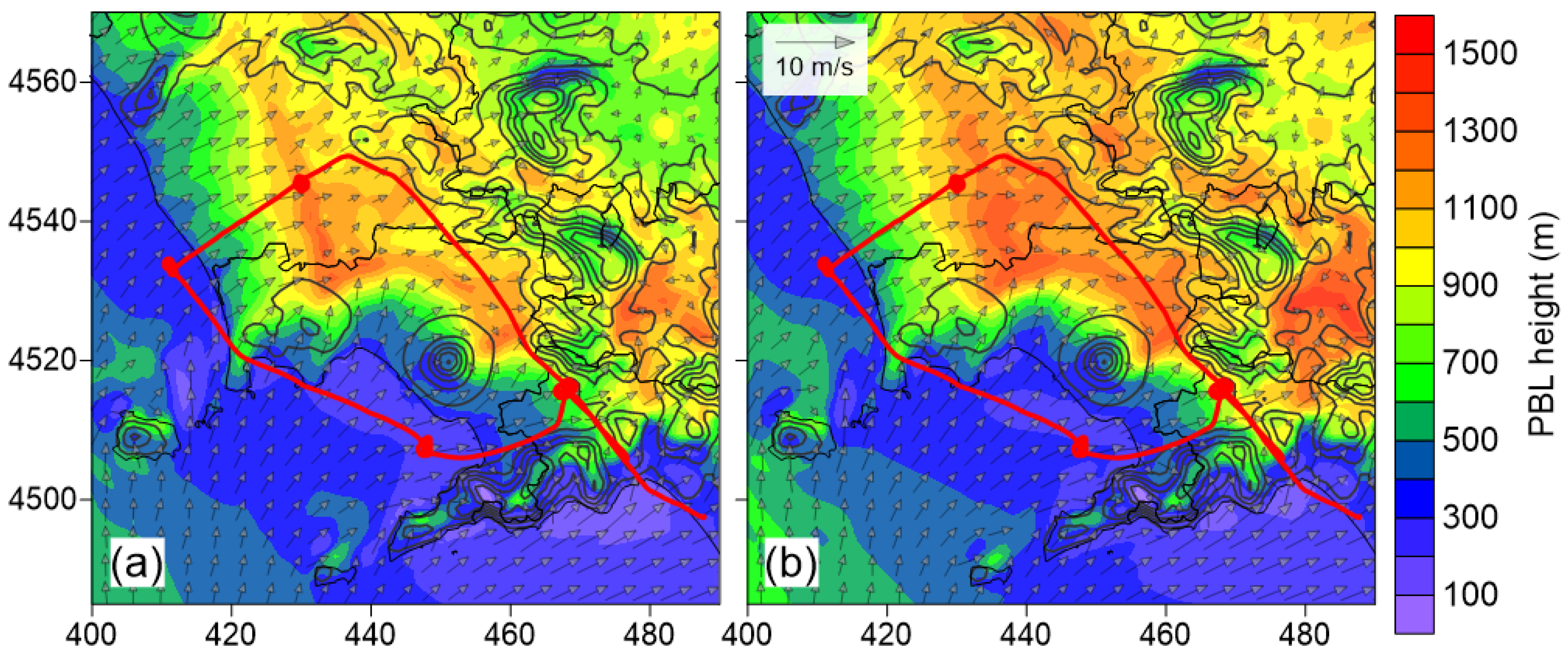
3.4. Comparison of Observed and Modeled PBL Height

The PBL height predicted by the different schemes and available within the WRF standard output is hardly comparable, because different computational methods can produce different estimates of the PBL height, even with the same meteorological input fields. This condition makes it difficult to distinguish differences due to the method to compute PBL height from those due to the meteorological fields produced by WRF with different parameterizations. Therefore, PBL height has been re-computed for each profile by analyzing potential temperature and wind profiles through the application of a criterion based on the bulk Richardson number (Sorensen 1998) [64] as implemented by the WRF post-processor called UPP (https://dtcenter.org/upp/users/index.php), developed by the National Centers for Environmental Prediction (NCEP). This approach produces comparable results, and differences can be attributed to the structure of the meteorological fields in the lower atmospheric layers. Simulated and measured values are compared and presented in Table 4 for all of the profiles. It is observed that no single scheme can be chosen as the best-performing for PBL height simulation in all of the examined conditions.

MYNN2, which performs better in simulating other meteorological variables, is not always the best-performing scheme in predicting PBL height. BouLac, MYJ, YSU, and ACM2 are able to simulate PBL height in equal good proportion considering all of the flights. However, it can be observed from Table 4 that the simulated PBL heights are closer to observations over land compared to sea. At the same time, the vertical grid spacing of the WRF computational mesh should also be kept into account, which grows with height and is roughly 120 m deep at 500 m agl. The model grid spacing intrinsically limits the precision of the PBL height estimation, and should make consider comparable values within the grid spacing range.

The values resumed in Table 4 illustrate the strong space and time variability of the boundary layer depth over the investigated area. The coastal location, the complex terrain, and the non-uniformity of land cover—as the Naples–Caserta conurbation is characterized by mixed urban and agricultural areas—cause the horizontal variation of the boundary layer structure. The dominant breeze circulation regime characterizing fair weather conditions introduces a time variability that is usually characterized by a decrease of the PBL depth over the inland areas when they are reached by the sea breeze front. These features are partially reproduced by the model whose accuracy is limited by it space resolution, together with the PBL parameterization scheme features.

4. Conclusions

WRF model simulations using different PBL schemes have been compared with aircraft observations and analyzed to assess model performance over a complex coastal study area with associated sea breeze circulations. We have presented a comparison of WRF results with observed vertical profiles of air temperature, specific humidity, wind speed, wind direction, and PBL height, and computed statistical scores for each PBL scheme. The overall performance of WRF with all of the selected schemes is assessed on vertical profiles that indirectly indicate the reconstruction of local scale circulation and sea breeze development. The performance criteria for meteorological model results [66,67] were able to distinguish the better-performing PBL schemes out of all of the model runs. As the aircraft observations include high frequency PBL turbulence fluctuations that are filtered out in the WRF model results as a subgrid scale turbulent component of meteorological variables, this reproduction is proving the model’s ability to simulate the conditions on a smaller scale aptly. Overall, the findings of the present study are consistent with Gioli et al. [65], indicating that the sea breeze transition is a critical phenomenon to be correctly simulated in time and space with a WRF-based modeling setup.

No single boundary layer turbulence scheme can be termed as the optimal PBL scheme for all of the tests performed at different times and in different locations within the present study. However, the TKE closure scheme MYNN2 was the best performing in regard to simulating meteorological variables in accordance with normalized cumulated statistical indexes. The results from this study constitute a solid framework that could be followed for the initial performance assessment of a modeling chain, and the identification of the optimal setup for a specific study area. However, aircraft measurements should be also made in different seasons of the year in order to verify the consistency of results. Besides other factors that shall be considered when identifying the PBL scheme to be used in a WRF modeling chain, such as the computational performance, the methodology proposed here can add a level of information to better drive such choice, which is often made arbitrarily. The limitations to all of the PBL schemes and the WRF configuration presented here arise from the model capacity of reproducing sea breeze circulations and the presence of return current layers. The wind speed and direction representation for the lowest 500 m is generally excellent for the better PBL schemes, while the sudden change of wind direction due to the presence of circulation layers is not well reproduced by any of the schemes at all of the locations monitored by vertical profiles, where local differences are detected. Our findings point out that a valid modeling methodology to reduce uncertainties would be running model ensembles of the better-performing PBL schemes and deploying modeling architectures that are commonly used in Earth system sciences [68], although at the cost of a higher demand of computing power.

References

1. Schmale, J.; Schindell, D.; von Schneidemesser, E.; Chabay, I.; Lawrence, M. Air Pollution: Clean up our skies. Nature 2014, 515, 335–337. [Google Scholar] [CrossRef] [PubMed]
2. Zhang, Y.; Sartelet, K.; Wu, S.Y.; Seigneur, C. Application of WRF/Chem-MADRID and WRF/Polyphemus in Europe—Part 1: Model description, evaluation of meteorological predictions, and aerosol-meteorology interactions. Atmos. Chem. Phys. 2013, 13, 6807–6843. [Google Scholar] [CrossRef]
3. Angevine, W.M.; Eddington, L.; Durkee, K.; Fairall, C.; Bianco, L.; Brioude, J. Meteorological Model Evaluation for CalNex 2010. Mon. Weather Rev. 2012, 140, 3885–3906. [Google Scholar] [CrossRef]
4. Kim, Y.; Sartelet, K.; Raut, J.C.; Chazette, P. Evaluation of the Weather Research and Forecast/Urban Model over Greater Paris. Bound.-Layer Meteorol. 2013, 149, 105–132. [Google Scholar] [CrossRef]
5. Govardhan, G.; Nanjundiah, R.S.; Satheesh, S.K.; Krishnamoorthy, K.; Kotamarthi, V.R. Performance of WRF-Chem over Indian region: Comparison with measurements. J. Earth Syst. Sci. 2015, 124, 875–896. [Google Scholar] [CrossRef]
6. Arunachalam, S.; Holland, A.; Do, B.; Abraczinskas, M. A quantitative assessment of the influence of grid resolution on predictions of future year air quality in North Carolina, USA. Atmos. Environ. 2006, 40, 5010–5026. [Google Scholar] [CrossRef]
7. Borge, R.; Alexandrov, V.; del Vas, J.J.; Lumbreras, J.; Rodrıguez, E. A comprehensive sensitivity analysis of the WRF model for air quality applications over the Iberian Peninsula. Atmos. Environ. 2008, 42, 8560–8574. [Google Scholar] [CrossRef] [Green Version]
8. Misenis, C.; Zhang, Y. An examination of sensitivity of WRF/Chem predictions to physical parameterizations, horizontal grid spacing, and nesting options. Atmos. Res. 2010, 97, 315–334. [Google Scholar] [CrossRef]
9. Skamarock, W.C.; Klemp, J.B.; Dudhia, J.; Gill, D.O.; Barker, D.M.; Duda, M.G.; Huang, X.Y.; Wang, W.; Powers, J.G. A Description of the Advanced Research WRF Version 3; National Centre of Atmospheric Research: Boulder, CO, USA, 2008. [Google Scholar]
10. Yver, C.E.; Graven, H.D.; Lucas, D.D.; Cameron-Smith, P.J.; Keeling, R.F.; Weiss, R.F. Evaluating transport in the WRF model along the California coast. Atmos. Chem. Phys. 2013, 13, 1837–1852. [Google Scholar] [CrossRef] [Green Version]
11. Finardi, S.; Agrillo, G.; Baraldi, R.; Calori, G.; Carlucci, P.; Ciccioli, P.; D’Allura, A.; Gasbarra, D.; Gioli, B.; Magliulo, V.; et al. Atmosphericdynamics and ozone cycle during seabreeze in a Mediterranean complex urbanized coastal site. J. Appl. Meteorol. Climatol. 2018, 57, 1083–1099. [Google Scholar] [CrossRef]
12. Silibello, C.; Calori, G.; Brusasca, G.; Giudici, A.; Angelino, E.; Fossati, G.; Peroni, E.; Buganza, E. Modelling of PM10 Concentrations over Milano Urban Area Using Two Aerosol Modules. Environ. Model. Softw. 2008, 23, 333–343. [Google Scholar] [CrossRef]
13. Kukkonen, J.; Olsson, T.; Schultz, M.; Baklanov, A.; Klein, T.; Miranda, I.; Monteiro, A.; Hirtl, M.; Tarvainen, V.; Boy, M.; et al. A review of operational, regional-scale, chemicalweatherforecastingmodels in Europe. Atmos. Chem. Phys. 2012, 12, 1–87. [Google Scholar] [CrossRef] [Green Version]
14. Gioli, B.; Miglietta, F.; Vaccari, F.P.; Zaldei, A.; DeMartino, B. The Sky Arrow ERA, an innovative airborne platform to monitor mass, momentum and energy exchange of ecosystems. Ann. Geophys. 2006, 49, 109–116. [Google Scholar]
15. Zhong, S.; In, H.; Clements, C. Impact of turbulence, land surface, and radiation parameterizations on simulated boundary layer properties in a coastal environment. J. Geophys. Res. 2007, 112. [Google Scholar] [CrossRef] [Green Version]
16. Shin, H.H.; Hong, S.Y. Intercomparison of Planetary Boundary-Layer Parametrizations in the WRF Model for a Single Day from CASES-99. Bound.-Layer Meteorol. 2011, 139, 261–281. [Google Scholar] [CrossRef]
17. Mohan, M.; Bhati, S. Analysis of WRF Model Performance over Subtropical Region of Delhi, India. Adv. Meteorol. 2011, 2011, 621235. [Google Scholar] [CrossRef]
18. Xie, B.; Fung, J.C.H.; Chan, A.; Lau, A. Evaluation of nonlocal and local planetary boundary layer schemes in the WRF model. J. Geophys. Res. 2012, 117, D12103. [Google Scholar] [CrossRef]
19. Madala, S.; Satyanarayana, A.N.V.; Srinivas, C.V.; Kumar, M. Mesoscale atmospheric flow field simulations for air quality modeling over complex terrain region of Ranchi in eastern India using WRF. Atmos. Environ. 2015, 107, 315–328. [Google Scholar] [CrossRef]
20. Madala, S.; Satyanarayana, A.N.V.; Srinivas, C.V.; Tyagi, B. Performance Evaluation of PBL Schemes of WRF-ARW Model in the Simulating Thermo-Dynamical Structure of Pre-monsoon convective Episodes over Kharagpur using STORM Data Sets. Pure Appl. Geophys. 2016, 173, 1803–1827. [Google Scholar] [CrossRef]
21. Banks, R.F.; Tiana-Alsina, J.; Rocadenbosch, F.; Baldasano, J.M. Performance Evaluation of the Boundary-Layer Height from Lidar and the Weather Research and Forecasting Model at an Urban Coastal Site in the North-East Iberian Peninsula. Bound.-Layer Meteorol. 2015, 157, 265–292. [Google Scholar] [CrossRef] [Green Version]
22. Banks, R.F.; Tiana-Alsina, J.; Baldasano, J.M.; Rocadenbosch, F.; Papayannis, A.; Solomos, S.; Tzanis, C.G. Sensitivity of boundary-layer variables to PBL schemes in the WRF model based on surface meteorological observations, lidar, and radiosondes during the HygrA-CD campaign. Atmos. Res. 2016, 176–177, 185–201. [Google Scholar] [CrossRef]
23. Li, X.; Pu, Z. Sensitivity of numerical simulation of early rapid intensification of hurricane Emily (2005) to cloud microphysical and planetary boundary layer parameterizations. Mon. Weather Rev. 2008, 136, 4819–4838. [Google Scholar] [CrossRef]
24. Hu, X.M.; Nielson-Gammon, J.W.; Zhang, F. Evaluation of three Planetary Boundary Layer schemes in the WRF model. J. Appl. Meteorol. Climatol. 2010, 49, 1831–1844. [Google Scholar] [CrossRef]
25. Garcia-Diez, M.; Fernandez, J.; Fita, L.; Yague, C. Seasonal dependence of WRF model biases and sensitivity to PBL schemes over Europe. Q. J. R. Meteorol. Soc. 2013, 139, 501–514. [Google Scholar] [CrossRef]
26. Cohen, A.E.; Cavallo, S.M.; Coniglio, M.C.; Brooks, H.E. A review of planetary boundary layer parameterization schemes and their sensitivity in simulating southeastern U.S. cold season severe weather environments. Weather Forecast. 2015, 30, 591–612. [Google Scholar] [CrossRef]
27. Qian, Y.; Yan, H.; Berg, L.; Hagos, S.; Feng, Z.; Yang, B.; Huang, M. Assessing impacts of PBL and surface layer schemes in simulating the surface-atmosphere interactions and precipitation over the tropical ocean using observations from AMIE/DYNAMO. J. Clim. 2016, 29, 8191–8210. [Google Scholar] [CrossRef]
28. Demographic Balance Data. 2014. Available online: http://demo.istat.it (accessed on 22 June 2018).
29. Martuzzi, M.; Mitis, F.; Bianchi, F.; Minichilli, F.; Comba, P.; Fazzo, L. Cancer mortality and congenital anomalies in a region of Italy with intense environmental pressure due to waste. Occup. Environ. Med. 2009, 66, 725–732. [Google Scholar] [CrossRef] [PubMed] [Green Version]
30. Fazzo, L.; de Santis, M.; Mitis, F.; Benedetti, M.; Martuzzi, M.; Comba, P.; Fusco, M. Ecological studies of cancer incidence in an area interested by dumping waste sites in Campania (Italy). Ann. Ist. Super. Sanita 2011, 47, 181–191. [Google Scholar] [PubMed]
31. Pirastu, R.; Zona, A.; Ancona, C.; Bruno, C.; Fano, V.; Fazzo, L.; Iavarone, I.; Minichilli, F.; Mitis, F.; Pasetto, R.; et al. Mortality results in SENTIERI Project. Epidemiol. Prev. 2011, 35, 29–152. [Google Scholar] [PubMed]
32. Triassi, M.; Alfano, R.; Illario, M.; Nardone, A.; Caporale, O.; Montuori, P. Environmental Pollution from Illegal Waste Disposal and Health Effects: A Review on the “Triangle of Death”. Int. J. Environ. Res. Public Health 2015, 12, 1216–1236. [Google Scholar] [CrossRef] [PubMed] [Green Version]
33. Barone, G.; D’Ambra, P.; di Serafino, D.; Giunta, G.; Murli, A.; Riccio, A. Application of a parallel photochemical air quality model to the Campania region (southern Italy). Environ. Model. Softw. 2000, 15, 503–511. [Google Scholar] [CrossRef]
34. Vellinga, O.S.; Dobosy, R.J.; Dumas, E.J.; Gioli, B.; Elbers, J.A.; Hutjes, R.W.A. Calibration and quality assurance of flux observations from a small research aircraft. J. Atmos. Ocean. Technol. 2013, 30, 161–181. [Google Scholar] [CrossRef]
35. Dobosy, R.; Dumas, E.J.; Senn, D.L.; Baker, B.; Seyres, D.S.; Witinski, M.F.; Healy, C.; Munster, J.; Anderson, J.G. Calibration and quality assurance of an airborne turbulence probe in an aeronautical wind tunnel. J. Atmos. Ocean. Technol. 2013, 30, 182–196. [Google Scholar] [CrossRef]
36. WRF User Manual, 2015 ARW Version 3 Modeling System User’s Guide. January 2015. Available online: http://www2.mmm.ucar.edu/wrf/users/docs/user_guide_V3.5/ARWUsersGuideV3.pdf (accessed on 22 June 2018).
37. Vogelezang, D.H.P.; Holtslag, A.A.M. Evaluation and model impacts of alternative boundary-layer height formulations. Bound.-Layer Meteorol. 1996, 81, 245–269. [Google Scholar] [CrossRef]
38. Pleim, J.E. A combined local and non-local closure model for the atmospheric boundary layer. Part 1: Model description and testing. J. Appl. Meteorol. Climatol. 2007, 46, 1383–1395. [Google Scholar] [CrossRef]
39. Blackadar, A.K. Modeling pollutant transfer during daytime convection. In Preprints Fourth Symposium on Atmospheric Turbulence, Diffusion, and Air Quality; American Meteorological Society: Reno, NV, USA, 1978; pp. 443–447. [Google Scholar]
40. Hong, S.Y.; Pan, H.L. Nonlocal boundary layer vertical diffusion in a medium-range forecast model. Mon. Weather Rev. 1996, 124, 2322–2339. [Google Scholar] [CrossRef]
41. Troen, L.; Mahrt, L. A simple model of the atmospheric boundary layer: Sensitivity to surface evaporation. Bound.-Layer Meteorol. 1986, 37, 129–148. [Google Scholar] [CrossRef]
42. Wyngaard, J.C.; Brost, R.A. Top-down and bottom-up diffusion of a scalar in the convective boundary layer. J. Atmos. Sci. 1984, 41, 102–112. [Google Scholar] [CrossRef]
43. Stull, R.B. Review of non-local mixing in turbulent atmospheres: Transilient turbulence theory. Bound.-Layer Meteorol. 1993, 62, 21–96. [Google Scholar] [CrossRef]
44. Hong, S.Y.; Noh, Y.; Dudhia, J. A new vertical diffusion package with an explicit treatment of entrainment processes. Mon. Weather Rev. 2006, 134, 2318–2341. [Google Scholar] [CrossRef]
45. Lobocki, L. Mellor-Yamada simplified second-order closure models: Analysis and application of the generalized von Karman local similarity hypothesis. Bound.-Layer Meteorol. 1992, 59, 83–109. [Google Scholar] [CrossRef]
46. Janjic, Z. Nonsingular Implementation of the Mellor-Yamada Level 2.5 Scheme in the NCEP Meso Model; NCEP Office Note, No. 437; National Centers for Environmental Prediction: College Park, MD, USA, 2002; p. 61.
47. Janjic, Z. The step-mountain coordinate: Physical package. Mon. Weather Rev. 1990, 118, 1429–1443. [Google Scholar] [CrossRef]
48. Coniglio, M.C.; Correia, J., Jr.; Marsh, P.T.; Kong, F. Verification of convection-allowing WRF model forecasts of the planetary boundary layer using sounding observations. Weather Forecast. 2013, 28, 842–862. [Google Scholar] [CrossRef]
49. Mellor, G.L.; Yamada, T. A hierarchy of turbulence closure models for planetary boundary layers. J. Atmos. Sci. 1974, 31, 1791–1806. [Google Scholar] [CrossRef]
50. Mellor, G.L.; Yamada, T. Development of a turbulence closure model for geophysical fluid problems. Rev. Geophys. Space Phys. 1982, 20, 851–875. [Google Scholar] [CrossRef]
51. Nakanishi, M. Improvement of the Mellor–Yamada turbulence closure model based on large-eddy simulation data. Bound.-Layer Meteorol. 2001, 99, 349–378. [Google Scholar] [CrossRef]
52. Nakanishi, M.; Niino, H. An improved Mellor–Yamada level-3 model with condensation physics: Its design and verification. Bound.-Layer Meteorol. 2004, 112, 1–31. [Google Scholar] [CrossRef]
53. Nakanishi, M.; Niino, H. Development of an improved turbulence closure model for the atmospheric boundary layer. J. Meteorol. Soc. Jpn. 2009, 87, 895–912. [Google Scholar] [CrossRef]
54. Bougeault, P.; Lacarrere, P. Parameterization of orography-induced turbulence in amesobeta-scale model. Mon. Weather Rev. 1989, 117, 1872–1890. [Google Scholar] [CrossRef]
55. Martilli, A.; Clappier, A.; Rotach, M.W. An urban surface exchange parameterisation for mesoscale models. Bound.-Layer Meteorol. 2002, 104, 261–304. [Google Scholar] [CrossRef]
56. Grenier, H.; Bretherton, C.S. A moist PBL parameterization for large-scale models and its application to subtropical cloud-topped marine boundary layers. Mon. Weather Rev. 2001, 129, 357–377. [Google Scholar] [CrossRef]
57. Bretherton, C.; Park, S. A new moist turbulence parameterization in the community atmosphere model. J. Clim. 2009, 22, 3422–3448. [Google Scholar] [CrossRef]
58. Gent, P.R.; Danabasoglu, G.; Donner, L.J.; Holland, M.M.; Hunke, E.C.; Jayne, S.R.; Lawrence, D.M.; Neale, R.B.; Rasch, P.J.; Vertenstein, M.; et al. The Community Climate System Model Version 4. J. Clim. 2011, 24, 4973–4991. [Google Scholar] [CrossRef] [Green Version]
59. Wyngaard, J.C. Toward Numerical Modeling in the “Terra Incognita”. J. Atmos. Sci. 2004, 61, 1816–1826. [Google Scholar] [CrossRef]
60. Ito, J.; Niino, H.; Nakanishi, M.; Moeng, C. An Extension of the Mellor–Yamada Model to the TerraIncognita Zone for Dry Convective Mixed Layersin the Free Convection Regime. Bound.-Layer Meteorol. 2015, 157, 23–43. [Google Scholar] [CrossRef]
61. Skamarock, W.C. Evaluating Mesoscale NWP Models Using Kinetic Energy Spectra. Mon. Weather Rev. 2004, 132, 3019–3032. [Google Scholar] [CrossRef]
62. Wang, X.Y.; Wang, K.C. Estimation of atmospheric mixing layer height from radiosonde data. Atmos. Meas. Tech. 2014, 7, 1701–1709. [Google Scholar] [CrossRef] [Green Version]
63. Seidel, D.J.; Ao, C.O.; Li, K. Estimating climatological planetary boundary layer heights from radiosonde observations: Comparison of methods and uncertainty analysis. J. Geophys. Res. 2010, 115. [Google Scholar] [CrossRef] [Green Version]
64. Sorensen, J.H. Sensitivity of the DERMA long-range Gaussian dispersion model to meteorological input and diffusion parameters. Atmos. Environ. 1998, 32, 4195–4206. [Google Scholar] [CrossRef]
65. Gioli, B.; Gualtieri, G.; Busillo, C.; Calastrini, F.; Gozzini, B.; Miglietta, F. Aircraft wind measurements to assess a coupled WRF-CALMET mesoscale system. Meteorol. Appl. 2014, 21, 117–128. [Google Scholar] [CrossRef]
66. Thunis, P.; Georgieva, E.; Galmarini, S. A Procedure for Air Quality Models Benchmarking, FAIRMODE Report Version 2. 2011. Available online: http://fairmode.jrc.ec.europa.eu/ (accessed on 22 June 2018).
67. Enhanced Meteorological Modeling and Performance Evaluation for Two Texas Ozone Episodes. Available online: https://www.tceq.texas.gov/assets/public/implementation/air/am/contracts/reports/mm/EnhancedMetModelingAndPerformanceEvaluation.pdf (accessed on 22 June 2018).
68. Yuan, X.; Wood, E.F. On the clustering of climate models in ensemble seasonal forecasting. Geophys. Res. Lett. 2012, 39. [Google Scholar] [CrossRef] [Green Version]
Figure 1. Flight tracks performed by the Sky Arrow aircraft on 8 October 2014 (sky blue color lines). Locations of four profiles (PRF), i.e., P1 (40°47′39.35″ N, 14°37′52.82″ E), P2 (40°57′05.68″ N, 13°56′19.41″ E), P3 (40°45′12.89″ N, 14°18′00.54″ E), and P4 (41°04′22.49″ N, 14°10′06.27″ E) are outlined by yellow circles (image source: Google Earth).
Atmosphere 09 00272 g001
Figure 2. Geographic location of Weather Research and Forecasting (WRF) four nested domains (a) and a zoom over the two inner ones, covering the Campania Region and Naples (b). Image source: Google Earth.
Atmosphere 09 00272 g002
Figure 3. Surface pressure charts showing pressure and weather fronts at 00:00 UTC of 8–10 October 2014 (left panel ac). Charts are provided by the Met Office and available at http://www.wetterzentrale.de. Thickness isopleths for the layer (500–1000) hPa (dam) and temperature at 850 hPa (°C) at 00:00 UTC of 8, 9 and 10 October 2014 (right panel a1c1). Charts are provided by ECMWF reanalysis (ERA-Interim) and available at http://www.meteociel.fr.
Atmosphere 09 00272 g003aAtmosphere 09 00272 g003b
Figure 4. Napoli Capodichino airport (LIRN) surface meteorological observations (blue) and WRF simulation results with the Mellor–Yamada–Nakanishi–Niino Level 2.5 (MYNN2)planetary boundary layer (PBL) scheme (red) for: (a) pressure; (b) wind speed and direction; (c) air temperature; and (d) relative humidity.
Atmosphere 09 00272 g004
Figure 5. Vertical profile of (a) air temperature (°C); (b) wind speed (m/s); (c) specific humidity (g/kg); and (d) wind direction (degree) on 8 October 2014 during Flight 3: Profile 1 up. Error bars in observations are standard deviation values.
Atmosphere 09 00272 g005
Figure 6. Vertical profile of (a) air temperature (°C); (b) wind speed (m/s); (c) specific humidity (g/kg); and (d) wind direction (degree) on 8 October 2014 during Flight 3: Profile 2 up. Error bars in observations are standard deviation values.
Atmosphere 09 00272 g006
Figure 7. Vertical profile of (a) air temperature (°C); (b) wind speed (m/s); (c) specific humidity (g/kg); and (d) wind direction (degree) on 8 October 2014 during Flight 3: Profile 3 up. Error bars in observations are standard deviation values.
Atmosphere 09 00272 g007
Figure 8. Vertical profile of (a) air temperature (°C); (b) wind speed (m/s); (c) specific humidity (g/kg); and (d) wind direction (degree) on 8 October 2014 during Flight 3: Profile 4 up. Error bars in observations are standard deviation values.
Atmosphere 09 00272 g008
Figure 9. PBL height (m) predicted by WRF model simulations for 8 October 2014 at 13:00 GMT with MYNN2 (panel a) and Yonsei University (YSU) (panel b) PBL parameterization. Wind field at 10-m height is represented by grey arrows (one arrow out of four). The red line superposed represents the flight track.
Atmosphere 09 00272 g009
Figure 10. Variation of Pearson coefficient for PBL schemes used in the present study for all of the flights (flights 1–5) for air temperature, specific humidity, wind direction, and wind speed for morning/afternoon (a,c,e,g) and over sea/inland (b,d,f,h) respectively.
Atmosphere 09 00272 g010
Figure 11. Variation of root mean square error (RMSE) for PBL schemes used in the present study for all flights (flights 1–5) for air temperature, specific humidity, wind direction, and wind speed for morning/afternoon (a,c,e,g) and over sea/inland (b,d,f,h) respectively.
Atmosphere 09 00272 g011
Figure 12. Variation of normalized RMSE (a) and normalized correlation (b) for PBL schemes used in the present study for all of the meteorological variables and profiles.
Atmosphere 09 00272 g012