The Three-Dimensional Locating of VHF Broadband Lightning Interferometers


1
Laboratory of Lightning Physics and Protection Engineering, State Key Laboratory of Severe Weather, Chinese Academy of Meteorological Sciences, Beijing 100081, China
2
National Key Laboratory on Electromagnetic Environmental Effects and Electro-Optical Engineering, Army Engineering University, Nanjing 210007, China
*
Authors to whom correspondence should be addressed.
Atmosphere 2018, 9(8), 317; https://doi.org/10.3390/atmos9080317
Submission received: 23 June 2018
/
Revised: 27 July 2018
/
Accepted: 10 August 2018
/
Published: 13 August 2018
(This article belongs to the Section Meteorology)
Abstract
:VHF (Very High Frequency) lightning interferometers can locate and observe lightning discharges with a high time resolution. Especially the appearance of continuous interferometers makes the 2-D location of interferometers further improve in time resolution and completeness. However, there is uncertainty in the conclusion obtained by simply analyzing the 2-D locating information. Without the support of other 3-D total lightning locating networks, the 2-station interferometer becomes an option to obtain 3-D information. This paper introduces a 3-D lightning location method of a 2-station broadband interferometer, which uses the theodolite wind measurement method for reference, and gives the simulation results of the location accuracy. Finally, using the multi-baseline continuous 2-D locating method and the 3-D locating method, the locating results of one intra-cloud flash and the statistical results of the initiation heights of 61 cloud-to-ground flashes and 80 intra-cloud flashes are given. The results show that the two-station interferometer has high observation accuracy on both sides of the connection between the two sites. The locating accuracy will deteriorate as the distance between the radiation source and the two stations increases or the height decreases. The actual locating results are similar to those of the existing VHF TDOA (Time Difference of Arrival) lightning locating network.
1. Introduction
Lightning detection technology has always played an important role in lightning research [1,2,3]. With the development of microelectronics and optoelectronic technology, lightning detection methods have been improved significantly since the 1970s [4,5,6,7,8,9,10,11,12,13,14,15]. Therefore, people have made breakthrough progress in understanding the distribution structure of positive and negative charge layers in thunderstorms and the discharge processes of intra-cloud flash (IC) and cloud-to-ground flash (CG) at various stages, making it possible to conduct fine research on the lightning development process [16,17,18,19,20,21,22,23]. Among these technologies, VHF (Very High Frequency) lightning detection equipment has become an important technical means to study the initiation mechanism, morphological characteristics, and development of lightning, because it has the ability to observe the lightning breakdown process and is not affected by cloud cover [24,25,26,27].
According to different locating methods, VHF lightning locating systems can be divided into two types: lightning locating networks using Time Difference of Arrival (TDOA) method and VHF lightning interferometer systems using interferometric direction finding method. Compared with TDOA locating system, the lightning interferometer can not only locate isolated pulse signals but continuous emissions as well [28], and the time resolution of the locating result can reach or exceed microsecond level, which is much higher than that of the existing TDOA locating system [29]. Although these advantages can only be fully demonstrated when the interferometer is used for azimuth-elevation 2-D direction finding, the high time resolution 2-D locating of the interferometer can be used for networking observation or in combination with another set of lightning locating system to give full play to its characteristics and describe the lightning discharge process in detail [23,30,31]. Currently, the existing lightning interferometers can be roughly divided into two types: narrow-band interferometers and wide-band interferometers, depending on the bandwidth of the received signals [6,32]. The observed performance of the two types of equipment is similar, but the broadband interferometer can record the VHF broadband radiation waveform of lightning, and can use various digital signal processing methods to optimize the locating results afterward [29,33]. Especially the continuous interferometer using high-speed Analog to Digital (A/D) data acquisition card at present has a high time resolution, a large dynamic range of signal amplitude resolution and continuous sampling recording ability, making the new interferometer able to describe the lightning discharge processes more completely [29].
A single-station broadband interferometer system can only give the locating results of the radiation sources in two dimensions, with which many conclusions can be made based on the estimation. Even if the 3-D information can be estimated by combining the information provided by other synchronous observation systems [22,30,31], there is still an inconvenience and uncertainty in the study of the physical mechanism of discharge. How to use multi-station synchronous 3-D observation to give full play to the advantages of interferometer system is always a problem faced in interferometer observation, and many attempts have been made continuously to overcome this [34,35,36]. This paper introduces a 3-D locating method of a two-station broadband interferometer system and gives the corresponding error analysis and observation results.
2. Equipment and Method
The broadband interferometer system used here has been introduced in the previous work [30,33]. Each broadband interferometer system consists of four parts: the VHF broadband signal acquisition, ground electric field change signal acquisition, and the GPS (Global Positioning System) receiver and controller. Lightning VHF signals acquired by four wideband omnidirectional antennas are converted into digital signals with a sampling rate of 1 GHz and a vertical accuracy of 8 bits by a Leroy 7100 high-speed digital oscilloscope. The bandwidth of VHF observation is about 30~300 MHz. The electric field change meter is used to measure the ground electric field change caused by lightning. The system uses a 12 bits A/D acquisition card to record electric field change signals at a sampling rate of 1 MHz. The GPS receiver provides an external clock and time service for the system. The root mean square error of time service can be better than 50 ns. The computer, as a controller, realizes the control of the oscilloscope and the synchronous acquisition and transmission of VHF signals and ground electric field change signals through RJ45 network ports and provides time information and precise triggering time for the system in combination with the GPS receiver.
The two-station 3-D observation experiment based on this system started in 2007 at the earliest and was conducted again in 2010 after adjustments. The observations in this article were made in the summer of 2010 (from 21 May to 21 July). Two observation sites were located in the Conghua District, Guangdong Province, China. Two sets of broadband interferometer stations were respectively set up at the Meteorological Bureau observation site (Site A, 23.568° N, 113.615° E) and the artificial lightning test field (Site B, 23.639° N, 113.595° E). The altitudes of observation sites A and B were 37 m and 74 m respectively, and the linear distance was about 8.15 km. Square VHF wideband antenna arrays were used for both sites, with baseline lengths of 16 m and 15 m, respectively.
Compared with our previous work, the 2-D locating method used here has been adjusted to some extent. In the previous work, the locating program used a 1024 ns long time window to extract the phase difference spectrum from the three channels of VHF signals with orthogonal baselines. Depending on the analysis object, this window was used to extract signals that reach a certain amplitude threshold or to continuously extract signals at 512 ns intervals in a sliding way. After the calculated phase difference spectrum was unwrapped, the angle of incidence was calculated by using the phase difference of each frequency point in the stronger frequency band of the signal, and was given as the calculation result after averaging. Similar practices are often used in existing similar systems [32,36,37,38]. In recent years, with the appearance of continuous interferometers, the 2-D locating method has also changed. The method of obtaining the time difference between signals by cross-correlation time delay estimation has begun to replace the phase difference calculation that needs to be processed by ambiguity resolution, and the combination of multiple baselines can be used to solve the overdetermined equations to calculate the azimuth and elevation angles of the radiation source [29]. Here, we also introduce the least square method using a multi-baseline combination [39].
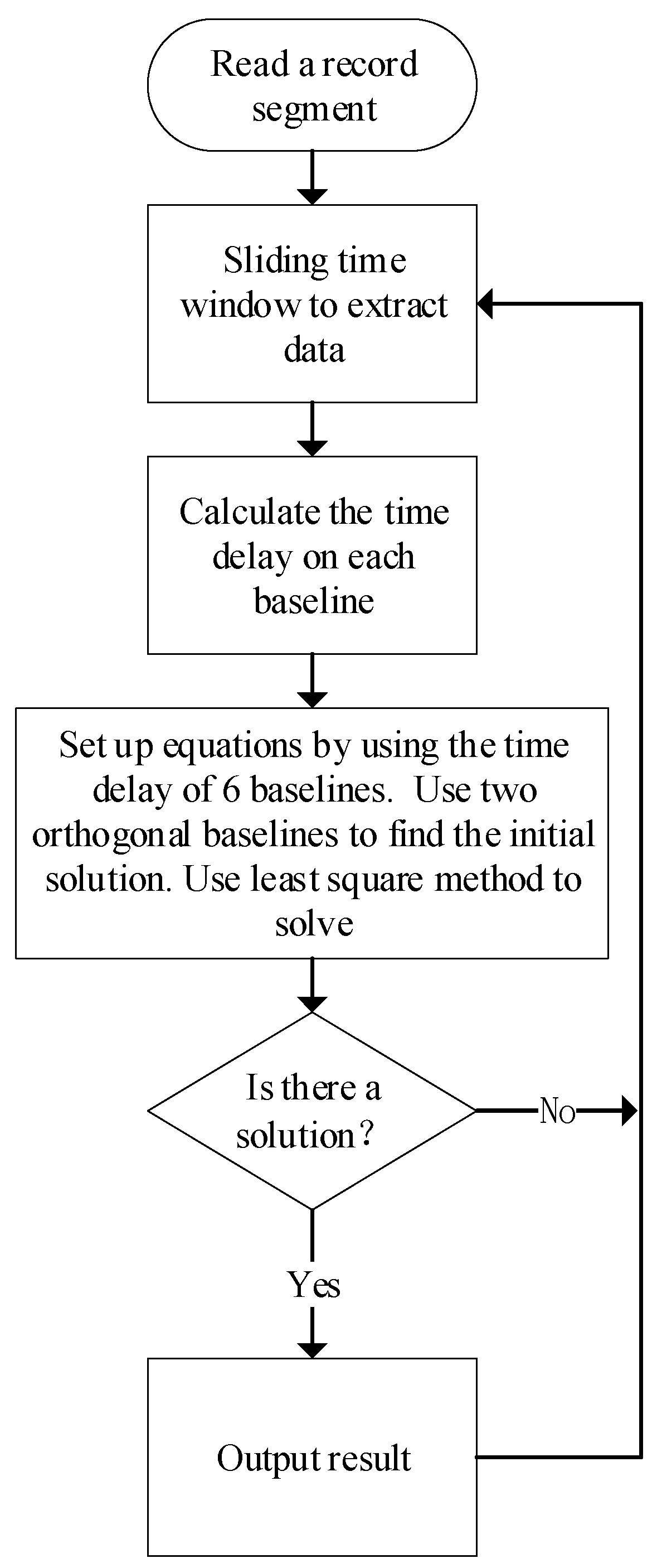
Figure 1 shows the 2-D locating flow used here. Firstly, a segment is read from the data, which consists of signals from four synchronous acquisition channels. The following example uses a segment length of 2048 sample points, i.e., about 2 μs. Subsequently, we used a 1024 ns time window to extract the data, slid at 64 ns intervals. In the third step, the generalized cross-correlation method is used to estimate the time delay of the four channels extracted each time according to the six baseline combinations, and the time difference Δtn between the signals received by the two antennas at each baseline is calculated. Here, n is used to represent the baseline number. For the nth baseline, Δtn and the incidence angle θn satisfy Equation (1), where dn is the length of baseline n and c is the speed of light. The fourth step uses the time difference calculation results of the six baselines to establish equations set up according to Equation (2), wherein α and β are the angles between the incident direction of electromagnetic waves and the north and east directions respectively, and δn is the angle between the nth baseline and the north direction. The least square method is used to solve the equations. Using the existing due north and east baselines in the antenna array, the angle α0 and β0 between the incident signal and the due north and east directions can be directly calculated using Equation (1) and brought into the least square calculation as initial values. Finally, if the equations have solutions and β is not equal to 90° then the obtained α and β are brought into Equations (3) and (4) to find the azimuth AZ and elevation EL of the incident. If β equals 90°, when α is less than 90°, elevation EL equals α, azimuth AZ equals 90°, when α is greater than 90°, elevation EL equals 180° − α, and azimuth AZ equals 270°. After the result is saved, the next calculation will continue until the data of a lightning bolt is completely calculated.
Two groups of the time series corresponding to azimuth and elevation angles can be obtained by solving the arrival directions of the synchronous data collected by the two observation stations respectively. Then 2-D locations of the same target observed by the two sites can be used for 3-D locating. The 3-D solution here is exactly similar to the double theodolite wind measurement in high altitude weather detection [40]. That is, the coordinates of the two sites A and B have been determined, and a set of azimuth and elevation angles relative to the sites have been calculated respectively, so as to solve the 3-D coordinates of the target and reduce the locating error as much as possible. Therefore, we draw lessons from the double theodolite measurement algorithm to solve the 3-D coordinates of the radiation source. The algorithm is shown in Appendix A.
For the geographical environment of each site and the distance between the site and lightning radiation source are different, the radiation sources obtained by each site cannot correspond to each other one by one. Similar to the existing multi-station lightning location, determining whether the observed results at each site come from the same radiation source is a very important step in the 3-D lightning location process of a two-station broadband interferometer observation. This requires designing a reasonable radiation point matching algorithm to find the radiation sources in each site that can correspond to each other, and then solving the 3-D coordinates of the radiation sources through the locating algorithm.
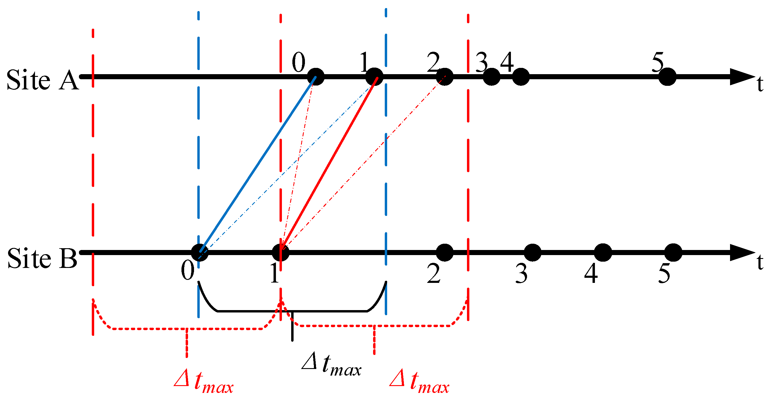
We determine whether the 2-D location results come from the same radiation source by comparing the time-space relationship between the 2-D location results. The program selects a 2-D locating result of one site, and searches for results that meet the time and space conditions among all the 2-D locating results of another site. The time condition means that, as the observation records the same radiation source at two stations, the time difference between the triggering times of the two records cannot be greater than the time difference caused by the electromagnetic wave incident along the connecting line between the two stations. If the two stations are 8.15 km apart, the maximum time difference allowed by the two-site layout is about 27.2 μs. As shown in Figure 2, t is the time axis, and each black dot on it represents the time of the radiation point obtained by each site. To find the corresponding point at site A, site B first selects the point with the serial number 0, and then searches for possible matching points in the data of site A according to the maximum time difference Δtmax allowed by the distance between two sites. Δtmax is equal to the time it takes for light to travel between two sites. As shown in Figure 2, the time range is bounded by the two blue dashed lines. With this as the limiting condition, there is the possibility of corresponding multiple radiation points at site A for one radiation point observed from site B. The time condition can greatly reduce the range of 2-D locating results that may meet the requirements.
If there are multiple combinations of a radiation source that meet the matching conditions, we will use the 3-D location calculation method in Appendix A to calculate the 3-D locations determined by the selected 2-D locating result of site B and all the 2-D locating results of site A that meet the time conditions. Under ideal conditions, the space condition should be set to the same radiation source and the directional rays observed by the two observation stations should be able to converge at one point. However, due to errors in actual observation, the two directional rays are mostly in different planes. Therefore, the combination with the smallest length of the common vertical line segment between the directional rays should be selected as a pair of 2-D locating results from the same radiation source. If both points 0 and 1 of site A meet the requirements, the spatial positions of the radiation sources of the two combinations are calculated respectively, and the combination 0-0 with the smallest common vertical line segment R3 (Equation (A6)) is selected as the best match. According to this method, the matching points 0, 1, and 2 at site A can be obtained respectively by carrying out similar processing on point 1 at site B. Unlike the first point 0, when the subsequent point of site B uses the maximum time difference Δtmax to select possible matching points, it will outline the time window in two directions of the time axis as shown by the three red dashed lines in Figure 2. Then the program selects the combination of 1-1 with the smallest R3 as the best match. Here, the connection between two points in each of 0-0 and 1-1 is only a schematic diagram and does not represent the length of R3. The spatial condition here is a hypothesis to determine the solution. The result that meets the condition is a possible optimal solution and not necessarily a real solution.
After obtaining the 3-D location, we will know the relative position between the radiation source and the two observation stations. Then, the correctness of the matching is judged according to the time difference between the arrivals of electromagnetic waves at the two observation sites from the location of the radiation source. We will check whether the relative position between the locating result and the two stations is inconsistent with the actually observed arrival time, that is, the stations close to the radiation source should receive the electromagnetic waves of the radiation source first.
According to the oscilloscope’s technical manual, the interval between the two adjacent trigger segments in the oscilloscope segmented recording mode is about 6 μs. In most cases, this time interval is about 2~4 μs. This dead time will affect the accuracy of the locating. Affected by the dead time, radiation sources separated by one or more dead times may be matched and used to calculate the 3-D location. Assuming that the discharge development speed is on the order of 107 m/s, the space distance between the two radiation sources separated by one dead time interval is on the order of tens of meters. This error will continue to grow larger if the discharge develops faster or if there are more dead time intervals. Therefore, the use of this 3-D locating method has certain limitations. In actual use, if we use this mode to observe the spatial position and development trend of a lightning flash, then the error of this method is generally acceptable. If we need to study the discharge events with smaller spatial scales, we often use the 3-D locating results as a reference, analyze the 2-D locating results of the two stations in detail, or use the segment mode with a longer segment length to observe the specific lightning discharge events.
3. Locating Accuracy and Error Analysis
The locating error of the two sites is mainly composed of the angle measurement error of each baseline in each site. The angle measurement error of each baseline depends on the phase measurement error, baseline length, signal frequency, and angle of incidence. After the equipment is fixed, the angle measurement error is only related to the angle of incidence. Thus, for any point in the 3-D space, the angle measurement error of each baseline can be obtained according to Equation (5) from the angle of incidence. In the equation, σϕ indicates the phase measurement error, which is generally related to the factors of hardware processing error and system parameter setting. For example, the receiving antenna, coaxial cable, filter, and data acquisition system will all affect the measurement accuracy. d is the baseline length; f is the frequency used for locating; θ indicates the angle between the incident plane wave and the baseline, wherein the phase error σϕ can also be converted into a time error σt. From Equation (5), it can be seen that the system error is the smallest when the signal incident direction is perpendicular to the baseline. In addition, the interaction between antennas and the reflection of signals will also cause fixed system errors, but they will not be considered in the following simulations.
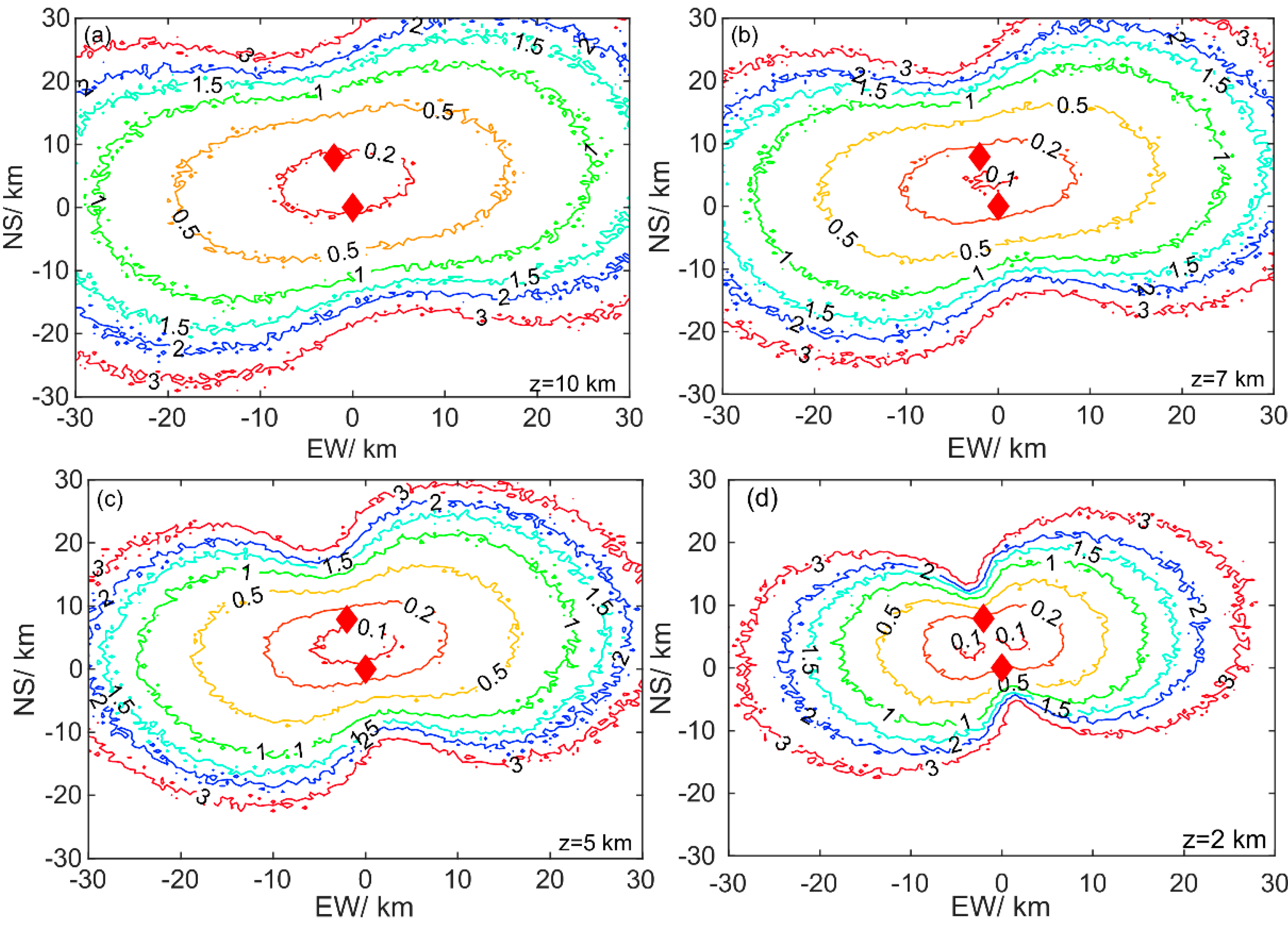
The angle measurement error is superposed with the real incident angle of the simulated radiation source and substituted into the locating algorithm to obtain the 3-D locating point coordinates with errors, and then the locating error at each point in space can be obtained by comparing them with the real coordinates of the radiation source. Using 1 ns as the time delay estimation error and substituting it into Equation (5), the maximum error of the incidence angle is calculated. Site A is taken as the origin of coordinates, the north is the Y-axis, and the east is the X-axis. Using the Monte Carlo method, the locating errors of radiation sources at 10, 7, 5, and 2 km heights are calculated respectively and are given in Figure 3. The errors of the incident angle of the two stations are normally distributed and randomly generated in the simulation. As can be seen from Figure 3, the locating accuracy deteriorates with the increasing distance from the center. For example, at a height of 10 km, the locating accuracy is basically 500 m within 10 km around the center of two sites, most areas within 20 km have a locating accuracy of 1.5 km, and the locating accuracy of areas above 30 km begin to drop to above 2 km. The line of equal precision is peanut-shaped. The range of equal precision in the east-west direction is larger than that in the north-south direction, that is, the system has a better detection capability for the direction perpendicular to the double-station connection line, while the locating accuracy in the direction of the double-station connection line drops fastest. As shown in Figure 3c, the region with the best-locating accuracy appears at a height of 5 km. As the altitude decreases or increases from 5 km, the locating accuracy becomes worse. This result is related to the distance between the two stations.
4. Observation
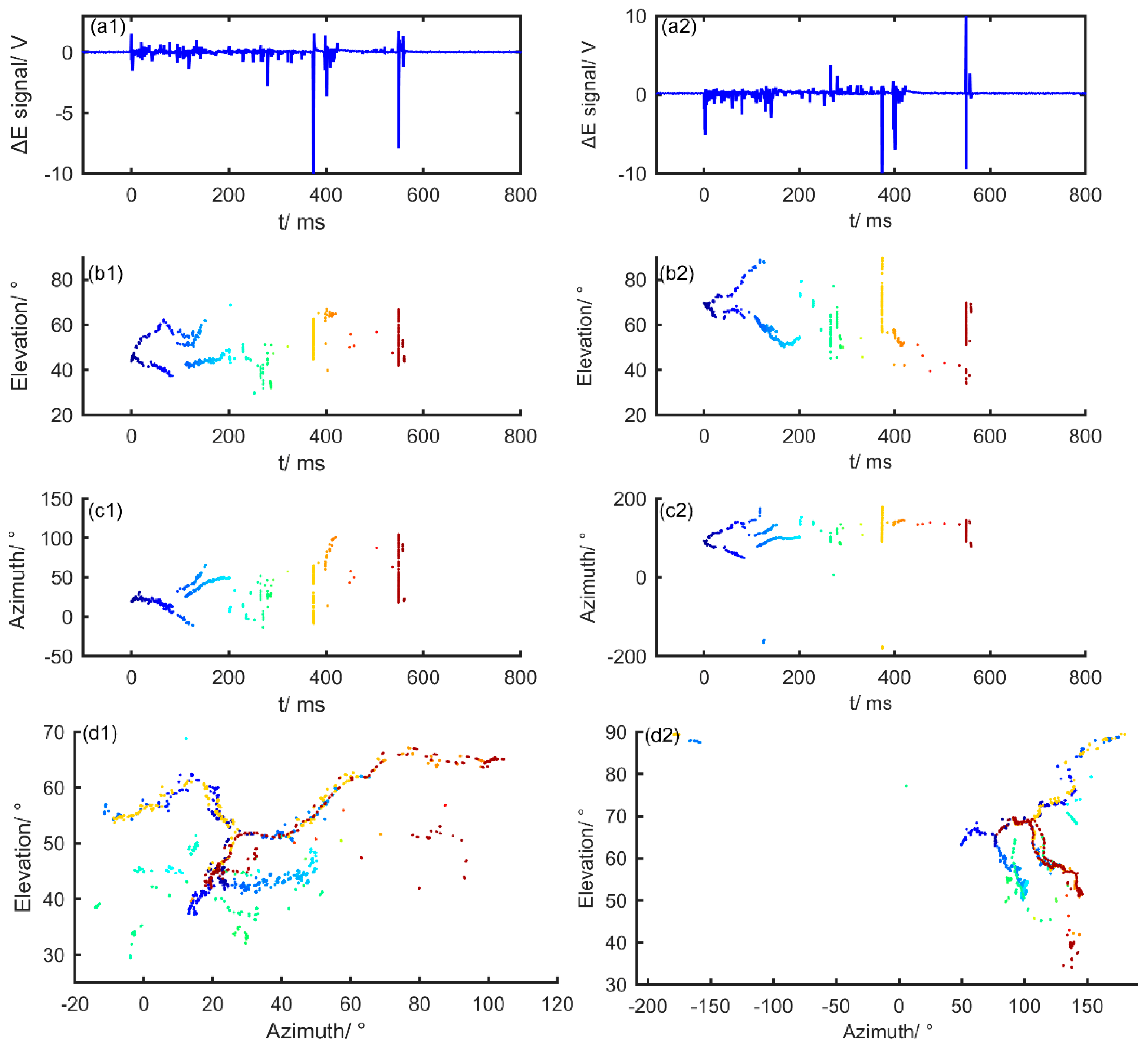
Figure 4 shows the two-station synchronous 2-D locating result of an IC flash occurred at 15:26:17 on 21 July 2010 Beijing time. Wherein (a1), (b1), (c1), and (d1) respectively give the fast electric field change waveform, elevation angle change with time, azimuth angle change with time and azimuth versus elevation 2-D images observed by site A. Correspondingly, the observation results of site B are given by (a2), (b2), (c2), and (d2). In the figure, the electric field change signal is uncalibrated and given in voltage units, and the polarity is defined by physics sign convention, that is, the negative return stroke corresponds to the negative electric field change. The color marks the time when the radiation source occurred. The azimuth angle is 0° in the north direction, counterclockwise to −180°, and clockwise to 180°. VHF radiation from this IC flash was collected by using a segmented trigger method, with each segment length of about 2 μs. The duration of the lightning was about 600 ms. Site A recorded 652 segments of VHF data and 8182 locating points were calculated. Site B recorded 593 segments of data and 6998 locating points were calculated.
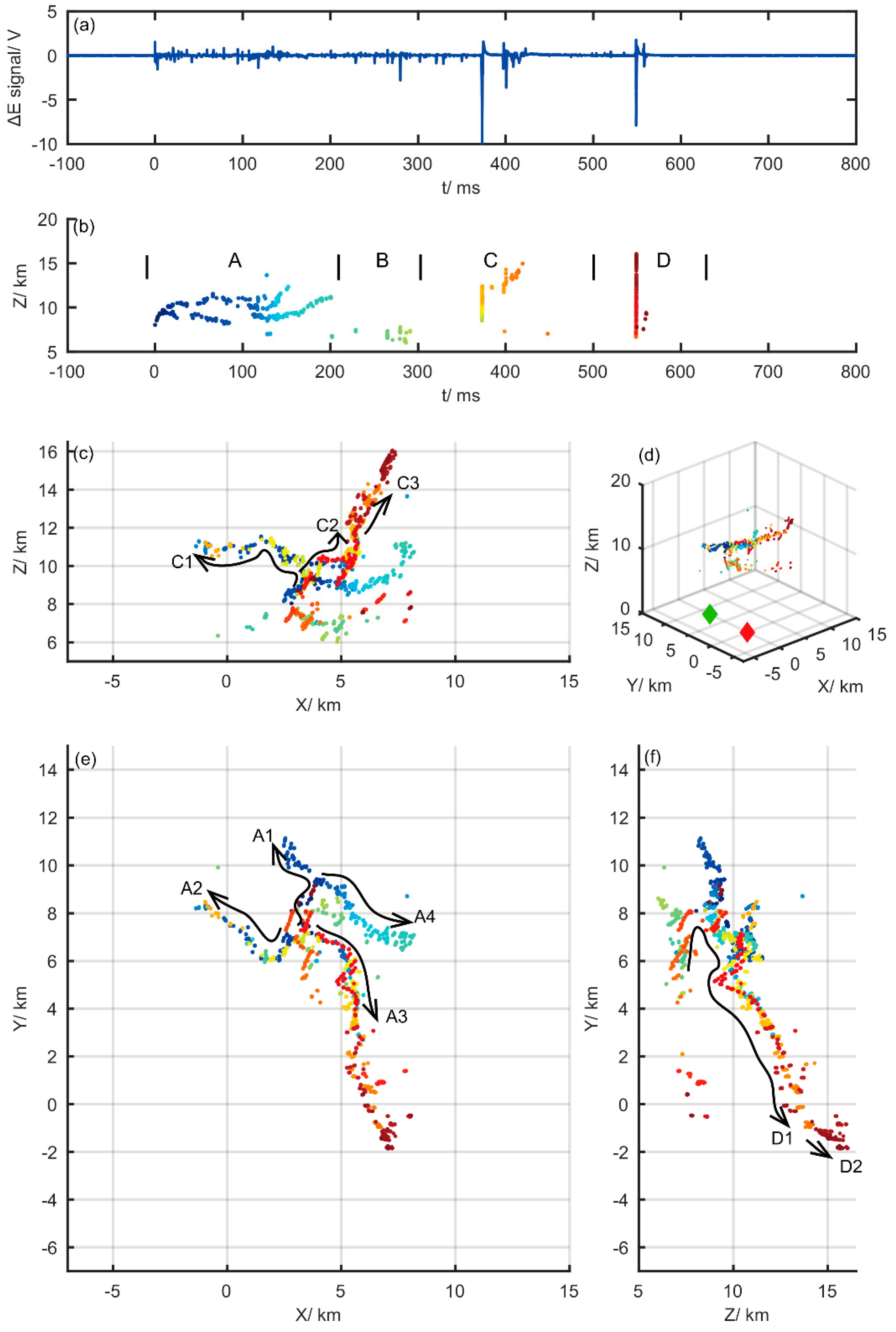
After the two sets of data are brought into the 3-D locating program, the 3-D locating result shown in Figure 5 is obtained. In Figure 5, (a) is the fast electric field change waveform obtained by site A, (b) is the change of the radiation source height with time, (c) is the projection of the 3-D locating result on the X-Z plane, (d) is the 3-D locating result and the two observation sites, (e) is the projection on the X-Y plane, and (f) is the projection on the Y-Z plane. In the figure, the Y-axis direction is the connecting line direction between site A and site B, where site A is located at the origin and site B is located at 8.15 km of the Y-axis positive half shaft. As can be seen from Figure 5d, this lightning bolt occurred in an area with high locating accuracy within 10 km on one side of the connection line between the two sites. This IC flash started at an altitude of 8.4 km. The distribution of the radiation source height shows an obviously layered structure. As shown in Figure 5b, the duration of this IC flash record is about 600 ms. For the convenience of description, this lightning is divided into four periods of time A, B, C, and D.
During period A, the VHF radiation source are first developed simultaneously along the A1 and A2 paths depicted by the arrow curve in Figure 5e. Path 1 stopped after lasting for about 82 ms, with an average development speed of about 5.3 × 10⁴ m/s. Path 2 lasted about 116 ms with an average development speed of about 1.5 × 10⁴ m/s. When path 2 was nearing a stop, the new discharge process began to develop along both paths 3 and 4 from the vicinity of the lightning start position and the middle portion of path 1. Path 3 lasted about 58 ms with an average speed of 8.4 × 10⁴ m/s. Path 4 lasted about 63 ms with an average speed of 7.0 × 10⁴ m/s.
As shown in Figure 5b, most of the lightning VHF radiation sources appeared sporadically below the lightning starting area and were scattered in several directions below the initiation position during the B period. On the whole, these discharge events tended to converge toward the lightning initiation region, which was consistent with the scene of the recoil breakdown process [17].
In Figure 5c, the development path of the 3-D locating result of the lightning VHF radiation source in period C is marked with curved arrows. According to the development path, it can be divided into two stages. In the first stage, the discharges in the C1 and C2 paths developed along the branch paths A2 and A3 of the A period, started below the lightning initiation position, about 0.5 km away from the initiation point, and lasted about 800 μs. The radiation source in this stage first developed upward for a period of time, then developed along the C1 and C2 directions respectively, with average velocities of 9.5 × 10⁶ m/s and 1.7 × 10⁷ m/s. About 100 μs after C2 ended, the discharge of C3 path continued to expand outward at the end of the A3 path, with a duration of about 41 ms and an average speed of about 1.0 × 10⁵ m/s.
Figure 5f shows a rapid breakdown process in the D period with arrows. Similar to the discharge in the C period, it can also be divided into two stages according to the development path. First, D1 started from below the lightning and developed toward the lightning starting position. Then it continued along the previous C2 and C3 paths, with an average development speed of about 3.1 × 10⁷ m/s. After reaching the end of the C3 path, the discharge process continued to expand outward along the D2 path, with an average speed of 4.1 × 10⁷ m/s. At this point, the lightning location record was over.
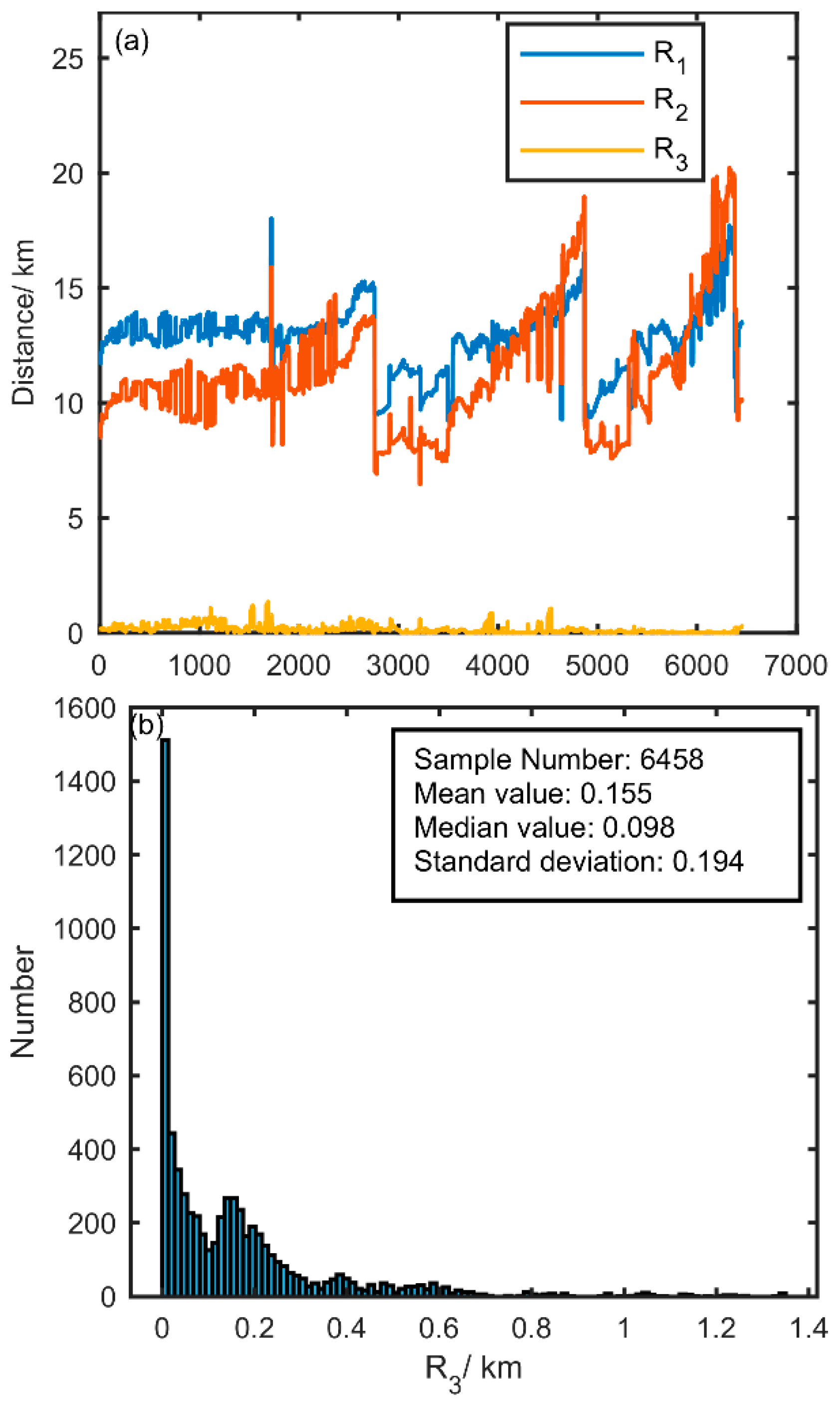
While outputting the 3-D locating result, Figure 6 shows R1, R2, and R3 (Equation (A6)) obtained in the process of calculating the locating result. As shown in Figure 6a, R1 and R2 corresponding to this IC flash location result are approximately equal and much larger than R3, i.e., the distance between the lightning and the two sites is approximately equal and there is no abnormality in the location calculation. As pointed out earlier, R3 can be used to evaluate the error of the 3-D locating result. Figure 6b shows the statistical results of R3 corresponding to all the locating results. It can be seen that the arithmetic mean value of R3 corresponding to the 6458 3-D locating results of this IC flash is 155 m, the standard deviation is 194 m, and the median value is 98 m. There is no limit to the reasonable range of R3 values. In actual use, the range of R3 values can be limited as appropriate to control the quality of the locating results.
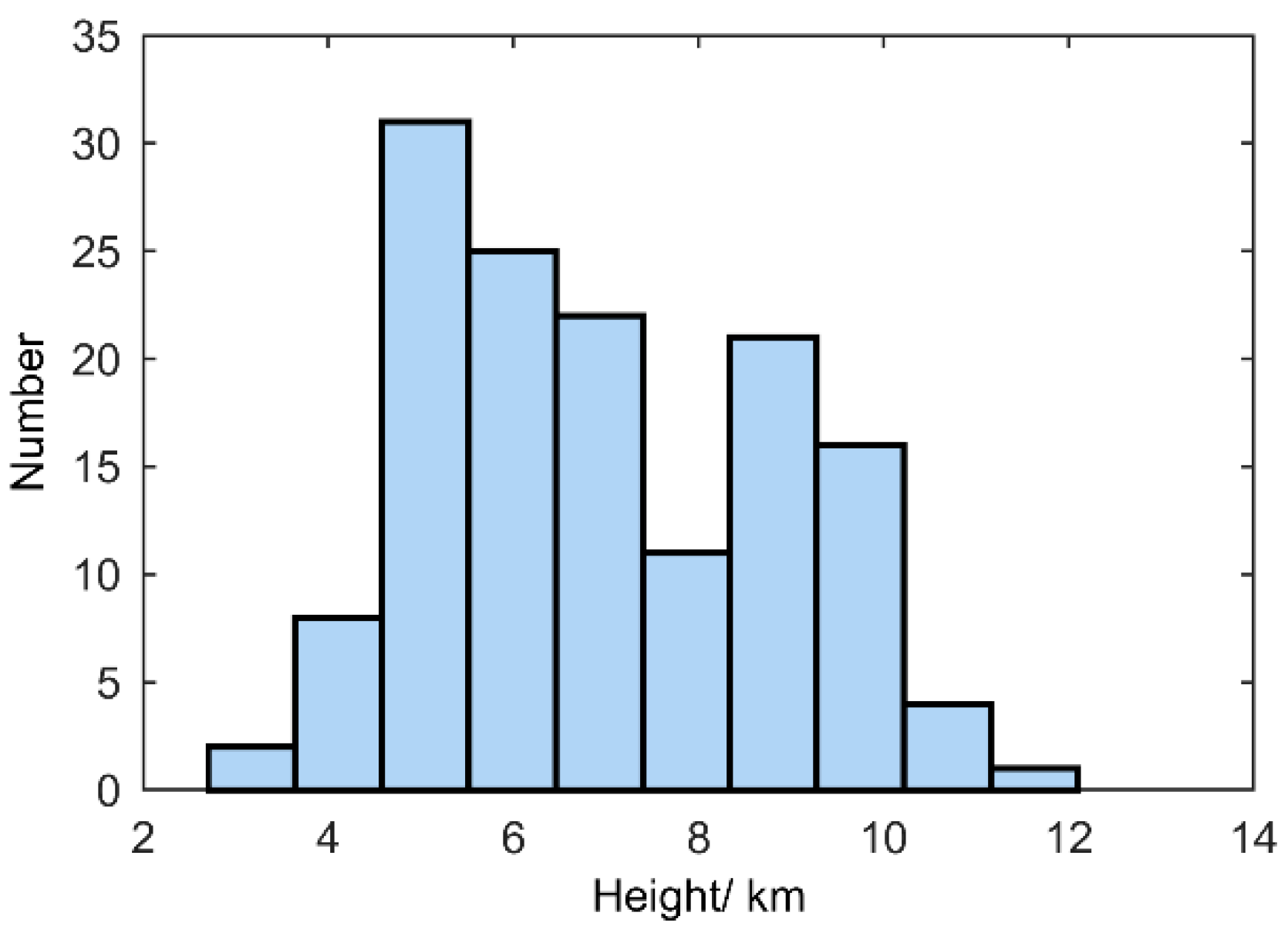
In addition to introducing the 3-D locating method using the 3-D locating results of one intra-cloud flash, the statistical results of the starting heights of 61 cloud-to-ground flashes and 80 intra-cloud flashes observed in the same year are also shown in Figure 7. Here, the lightning start time is defined as the time when the first pulse with an amplitude greater than 2 times the background noise occurs in a lightning-fast electric field record. If there are VHF 3-D locating results within 2 ms of the starting time of a lightning, it is considered that the lightning strike can be 3-D positioned from the starting. It can be seen that there are two distribution peaks in the distribution of lightning starting height, one appearing near the height of 5 km and the other near the height of 9 km. The results given here are very close to the initial height distribution of lightning observed by Procter in South Africa [41]. They are also consistent with the observations given by another TDOA lightning locating network [8,26,27,42]. The result also shows from one side that the 3-D lightning location observation given by this method is basically consistent with other VHF lightning location systems. The coincidence of the altitude of the lightning location reflects that the lightning origin height is closely related to the temperature stratification where the lightning occurs, and verifies the effect of the 3-D locating method from another angle.
5. Discussion and Conclusions
This paper introduces a two-station 3-D lightning location method for broadband interferometers. This method draws lessons from the high altitude wind speed observation of theodolite method used in the early days of meteorological observation, and has been modified according to the requirements of lightning location. The locating accuracy of this method is simulated and the actual observation results are given.
The simulation results of locating the accuracy of multi-station locating networks using the time difference of the arrival method can usually reach 200 m in the coverage area of the station network. There is also the problem that the locating accuracy decreases with the height of the radiation source. Taking the maximum station spacing as the diameter of the network coverage area, comparing the simulated 3-D locating accuracy, the simulated locating accuracy of the two-station interferometer is slightly lower than that of the multi-station TDOA network in the existing literature [43,44]. This is because there is a large error in the observation of the low elevation incident radiation source by the single-station interferometer. Therefore, the 3-D locating of the two-station interferometer is suitable for observing lightning with a close range and high elevation angle in a small area. Although this feature is not conducive to lightning observation for the entire thunderstorm process, it has little influence on the study of the temporal and spatial development characteristics of the single lightning discharge process. The combination of 3-D locating and single-station or double-station high time resolution 2-D locating results can make the temporal and spatial development characteristics of lightning discharge process more intuitive. When using 2-D locating data to analyze lightning discharge in a certain stage with high accuracy, the 3-D locating of the interferometer can provide a spatial position reference for it and help to combine it with other meteorological data such as radar.
Author Contributions
Software, H.L. and S.Q.; Supervision, W.D.; Writing–original draft, H.L.; Writing–review & editing, H.L. and S.Q. All authors were involved in designing and discussing the study. All authors have read and approved the final manuscript.
Funding
This research was funded by the National Key Research and Development Program of China (No. 2017YFC1501501), National Natural Science Foundation of China (No. 41405005), Basic Research Fund of Chinese Academy of Meteorological Sciences (No. 2016Y002) and the Ministry of Science and Technology (No. 2008EG137292).
Acknowledgments
The authors would like to thank Liangtao Xu, Biao Zhu, Hanbo Pan for their help with the experiments. The authors would like to thank the anonymous reviewers for their valuable comments.
Conflicts of Interest
The authors declare no conflict of interest.
Appendix A. The Principle of the Algorithm
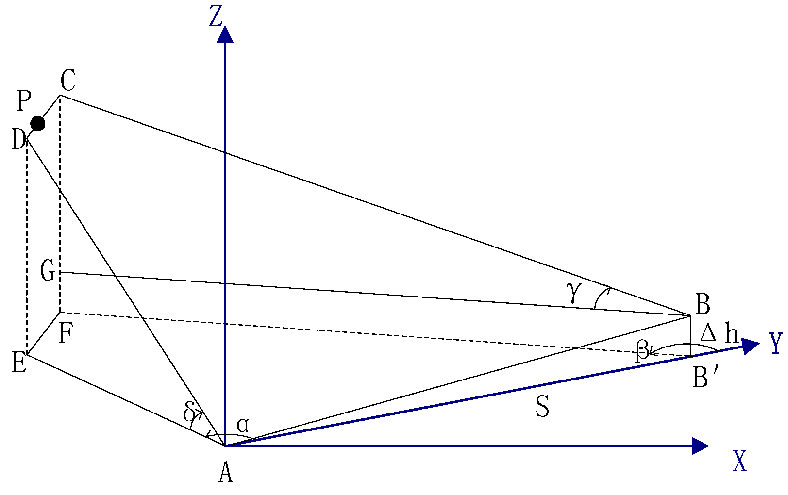
As shown in Figure A1, a coordinate system is established, site A is taken as the coordinate origin, and the projection of AB on the horizontal plane is the Y-axis. The azimuth angles of both sites are 0° in the positive direction of the Y-axis, increasing clockwise, with the positive direction of the X-axis pointing to 90°, and the Z-axis pointing vertically to the zenith. AD and BC are two rays along a certain azimuth angle (α, β) and elevation angle (δ, γ) of the two sites respectively, and CD is the common vertical line of the different plane line AD and BC. The radiation source is most likely to be located at a point p on the CD, and the position of the point p on the line segment CD is related to the length of AD and BC. The smaller the length, the closer the point p is to this end, satisfying . Thus, according to Figure A1, the 3-D coordinates of point p can be obtained by using the space vector relation. The following are the main derivation results:
Let the space vector of each line segment be expressed as
Then the coordinates of p (x, y, z) can be obtained from the following formula using the space vector relationship:
Since R3 is the mode of the common vertical line , the value of R3 can relatively reflect the error of each group of locating results, which can be used for the matching of radiation sources and the reliability analysis of locating results.
Figure A1.
The schematic diagram of a 3-D locating algorithm for two-station.

References
- Dwyer, J.R.; Uman, M.A. The physics of lightning. Phys. Rep. 2014, 534, 147–241. [Google Scholar] [CrossRef]
- Ismail, M.; Rahman, M.; Cooray, V.; Sharma, S.; Hettiarachchi, P.; Johari, D. Electric field signatures in wideband, 3 MHz and 30 MHz of negative ground flashes pertinent to Swedish thunderstorms. Atmosphere 2015, 6, 1904–1925. [Google Scholar] [CrossRef]
- Price, C. ELF electromagnetic waves from lightning: The schumann resonances. Atmosphere 2016, 7, 116. [Google Scholar] [CrossRef]
- Proctor, D.E. A hyperbolic system for obtaining VHF radio pictures of lightning. J. Geophys. Res. 1971, 76, 1478–1489. [Google Scholar] [CrossRef]
- Krehbiel, P.R.; Brook, M.; McCrory, R.A. An analysis of the charge structure of lightning discharges to ground. J. Geophys. Res. Oceans 1979, 84, 2432–2456. [Google Scholar] [CrossRef]
- Shao, X.M.; Krehbiel, P.R.; Thomas, R.J.; Rison, W. Radio interferometric observations of cloud-to-ground lightning phenomena in Florida. J. Geophys. Res. Atmos. 1995, 100, 2749–2783. [Google Scholar] [CrossRef]
- Shao, X.M.; Holden, D.N.; Rhodes, C.T. Broad band radio interferometry for lightning observations. Geophys. Res. Lett. 1996, 23, 1917–1920. [Google Scholar] [CrossRef]
- Rison, W.; Thomas, R.J.; Krehbiel, P.R.; Hamlin, T.; Harlin, J. A GPS-based three-dimensional lightning mapping system: Initial observations in central New Mexico. Geophys. Res. Lett. 1999, 26, 3573–3576. [Google Scholar] [CrossRef] [Green Version]
- Kawasaki, Z.; Mardiana, R.; Ushio, T. Broadband and narrowband RF interferometers for lightning observations. Geophys. Res. Lett. 2000, 27, 3189–3192. [Google Scholar] [CrossRef] [Green Version]
- Smith, D.A.; Eack, K.B.; Harlin, J.; Heavner, M.J.; Jacobson, A.R.; Massey, R.S.; Shao, X.M.; Wiens, K.C. The Los Alamos Sferic Array: A research tool for lightning investigations. J. Geophys. Res. Atmos. 2002, 107, 1–5. [Google Scholar] [CrossRef]
- Lyu, F.; Cummer, S.A.; Solanki, R.; Weinert, J.; McTague, L.; Katko, A.; Barrett, J.; Zigoneanu, L.; Xie, Y.; Wang, W. A low-frequency near-field interferometric-TOA 3-D Lightning Mapping Array. Geophys. Res. Lett. 2014, 41, 7777–7784. [Google Scholar] [CrossRef] [Green Version]
- Zhu, Y.; Rakov, V.; Tran, M. A study of preliminary breakdown and return stroke processes in high-intensity negative lightning discharges. Atmosphere 2016, 7, 130. [Google Scholar] [CrossRef]
- Zhao, P.; Zhou, Y.; Xiao, H.; Liu, J.; Gao, J.; Ge, F. Total lightning flash activity response to aerosol over china area. Atmosphere 2017, 8, 26. [Google Scholar] [CrossRef]
- Hettiarachchi, P.; Cooray, V.; Diendorfer, G.; Pichler, H.; Dwyer, J.; Rahman, M. X-ray Observations at Gaisberg Tower. Atmosphere 2018, 9, 20. [Google Scholar] [CrossRef]
- Wu, T.; Wang, D.; Takagi, N. Lightning mapping with an array of fast antennas. Geophys. Res. Lett. 2018. [Google Scholar] [CrossRef]
- Liu, X.; Krehbiel, P.R. The initial streamer of intracloud lightning flashes. J. Geophys. Res.: Atmos. 1985, 90, 6211–6218. [Google Scholar] [CrossRef]
- Mazur, V. Physical processes during development of lightning flashes. CR Phys. 2002, 3, 1393–1409. [Google Scholar] [CrossRef]
- MacGorman, D.R.; Rust, W.D.; Schuur, T.J.; Biggerstaff, M.I.; Straka, J.M.; Ziegler, C.L.; Mansell, E.R.; Bruning, E.C.; Kuhlman, K.M.; Lund, N.R.; et al. TELEX The thunderstorm electrification and lightning experiment. Bull. Am. Meteorol. Soc. 2008, 89, 997–1013. [Google Scholar] [CrossRef]
- Nag, A.; Rakov, V.A. Pulse trains that are characteristic of preliminary breakdown in cloud-to-ground lightning but are not followed by return stroke pulses. J. Geophys. Res. Atmos. 2008, 113, D1102. [Google Scholar] [CrossRef]
- Yoshida, S.; Biagi, C.J.; Rakov, V.A.; Hill, J.D.; Stapleton, M.V.; Jordan, D.M.; Uman, M.A.; Morimoto, T.; Ushio, T.; Kawasaki, Z.I. Three-dimensional imaging of upward positive leaders in triggered lightning using VHF broadband digital interferometers. Geophys. Res. Lett. 2010, 37, L05805. [Google Scholar] [CrossRef]
- Wu, T.; Yoshida, S.; Akiyama, Y.; Stock, M.; Ushio, T.; Kawasaki, Z. Preliminary breakdown of intracloud lightning: Initiation altitude, propagation speed, pulse train characteristics, and step length estimation. J. Geophys. Res.: Atmos. 2015, 120, 9071–9086. [Google Scholar] [CrossRef]
- Rison, W.; Krehbiel, P.R.; Stock, M.G.; Edens, H.E.; Shao, X.; Thomas, R.J.; Stanley, M.A.; Zhang, Y. Observations of narrow bipolar events reveal how lightning is initiated in thunderstorms. Nat. Commun. 2016, 7, 10721. [Google Scholar] [CrossRef] [PubMed] [Green Version]
- Stock, M.G.; Krehbiel, P.R.; Lapierre, J.; Wu, T.; Stanley, M.A.; Edens, H.E. Fast positive breakdown in lightning. J. Geophys. Res. Atmos. 2017, 122, 8135–8152. [Google Scholar] [CrossRef]
- Wu, B.; Zhang, G.; Wen, J.; Zhang, T.; Li, Y.; Wang, Y. Correlation analysis between initial preliminary breakdown process, the characteristic of radiation pulse, and the charge structure on the Qinghai-Tibetan Plateau. J. Geophys. Res. Atmos. 2016, 121, 412–434. [Google Scholar] [CrossRef]
- Xu, L.; Zhang, Y.; Liu, H.; Zheng, D.; Wang, F. The role of dynamic transport in the formation of the inverted charge structure in a simulated hailstorm. Sci. China Earth Sci. 2016, 59, 1414–1426. [Google Scholar] [CrossRef]
- Behnke, S.A.; Thomas, R.J.; Krehbiel, P.R.; Rison, W. Initial leader velocities during intracloud lightning: Possible evidence for a runaway breakdown effect. J. Geophys. Res. Atmos. 2005, 110, D10207. [Google Scholar] [CrossRef]
- Maggio, C.; Coleman, L.; Marshall, T.; Stolzenburg, M.; Stanley, M.; Hamlin, T.; Krehbiel, P.; Rison, W.; Thomas, R. Lightning-initiation locations as a remote sensing tool of large thunderstorm electric field vectors. J. Atmos. Ocean. Technol. 2005, 22, 1059–1068. [Google Scholar] [CrossRef]
- Mazur, V.; Williams, E.; Boldi, R.; Maier, L.; Proctor, D.E. Initial comparison of lightning mapping with operational time-of-arrival and interferometric systems. J. Geophys. Res. Atmos. 1997, 102, 11071–11085. [Google Scholar] [CrossRef] [Green Version]
- Stock, M.G.; Akita, M.; Krehbiel, P.R.; Rison, W.; Edens, H.E.; Kawasaki, Z.; Stanley, M.A. Continuous broadband digital interferometry of lightning using a generalized cross-correlation algorithm. J. Geophys. Res. Atmos. 2014, 119, 3134–3165. [Google Scholar] [CrossRef] [Green Version]
- Liu, H.; Dong, W.; Wu, T.; Zheng, D.; Zhang, Y. Observation of compact intracloud discharges using VHF broadband interferometers. J. Geophys. Res. Atmos. 2012, 117, D1203. [Google Scholar] [CrossRef]
- Qiu, S.; Zhou, B.; Shi, L. Synchronized observations of cloud-to-ground lightning using VHF broadband interferometer and acoustic arrays. J. Geophys. Res. 2012, 117, D19204. [Google Scholar] [CrossRef]
- Wansheng, D.; Xinsheng, L.; Ye, Y. Broadband interferometer observations of a triggered lightning. Chin. Sci. Bull. 2001, 46, 1561–1565. [Google Scholar]
- Qiu, S.; Zhou, B.H.; Shi, L.H.; Dong, W.S.; Zhang, Y.J.; Gao, T.C. An improved method for broadband interferometric lightning location using wavelet transforms. J. Geophys. Res. 2009, 114, 1–9. [Google Scholar] [CrossRef]
- Yoshihashi, S.; Kawasaki, I.; Matsuura, K.; Isoda, H.; Sonoi, Y. 3D imaging of lightning channel and leader progression velocity. Electr. Eng. Jpn. 2001, 137, 22–28. [Google Scholar] [CrossRef]
- Li, Y.; Qiu, S.; Shi, L.; Huang, Z.; Wang, T.; Duan, Y. Three-Dimensional Reconstruction of Cloud-to-Ground Lightning Using High-Speed Video and VHF Broadband Interferometer. J. Geophys. Res. Atmos. 2017, 122, 413–420, 435. [Google Scholar] [CrossRef]
- Takeshi Morimoto, Z.K. VHF broadband digital interferometer. IEEJ Trans. Electr. Electron. 2006, 1, 140–144. [Google Scholar] [CrossRef] [Green Version]
- Ushio, T.; Kawasaki, Z.I.; Ohta, Y.; Matsuura, K. Broad band interferometric measurement of rocket triggered lightning in japan. Geophys. Res. Lett. 1997, 24, 2769–2772. [Google Scholar] [CrossRef]
- Kawada, M. Fundamental study on location of a partial discharge source with a VHF-UHF radio interferometer system. Electr. Eng. Jpn. 2003, 144, 32–41. [Google Scholar] [CrossRef]
- Stock, M.; Krehbiel, P. Multiple baseline lightning interferometry—Improving the detection of low amplitude VHF sources. In Proceedings of the International Conference on Lightning Protection, Shanghai, China, 11–18 October 2014; pp. 293–300. [Google Scholar]
- Thyer, N. Double Theodolite Pibal Evaluation by Computer. J. Appl. Meteorol. 2010, 1, 66–68. [Google Scholar] [CrossRef]
- Proctor, D.E. Regions where lightning flashes began. J. Geophys. Res. Atmos. 1991, 96, 5099–5112. [Google Scholar] [CrossRef]
- Marshall, T.C.; Stolzenburg, M.; Maggio, C.R.; Coleman, L.M.; Krehbiel, P.R.; Hamlin, T.; Thomas, R.J.; Rison, W. Observed electric fields associated with lightning initiation. Geophys. Res. Lett. 2005, 32, L3813. [Google Scholar] [CrossRef]
- Thomas, R.J.; Krehbiel, P.R.; Rison, W.; Hunyady, S.J.; Winn, W.P.; Hamlin, T.; Harlin, J. Accuracy of the Lightning Mapping Array. J. Geophys. Res. Atmos. 2004, 109, D14207. [Google Scholar] [CrossRef]
- Yoshida, S.; Wu, T.; Ushio, T.; Kusunoki, K.; Nakamura, Y. Initial results of LF sensor network for lightning observation and characteristics of lightning emission in LF band. J. Geophys. Res. Atmos. 2014, 119, 12–34, 51. [Google Scholar] [CrossRef]
Figure 1.
The 2-D locating calculation flow chart.

Figure 2.
The schematic diagram of the radiation point matching algorithm.

Figure 3.
The locating error distribution map at different heights. (a) 10 km height; (b) 7 km height; (c) 5 km height; (d) 2 km height. The unit of locating error is “km”.
Figure 3.
The locating error distribution map at different heights. (a) 10 km height; (b) 7 km height; (c) 5 km height; (d) 2 km height. The unit of locating error is “km”.

Figure 4.
The two-station 2-D locating results of an IC flash. (a1) the fast electric field change waveform observed by site A; (b1) elevation angle change with time observed by site A; (c1) azimuth angle change with time observed by site A; (d1) azimuth versus elevation 2-D images observed by site A. (a2) the fast electric field change waveform observed by site B; (b2) elevation angle change with time observed by site B; (c2) azimuth angle change with time observed by site B; (d2) azimuth versus elevation 2-D images observed by site B.

Figure 5.
The 3-D locating results of an IC flash. (a) The fast electric field change waveform observed by site A; (b) the change of the radiation source height with time; (c) the projection of the 3-D locating result on the X-Z plane; (d) 3-D locating result and the two observation sites (e) the projection on the X-Y plane; (f) the projection on the Y-Z plane.

Figure 6.
R1, R2 and R3 corresponding to the locating result. (a) Values of R1, R2, and R3 versus the positioning result serial number; (b) Statistical results of R3.
Figure 6.
R1, R2 and R3 corresponding to the locating result. (a) Values of R1, R2, and R3 versus the positioning result serial number; (b) Statistical results of R3.

Figure 7.
The lightning initiation height distribution is given by a two-station 3-D locating algorithm.
Figure 7.
The lightning initiation height distribution is given by a two-station 3-D locating algorithm.

© 2018 by the authors. Licensee MDPI, Basel, Switzerland. This article is an open access article distributed under the terms and conditions of the Creative Commons Attribution (CC BY) license (http://creativecommons.org/licenses/by/4.0/).
Share and Cite
MDPI and ACS Style
Liu, H.; Qiu, S.; Dong, W. The Three-Dimensional Locating of VHF Broadband Lightning Interferometers. Atmosphere 2018, 9, 317. https://doi.org/10.3390/atmos9080317
AMA Style
Liu H, Qiu S, Dong W. The Three-Dimensional Locating of VHF Broadband Lightning Interferometers. Atmosphere. 2018; 9(8):317. https://doi.org/10.3390/atmos9080317
Chicago/Turabian StyleLiu, Hengyi, Shi Qiu, and Wansheng Dong. 2018. "The Three-Dimensional Locating of VHF Broadband Lightning Interferometers" Atmosphere 9, no. 8: 317. https://doi.org/10.3390/atmos9080317
Note that from the first issue of 2016, this journal uses article numbers instead of page numbers. See further details here.