Modeling Wildfire Smoke Pollution by Integrating Land Use Regression and Remote Sensing Data: Regional Multi-Temporal Estimates for Public Health and Exposure Models

Abstract

To understand the health effects of wildfire smoke, it is important to accurately assess smoke exposure over space and time. Particulate matter (PM) is a predominant pollutant in wildfire smoke. In this study, we develop land-use regression (LUR) models to investigate the impact that a cluster of wildfires in the northwest USA had on the level of PM in southern Alberta (Canada), in the summer of 2015. Univariate aerosol optical depth (AOD) and multivariate AOD-LUR models were used to estimate the level of PM_2.5 in urban and rural areas. For epidemiological studies, it is also important to distinguish between wildfire-related PM_2.5 and PM_2.5 originating from other sources. We therefore subdivided the study period into three sub-periods: (1) Pre-fire, (2) during-fire, and (3) post-fire. We then developed separate models for each sub-period. With this approach, we were able to identify different predictors significantly associated with smoke-related PM_2.5 verses PM_2.5 of different origin. Leave-one-out cross-validation (LOOCV) was used to evaluate the models’ performance. Our results indicate that model predictors and model performance are highly related to the level of PM_2.5, and the pollution source. The predictive ability of both uni- and multi-variate models were higher in the during-fire period than in the pre- and post-fire periods.

1. Introduction

Fire smoke is a complex mixture of gases and particles, including carbon dioxide (CO₂), methane (CH₄) and nitrogen dioxide (NO₂), that are known as greenhouse gases, as well as high levels of particulate matter (PM), toxins, carbon monoxide (CO), ozone (O₃), and benzene [1]. Thus, fire smoke is a significant contributor to air pollution. It impacts climate as well, through primary emission of greenhouse gases and aerosol (direct impact), and through secondary effects on atmospheric chemistry (indirect impact) [2]. Wildfire smoke is associated with adverse health effects (both long-term and short-term) on exposed human population, and it contributes to annual global premature mortality [3,4,5]. Individuals are affected by fire smoke differently: At-risk groups include people suffering from respiratory disease such as asthma or lung cancer, people with an existing heart condition, children, people over 65, and pregnant women [6].

To understand health-related effects, it is important to accurately assess wildfire smoke exposure. Particulate matter (PM) is a predominant air pollutant in wildfire smoke [7], and it poses the most significant risk to public health [6]. PM is a mixture of solid particles and liquid droplets found in the air, and its physical and chemical characteristics vary by location. Common chemical constituents of PM include sulfates, nitrates, ammonium, other inorganic ions such as ions of sodium, potassium, calcium, magnesium, and chloride, organic and elemental carbon, crustal material, particle-bound water, metals, and polycyclic aromatic hydrocarbons (PAH) [8]. PM also contains biological components, such as allergens, and microbial compounds [8]. These fine particles have various environmental effects, including reducing visibility, changing surface temperatures by preventing sunlight from reaching the ground, changing cloud properties by acting as cloud condensation nuclei (CCN), and, more importantly, becoming a health hazard [9].

Forest fires are a natural occurrence in forest ecosystem, important for maintaining the health and diversity of forest. At the same time, they can be harmful when they threaten communities directly, or through smoke. Recent intensification of wildfire frequency and severity has triggered an increasing interest in quantifying smoke exposure for application in public health studies. On average, Canada has about 7500 fires a year, and the frequency and severity of forest fires is increasing due to climate change [10].

Location is an important dimension of wildfire, wildfire smoke, and PM chemistry. With increasing likelihood of wildfire occurrence, it is essential to characterize wildfire smoke and associated PM. Estimating spatial and multi temporal patterns of PM related to wildfire smoke is key to accurately assessing exposure of specific populations, groups, and communities. Accurate and reliable models to estimate spatio-temporal distribution of particulate matter can not only feed epidemiological models, but also yield timely information for public health during wildfire events.

The present study investigates the impacts that a cluster of wildfires in the northwest United States of America (USA) had on the level of particulate matter in southern Alberta (Canada). The main wildfire event occurred in Washington State (USA) in August 2015, and was widely publicized in North America as the Pacific Northwest (PNW) wildfire [11]. The PNW wildfire began in mid-August 2015 and led to smoke exposure in southern Alberta in the week of 23 August. PM concentration returned to background levels by 1 September 2015.

Estimation of fire smoke exposure with relatively high spatial resolution is usually challenging due to the limitations of the measuring instruments and estimation methods. In general, the main problem is the scarcity of air quality stations: PM_2.5 records are too few to estimate the exposure of an entire population. Furthermore, most stations are point-based, that is, they are not designed to capture the spatial extent of PM_2.5 related to fire smoke.

Many studies have estimated the impact of ambient air pollution and human exposure to wildfire smoke at the population level [12,13,14,15]. Methods commonly used to quantify such exposure include ground-based air quality stations [12,13], land use regression (LUR) [16,17,18,19,20], remote sensing or aerosol optical depth (AOD) based models [21,22,23,24], chemical transfer models (CTM) [14,25], mixed-effect models (MEM) [26,27], multiple linear regression (MLR) [9,28,29,30], geostatistical spatial interpolation methods (Kriging) [31,32,33], and geographically weighted regression (GWR) [34,35].

Satellite observations can be used to assess PM_2.5 exposure based on satellite AOD retrievals. Satellites provide observations over spatially extensive areas, which could be a suitable complement to ground-based measurements in wildfire smoke exposure studies [36]. AOD is a measure of the extinction of electromagnetic radiation due to available aerosol in the atmosphere. Its use has increased over the past decade [9,21,22,23,37,38,39]. AOD is a function of aerosol mass concentration, where higher AOD values correspond to higher aerosol concentration [40]. For this reason, AOD can be used to estimate PM_2.5. Different models have been used to assess the relationship between AOD and PM_2.5, including simple linear regression [41], multiple linear regression utilizing satellite AOD among other covariates (e.g., humidity, wind speed, temperature, aerosol type, and boundary layer height) [28,29,42,43,44]. There is not a perfect correlation between AOD and PM_2.5, because PM_2.5 is a measure of near-surface particle mass that concentrates near the surface, while AOD represents the aerosol content distributed within a column of air from the Earth to the top of the atmosphere [45]. Remote sensing observations, including AOD images, provide extensive spatial coverage and reliable repeated measurements. However, there are some limitations with AOD images. For example, cloudy days are a major problem with remotely sensed methods of PM_2.5 estimation [24], as they limit the number of days available for analysis.

A variety of satellite sensors provide AOD image including Moderate Resolution Imaging Spectrometer (MODIS), the Ozone Monitoring Instrument (OMI), the Multi-Angle Imaging Spectrometer (MISR), the Geostationary Operational Environment Satellite (GEOS), Polarization of Earth’s Reflectance and Directionality (POLDER), the Sea-viewing Wide Field-of-view Sensor (SeaWiFS), and the Cloud-Aerosol Lidar with Orthogonal Polarization (CALIOP). AOD is affected by ambient conditions, such as humidity and vertical profile, as well as chemical properties of the atmosphere [45].

Land use regression (LUR) methods estimate pollution concentration at a given location using surrounding attributes, such as land use type and traffic characteristics within a surrounding area, as predictors [33]. LUR is generally used to estimate air pollution at fine spatial scales, and can be used to assign household-level exposure in community health studies [20]. Based on the type of the pollutant and the source of the air pollution different land use variables can be used in LUR. For example, road types, parks, residential, commercial, and industrial land uses have been used by Bertazzon et al. (2015), for modeling urban air pollution [20]. Yang et al. (2017) developed LUR to estimate PM_2.5 and NO₂ using different land use types including cultivated land, forest, grassland, shrub and water land, and traffic and urbanization [46]. According to a report by Environment and Climate Change Canada (2017), the main sources of PM_2.5 emission in Canada include dust and fire, agriculture, home firewood burning, mineral and oil and gas industry, transportation, and building utilities [47]. Different specifications of LUR (ordinary least squares (OLS) regression, geographically weighted regression (GWR), and spatial autoregression (SAR)) have been employed to predict air pollution in different studies [20,38,48].

Different factors affect the identification of the most reliable models in different wildfire events and areas. As each model has strengths and weaknesses, no single model can be considered the most accurate to quantify human exposure to wildfire smoke [44]. For example, ground-based measurements provide accurate information for each station; however, the spatial density of station distribution is not sufficient to estimate the spatial distribution of wildfire smoke. GWR is suitable on a reginal scale and needs small amounts of data; however, its performance depends on ground-based measurements. Therefore, in areas lacking air quality (AQ) stations, GWR is not reliable [44]. CTM can predict pollutant concentration without ground based measurements [49]. However, collecting the necessary chemical and physical information is time consuming and requires financial resources [50]. Although MLR has relatively weak predictability, it can be improved by adding some covariates [44]. For example, for estimating PM_2.5 using AOD aerosol type, methodological and land use variables may be included in the regression to improve the model performance [28,51,52]. MEM performance is usually strong, and the R² value could reach up to 0.80 [27,53]. The main disadvantage of this method is that, if ground-based stations are not available in some areas, the model assumptions are not met, potentially affecting its performance [54]. In addition, there are differences between models trained for smoke-based PM_2.5 (i.e., when the wildfire is the source of PM_2.5), and models developed to estimate PM_2.5 from other sources, mainly of industrial and transportation origin.

In the present study, the model choice was affected by many factors, including the number of ground-based AQ monitors, the characteristics of the study area, data availability, data uncertainty, and the significance of spatial autocorrelation in the data. Experiments with a range of predictors showed that the predictors associated with PM_2.5 could change even over a short period (two months), depending on the source of PM_2.5. The predictors considered include spatial and temporal variables, such as wind speed and land use variables, and satellite data, including AOD and (normalized difference vegetation index). Roadway and industrial variables are established predictors in LUR models for estimating air pollution [17,19,55], whereas satellite observations are relatively uncommon. In the present study, we investigated the role of vegetation on the level of PM_2.5 concentration during a wildfire event. Plants have the ability to reduce some of air pollution particles as plant leaves and stems increase surface areas to which airborne particles can be absorbed [56]. NDVI is an index of greenness, vegetation, and agriculture land use that has been rarely used as a predictor in LUR models [57,58,59,60]. Wu et al., [57] investigated the role of surrounding greenness on intra urban PM_2.5 variability, showing that there was a strong negative correlation (ranging between −0.71 and −0.77) between NDVI and PM_2.5.

To examine the temporal variability in predictors, we divided the study period into the following three sub-periods. “Pre-fire period”, that is, when the level of PM_2.5 in the study area was normal (the average level of the 24-h PM_2.5 was lower than the standard level: 30 µg/m³ [60]); “during-fire” period, that is, when the concentration of PM_2.5 was dramatically increased in the majority of AQ stations located in the study area; “post-fire" period, that is, when the PM_2.5 concentration returned to background levels. The subdivision of the study period into three separate sub-periods allowed us to test different models for the same study area, yet with very different PM_2.5 concentration levels and pollutant sources over two months. The study area covers most of southern Alberta, including urban and rural areas. Rural areas usually have insufficient AQ monitors and most epidemiological studies are limited to urban areas. We propose an extension of the models to rural areas to estimate levels of smoke-based PM_2.5 concentration in areas where AQ monitors are not enough or available.

In the present study, we estimate two types of predictive models: univariate models based on satellite AOD; and integrated AOD-LUR models. Both models yield estimates of PM_2.5 for each of the sub-periods in August and September 2015 over the whole urban and rural southern Alberta.

2. Materials and Methods

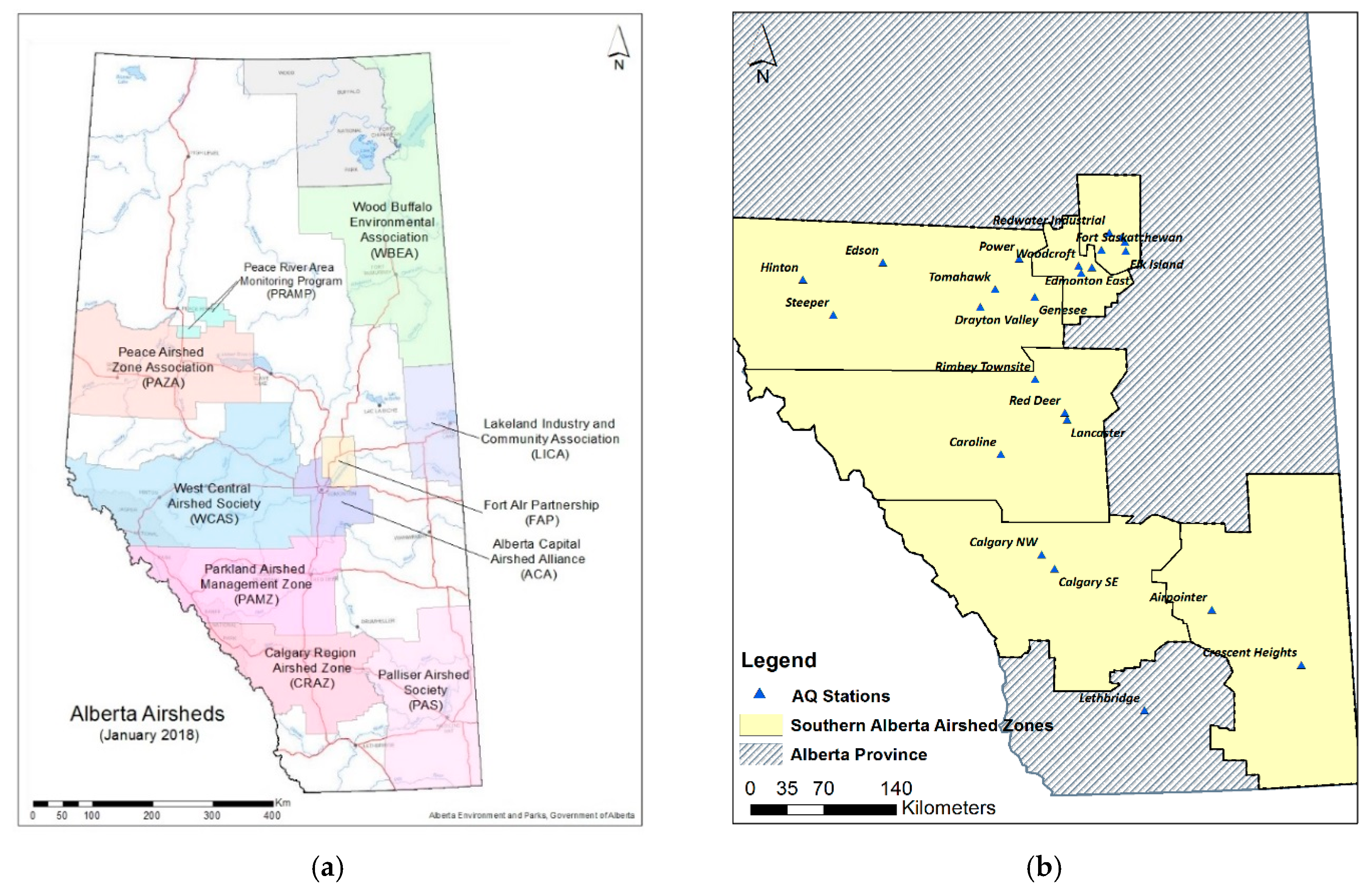
2.1. Study Area and Ground-Level PM_2.5 Measurements (Dependent Variable)

The study area covers the southern part of the province of Alberta (Canada). The Clean Air Strategic Alliance (CASA) was established to manage air quality in Alberta. Ten Airshed zones were formed between 1996 and 2017; the study area includes six of these zones: Alberta Capital Airshed (ACA), Calgary Region Airshed Zone (CRAZ), Fort Air Partnership (FAP), Palliser Airshed Society (PAS), Parkland Airshed Management Zone (PAMZ), and West Central Airshed Society (WCAS) (Figure 1). The Airshed zones now operate more than 70 air monitoring stations across the Province.

Twenty-four-hour PM_2.5 concentrations were collected at 24 Alberta Airshed Zones continuous AQ stations (Figure 1b) for the months of August and September 2015 (http://airdata.alberta.ca/RelatedLinks.aspx). The daily PM_2.5 concentrations were averaged for each period in each station.

2.2. Temporal (Meteorological) and Spatial Predictors

Wind speed and direction were collected at each monitoring station. A windrose was created using four quadrants, defined by radii traced at 0, 90, 180, and 270 degrees, so that each quadrant is centered on the northeast, southeast, southwest, and northwest directions, respectively. As the fire source is located southwest of the study area, based on the recorded wind direction, hourly wind speed, the southwest quadrant of each station was averaged over each of the three sub-periods. Average humidity and temperature over each period were obtained from continuous weather stations as well.

Industrial and road length predictors were generated by drawing circular buffers around each monitoring station. Following the previous studies [20], the buffers for industrial variables ranged from 5000 to 10,000 m and for road length from 500 to 1000 m. The number of industrial emission points and length of road in each buffer were calculated. The Alberta road network was acquired from the National Road Network (NRN) [61], and industrial points were obtained from the National Pollutant Release Inventory (NPRI) [62].

Elevation data were acquired through an Alberta DEM (digital elevation model) from DMTI Spatial [63]: Contour lines, stored in a shapefile, were converted to a raster file of elevation values, using ESRI ArcMap 10.3.1.

As the 2015 PNW wildfire originated in Washington State, USA, the centroid of the fire was digitized in ArcGIS as a source of the smoke over Alberta. The Euclidean distance between each AQ station in the study area and the source of the fire was calculated.

2.3. Satellite Data

2.3.1. Satellite AOD Images

One of the most common satellite products used in the field of air quality is aerosol optical depth (AOD), a quantity that indicates the amount of aerosol particles in the atmosphere. In our study, AOD data were derived from both MODIS and ozone monitoring instrument (OMI).

Averaged MOD 08 product of MODIS (at 1 degree resolution) and OMI/Aura AOD data (at 0.25 degree resolution) were collected from the NASA Giovanni website [64] for the three sub-periods (pre-, during, and after-fire) of the study.

2.3.2. NDVI

Normalized Difference Vegetation Index (NDVI) has been used as greenness predictor in previous air pollution studies [57,58,59,60]. NDVI is an image-based greenness index for measuring and monitoring density of plant, vegetation and biomass production on the earth. The NDVI values range is from −1 to +1. Increasing positive NDVI values indicate increasing amount of healthy vegetation and correspond to dense vegetation. Areas covered by rock, sand, snow, and non-vegetative features show very low NDVI values (close to -1).

Global NDVI is one of the vegetation products of MODIS that contains atmospherically corrected bi-directional surface reflectance. Global NDVI data are provided every 16 or 30 days. In the present study, MOD13C2 data (monthly NDVI image) were downloaded from the NASA Giovanni website [64]. Considering that the NDVI is not expected to change significantly over a month we collected one image for August 2015 and one for September 2015. Those monthly NDVI images were projected on a 0.05 degrees geographic Climate Modeling Grid (CMG).

2.4. PM_2.5 Predictive Models

In the present study, a univariate model was first tested, using AOD as the single predictor, to assess the amount of variability of PM_2.5 concentration that can be modeled by AOD for different pollution levels in each sub-period. Subsequently, this simple model was integrated into a LUR model by including traditional land use variables (Equation (1)) [20], as well as meteorological variables. The purpose of this integration was to improve the model’s spatial and temporal fit, as the relationship between AOD and PM_2.5 is thought to be affected by other variables. Furthermore, the latter model tests the association of PM_2.5 with relevant predictors. An AOD-LUR multivariate model was independently estimated for each sub-period. Model selection led to the identification of different sets of significant predictors, yielding respective coefficients for each sub-period.

Traditional LUR models are defined as:

$$y_i={\beta }_0+{\displaystyle \sum }_k{\beta }_k{x}_{ik}+{\epsilon }_i$$

(1)

where the response variable, y, (e.g., PM_2.5) indicates pollution concentration at location i, (where each i is a sample AQ station), and is expressed as a function of k attributes, or independent variables (x), such as land use variables and traffic characteristics [33]. Coefficients are estimated using the ordinary least squares (OLS) estimation method.

Variable selection was conducted independently for each sub-period model; over twenty variables were tested in the prediction models, including spatial predictors (land use type, industrial, and transportation indicators), temporal predictors (meteorology) and remotely sensed data (AOD and NDVI). Model selection was based on theoretical relevance and statistical significance. First, the most relevant variables were chosen for initial list in each period. Then, forward stepwise multiple linear regression and subset regression methods were used to identify the most significant predictors in each model. Global Moran’s I [65] was used to identify spatial clustering and autocorrelation at the spatial variables, i.e., PM_2.5, land use variables, and satellite observations recorded at each AQ station. Residual Moran’s I and Lagrange multiplier (LM) test [66] were used to assess the spatial autocorrelation in the residuals of each sub-period model.

After estimating the best prediction model for each sub-period, the regression coefficients were applied to calculate PM_2.5 in the centroid of each 10 by 10 km grid-cell overlaying the study area. Then inverse distance weighted (IDW) interpolation technique was applied to map the calculated PM_2.5 level between grid centers. IDW works on the assumption that near things are more alike than things that are farther apart. Using the estimated value at each grid center, IDW predicts a value for any unknown location, giving greater weights to points closer to the known location. The weights are determined by distance [67]. A summary of variables, their names, and additional details are shown in

Table 1. Response (PM_2.5) and predictor variables including satellite data, spatial and temporal variables used in variable selection procedure.

Response Variable	Name	Unit
PM2.5	Particulate Matter 2.5	µg/m3
Satellite Data	Name	Spatial Resolution	Temporal Resolution
Vegetation Index	NDVI-30 days	0.05 degree	Monthly
Aerosol optical depth (MODIS)	AOD_MODIS	1 degree	Daily (averaged to study period)
Aerosol optical depth (OMI)	AOD_OMI	0.25 degree	Daily (averaged to study period)
Spatial Variables	Name	Unit	Circular Buffer/Scale
Distance to the source of fire	Dis	kilometer	-
Land use: Industrial	LU_ind	count	5000–10,000 m
roads	Road	meter	500–1000 m
Temporal Predictors	Name	Unit	Resolution
Relative Humidity	RH		Hourly (averaged to study period)
Temperature	Temp	Celsius	Hourly (averaged to study period)
Wind speed (southwest)	WS	km/h, at 10 m height	Hourly (averaged in southwest direction)

. Performance of the models in the PM_2.5 concentration estimation is evaluated by using different statistical indices including coefficient of determination (R²), adjusted coefficient of determination (adj R²), cross-validated R² (CV-R²), RMSE, CV-RMSE, and Akaike information criterion (AIC).

2.5. Validation

The validity of the AOD-based and AOD_LUR models used for estimation of PM_2.5 concentration was evaluated by a cross-validation procedure. As the total number of AQ stations (PM_2.5 samples) was too small to divide the data set to test and train separately, we applied leave-one-out cross validation (LOOCV) procedure. With this method, each PM_2.5 measurements are estimated based on a model calibrated over the other PM_2.5 measurements. Therefore, in this study, for each period, we developed almost 24 individual models (after removing outliers we had 22 data for pre-fire period, 24 data for during-fire period, and 23 data for post-fire period). Then the cross-validated root mean square error (CV-RMSE) and CV-R² were calculated for validating the models. The structure of the model (the variables in the model) was the same as the one used in the full training dataset (the model trained by 24 PM_2.5 measurements) but the coefficients of the model changed.

3. Results

Table 2. Descriptive statistics of PM_2.5 concentration over three periods.

PM2.5 (µg/m3)	N	Max	Mean	Min	S.D.	Moran’s I	P(I)
Period 1 (Pre-Fire)	22	14	6.2	3.2	2.4	0.08	0.1
Period 2 (During-Fire)	24	51.5	19.5	6	12.9	0.55	0.00
Period 3 (Post-Fire)	23	9.8	4.2	0.8	2.1	0.01	0.28

shows the descriptive statistics of PM_2.5 concentration over the three sub-periods. The overall mean concentration of PM_2.5 over the during-fire period is significantly higher than the pre- and post-fire periods (i.e., 19.5 µg/m³ compared to 6.2 µg/m³ and 4.2 µg/m³, respectively). Global Moran’s I tests indicate that there was no significant spatial autocorrelation in the measured PM_2.5 at AQ stations in any of the sub-periods over the study area.

The temporal daily variability of PM_2.5 level at each of the 24 AQ stations during the whole period (1 August to 30 September) is shown in Figure 2. The recorded concentrations of PM_2.5 increased greatly in late August. Calgary monitors reported the level of PM_2.5 as about 170 µg/m³ on 25 August, which is, more than three times their typical peak in non-smoke days. It can be seen in this figure that the daily averaged PM_2.5 level for some stations was more than 80 µg/m³ on 25 August. By 1 September, the PM_2.5 concentration returned to the background level.

The spatial variability of PM_2.5 concentration was estimated using AOD and AOD-LUR models during the three sub-periods. That is, two models were developed for each period. The univariate AOD models are summarized in

Table 3. Results of aerosol optical depth (AOD)-based model for three periods.

Predictors	Period 1: Pre-Fire (1–23 August 2015)				Period 2: During-Fire (24–31 August 2015)				Period 3: Post-Fire (1–30 September 2015)
	Coefficient	Std. Error		p-Value	Coefficient	Std. Error		p-Value	Coefficient	Std. Error		p-Value
Intercept	4.165	0.58		0.00	4.512	3.77		0.24	0.73	0.35		0.05
AOD	7.76	2.65		0.00	18.154	3.93		0.00	6.75	4.47		0.14
	Index/Test		Adjust/p-Value		Index/Test		Adjust/p Value		Index/Test		Adjust/p Value
R2	0.29		0.26		0.50		0.47		0.13		0.05
CV-R2	0.25		-		0.40		-		0.12		-
Moran’s I	0.09		0.05		0.05		0.07		−0.03		0.37
LMerr	0.54		0.46		0.23		0.62		0.08		0.76
RMSE	1.4		-		9		-		0.51		-
CV-RMSE	1.39		-		9.8		-		0.6		-
AIC	78		-		179		-		41		-

, and the multivariate AOD-LUR models in

Table 4. Results of aerosol optical depth–land-use regression (AOD-LUR) model for three periods.

Predictors	Period 1: Pre-Fire (1–23 August 2015)				Period 2: During-Fire (24–31 August 2015)				Period 3: Post-Fire (1–30 September 2015)
	cor 1 (%)	Coefficient	Std. Error	p-Value	cor (%)	Coefficient	Std. Error	p-Value	cor (%)	Coefficient	Std. Error	p-Value
Intercept	-	3.84	0.58	0.00	-	63.38	13.08	0.00	-	1.55	0.44	0.00
AOD	0.50	4.82	2.75	0.09	0.70	12.71	3.00	0.00	-	-	-	-
NDVI	-	-	-	-	0.60	−32.95	9.61	0.00	-	-	-	-
Distance	-	-	-	-	0.61	−5.6 × 10−5	0.00	0.00	-	-	-
Elevation	-	-	-	-	-	-	-	-	0.35	−9.61 × 10−4	0.00	0.05
Road_1km	0.55	6.8 × 10−5	0.00	0.00	-	-	-	-	0.50	1.87 × 10−5	0.00	0.00
LU_ind_5km	-	-	-	-	-	-	-	-	0.51	2.9 × 10−2	0.01	0.08
	Index/Test		Adjust/p-Value		Index/Test		Adjust/p-Value		Index/Test		Adjust/p-Value
R2	0.50		0.45		0.77		0.74		0.54		0.47
CV-R2	0.41		-		0.71		-		0.42		-
Moran’s I	−0.028		0.35		0.04		0.01		−0.16		0.83
LMerr	0.051		0.82		0.12		0.72		1.84		0.17
RMSE	1.17		-		6		6.8		0.36		-
CV-RMSE	1.34		-		7.06		-		0.44		-
AIC	77		-		162		-		29		-

¹: Correlation between PM_2.5 and predictors in each period.

. The final equation of the multivariate model for each sub-period is as follows:

Pre-fire period model:

$$y_i=3.84+\left(4.82\times AOD\right)+\left(6.8\times {10}^{-5}\times {\mathrm{Road}}_{1\mathrm{km}}\right)$$

(2)

During-fire period model:

$$y_i=63.38+\left(12.71\times AOD\right)+\left(-32.95\times \mathrm{NDVI}\right)+\left(-5.656\times {10}^{-5}\times \mathrm{Dist}\right)$$

(3)

Post-fire period model:

$$\log (y_i)=1.55+\left(-9.61\times {10}^{-4}\times Elevation\right)+\left(1.87\times {10}^{-5}\times {\mathrm{Road}}_{1\mathrm{km}}\right)+\left(2.9\times {10}^{-2}\times \mathrm{LU}\_\mathrm{ind}{\_}_{5\mathrm{km}}\right)$$

(4)

As it is shown in the above equations, there are substantial differences between the intercept values across multivariate models. The highest intercept value was obtained for the during-fire period, due to the higher level of PM_2.5 concentration in that period. The lowest intercept was obtained for the post-fire period, as we applied a logarithmic transformation to PM_2.5 to normalize the PM_2.5 distribution and improve the results.

The model results shown in Table 3 for all three sub-periods indicate that the goodness-of-fit of the univariate AOD model was limited, especially for the pre- and post-fire periods, that is, when the PM_2.5 level was low. The goodness-of-fit for all three sub-periods improves substantially by adding temporal and spatial variables to each regression (Table 4). The LUR was developed for each period using different image-based, temporal, and spatial variables. The only significant variable, beside AOD, in the pre-fire model is “road length within a 1000-m buffer”. With the addition of this variable, the model R² increased from 0.29 to 0.50. For the during-fire model, the significant variables, besides AOD, were “NDVI”, and “distance to fire. The integration of AOD with distance to the fire period and NDVI improved model performance substantially, as shown by the higher R² value of the AOD_LUR model compared to AOD-based model (AOD-LUR’s R² = 0.77 verses AOD-based model’s R² = 0.50), along with lower AIC and RMSE values for the AOD-LUR model compared to AOD-based model (AOD_LUR’s AIC and RMSE = 162 and 6, verses AOD-based model’s AIC and RMSE = 179 and 9). For the post-fire model, significant variables were “elevation”, “road length within a 1000-m buffer”, and “industrial land use within a 5000-m buffer”. As shown in Table 3 and Table 4, AOD did not perform well in the post-fire period. For most periods, the CV-R² was less than 10% lower than the model adjusted R². For example, in the during-fire period the multi-variate model R² and CV-R² were 0.74 and 0.71 respectively, less than 5% decrease in CV-R² (Table 4). This model showed the best performance based on validation methods.

Residual Moran’s I and Lagrange multiplier (LMerr) tests for all three periods indicated that there is no significant spatial autocorrelation in any of the model residuals. Therefore, geographically weighted or spatially autoregressive models were not deemed necessary.

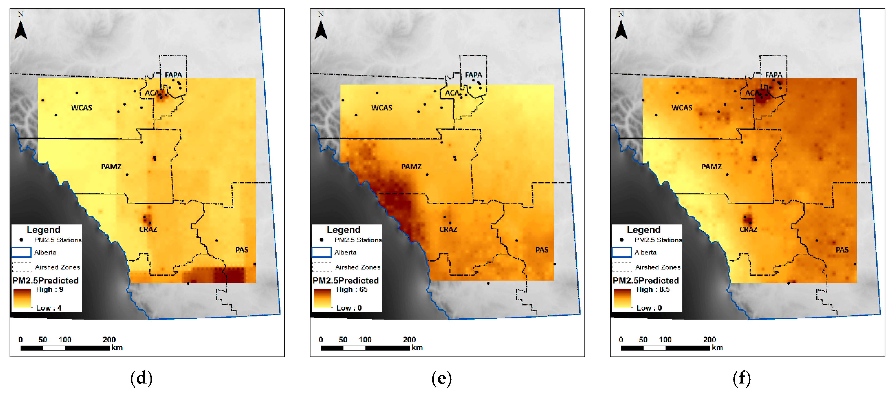
PM_2.5 Predictive PM_2.5 Maps

To extend the estimation of PM_2.5 to the entire study area, a 10 by 10 km grid was overlaid to the study area. First, the value of the model’s variables at the center of each grid cell was extracted, and then, by using the developed models for each sub-period (shown in Table 4 and Equations (2)–(4)), the PM_2.5 levels were calculated at each grid center. An IDW interpolation technique was applied to interpolate the PM_2.5 level between grid centers. The predictive maps are shown in Figure 3.

4. Discussion

4.1. Relation between AOD and PM_2.5 Based on Different Smoke Levels

The results of both AOD and AOD-LUR, for all periods, indicate that with lower level of PM_2.5 concentration, the predictive ability of AOD in the models decreased. Studies have shown that satellite AOD is well suited for detecting large changes in aerosol content [36], which can explain the higher performance of the during-fire models compared to pre- and post-fire models. The increased level of PM_2.5 concentration increases the correlation between AOD and PM_2.5, leading to a better model performance. The graph in Figure 2 demonstrates the difference in PM_2.5 concentration in the during-fire period compared to the other two periods, and it can be seen from the graph that there is also a small peak in the pre-fire period between 11 and 15 August. It is clear from both uni- and multivariate models that the AOD models improved when the smoke from the wildfire drifted over the study area, leading to a high level of PM_2.5. However, both for the pre- and post-fire periods, when the levels of PM_2.5 were fairly low, the model performance decreased due to the lower correlation between AOD and PM_2.5 (mean PM_2.5 = 4.2 µg/m³ compared to 6.2 µg/m³ and 19.5 µg/m³ for pre- and during-fire periods).

The main difference between the post-fire model verses pre- and during-fire models was that the AOD showed little correlation with PM_2.5 level and it was not significant either in the univariate model or in the integrated AOD-LUR model. The relatively weak results obtained by the AOD-model in the post-fire period, compared to the pre- and during-fire period, may be due to uncertainties in MODIS AOD data, such as cloudy days. In southern Alberta, the month of September experiences gradually increasing cloud cover. For example, the percentage of time that the sky is mostly cloudy increases from 42% to 47% in Calgary, 37% to 44% in Lethbridge, 44% to 48% in Red Deer between 1 September and 30 September [68] . The increasing number of cloudy days in September (the post-fire period) have affected the performance of the model using AOD image due to the uncertainty in the AOD data.

4.2. Selected Predictor Variables

Although all three sub-periods used the same study area with almost the same AQ monitoring stations for developing the multivariate models, each final model included a different set of variables. The variable selection of the integrated AOD-LUR models highlights one key finding of this study: The predictors of PM_2.5 vary even over a short period of time (two months), as a function of the presence/absence of wildfire smoke. For example, for the pre-fire period, the variable selection methods identified two variables: AOD, and road length on a 1000-m buffer. By adding the road length variable to the AOD-based regression, the model’s R² value increased from 0.29 to 0.50, emphasizing the major impact of traffic emissions, especially in urban areas. The predictive ability of the during-fire model using both AOD and AOD-LUR model was greater than pre- and post-fire models.

4.3 Relation between PM_2.5 and NDVI

The negative correlation of −0.60% between NDVI and PM_2.5 in the during-fire model (Table 4) indicates that with an increased amount of vegetation, that is, plants and trees around the ground monitoring stations, the level of PM_2.5 decreases. Trees have the ability to reduce significant amounts of ambient air pollutants, by primary absorbing pollution components via leaf stomata and plant surface, and also by intercepting airborne particles [56]. Most of the intercepted particles are retained on the plant surface [56]. The significantly higher coefficient of NDVI in the AOD-LUR model (in absolute value) than the coefficients of the other variables may also indicate the essential role of plants and vegetation in controlling wildfire-related PM_2.5 level. Few studies have applied the greenness index as a predictor in PM_2.5 modeling. However, the role of vegetation and plants in reducing air pollution during the fire events has not been assessed yet.

4.4. Relation between PM_2.5 and Prevailing Wind Speed

The maps in Figure 3 show the spatial pattern of PM_2.5 levels in the three sub-period and displays a temporal pattern over the study period. This pattern appears to be associated with the source of fire (south-west of Alberta) and prevailing wind direction that in the summer is from west to east in most of Alberta. In the first period, when most of the study area’s monitoring stations showed standard levels of PM_2.5, the predicted map shows an elevated level of PM_2.5 in a small portion of southern Alberta. In the rest of the study area, the road length variable is associated with the PM_2.5 concentration, and, as it can be seen in the predictive map, the level of PM_2.5 inside the cities is higher than the level of PM_2.5 in areas further out, where the road network is sparse.

During the fire period, the movement of the fire smoke to the interior portion of the study area is clear: The north and northeast portions of the study area, that are farther from the source of fire are still clean compared to its south and south-west portions.

The PM_2.5 pattern in September, just after the fire, shows higher PM_2.5 concentration in east and northeast areas and lower in west and southwest areas. Even though we used coarse resolution AOD images, the correlation of AOD and PM_2.5 in two of the three sub-periods exhibited the highest value among all predictors, and it was a one of the most significant predictors of PM_2.5.

Wind speed was not significant in any of the models, but it is interesting to note that the correlation between PM_2.5 concentration and wind speed during the fire had opposite signs, in comparison to pre- and post-fire period (correlation between wind speed (at during-fire period) and PM_2.5 = 0.60 and correlation between wind speed-pre/post-fire and PM_2.5 = −0.15). The strong positive correlation between wind speed and PM_2.5 concentrations in the during-fire period is due to the prevailing wind direction in southern Alberta. As the prevailing wind direction during the summer is from west to east in most of Alberta, and the fire was located south-west of Alberta, the higher wind during the fire would result in higher PM_2.5 concentration. Conversely, in the pre-and post-fire periods the wind helps to scatter the pollution and there was a negative correlation between wind speed and PM_2.5, and low winds allow PM_2.5 levels to rise [69].

4.5. Spatial Autocorrelation between AQ Measurements

PM_2.5 over AQ stations did not exhibit significant spatial autocorrelation, nor did any of the model residuals. This result is consistent with the known characteristics of PM_2.5: A regional pollutant, which tends to exhibit little spatial variation. However, as spatial autocorrelation is an indication of self-similarity over short distances, it would be a reasonable expectation during a wildfire event. Non-significant spatial autocorrelation may be related to a smooth pollution pattern, driven by wind and elevation, but it could also be a function of the relatively large distance between the AQ stations. Owing to non-significant spatial autocorrelation in model residuals, reliable result estimates can be obtained from simple linear (OLS) models.

4.6. Validating the Models by Leve-One-Out Cross Validation Procedure

As we mentioned before, the limitation of the present study was the limited number of AQ stations. Therefore, it was not possible to have a separate dataset to validate the models. So, the models’ performance was evaluated using a leave-one-out cross validation method. Comparing R² and adjusted R² of the full training dataset model with the CV-R² shows small decrease in most of the models (between 5% and 10%), which may indicate the reliability of the performance of the models and the generalization ability of the models for a new data set.

Further support for the usefulness of most of the developed models, especially multivariate models, is that both RMSE and CV-RMSE were low compared to the range in measured PM_2.5 concentrations (Table 2 and Table 4).

We can then say that the validation results indicate that the calibrated proposed models, especially during-fire models could be used to estimate PM_2.5 for other fire events in Southern Alberta.

4.7. Application of Integrated AOD-LUR Models in Rural Area

Most studies focus on urban areas due to the lack of AQ monitors in rural area as well as to higher air pollution in urban areas resulting from human activities. The present study estimated wildfire-related PM_2.5, as it relates to source of fire, as opposed to fossil fuel emissions in both urban and rural areas. The results demonstrate that the use of satellite imagery and other land-use (LU) variables can produce a model that might be useful in areas that suffer from the scarcity of AQ monitors. Our study area, southern Alberta, despite including eight airshed zones, only has 24 AQ monitors that measured PM_2.5, most of them located in urban areas. By incorporating MODIS AOD and LU variables, we developed three models for three periods that estimated PM_2.5 in both urban and rural area. Even though the sparseness of AQ stations remains problematic, the proposed models yield preliminary estimates of air pollution at relatively fine spatial resolution in rural areas. Hence, epidemiological studies could use our model results to assess PM_2.5 effect on human health in both rural and urban areas. Further, these predictive models are applicable to other wildfire events, and could help health authorities estimate the spatial and temporal pattern of smoke, with relative accuracy, in major wildfire events.

5. Conclusions

In summary, we proposed a method applicable globally and regionally, which integrates the use of MODIS AOD data into LUR models to identify smoke (particulate matter) concentration. Univariate AOD and multivariate AOD-LUR models were developed to estimate the level of PM_2.5 concentration in three different sub-periods: Pre-, during-, and post-fire. The AOD model performed substantially better when combined with other covariates during the fire period, compared to the univariate AOD model. The predictors in each period varied as a function of the sources of PM_2.5. The three different sub-periods exhibited very large differences in PM_2.5 concentration levels, as well as in the source of PM_2.5. For this reason, separate models were developed for each sub-period. The three univariate models differ from each other in the coefficients, goodness of fit, and other regression diagnostics. The integrated multivariate AOD-LUR models further differ from each other in that each model contains its own set of predictors, with their own associated coefficients.

In addition, our model estimated PM_2.5 concentration at finer spatial scale compared to ground-based measurements available from Alberta airshed zones, which exhibit a sparse distribution of AQ monitors, far from sufficient for public health and epidemiological studies. The spatial and temporal estimates yielded by these models are particularly useful in rural areas, where such estimates are rarely available. Furthermore, the model estimates can aid health authorities predict wildfire smoke exposure at fine spatial and temporal scale, allowing them to better plan for wildfire events, which are likely to increase in frequency and intensity as climate changes.

The result of this study could also be used in epidemiological studies to assess health effects of smoke-related particulate matter during wildfire events, in contrast with those of particulate matter pollution originating from other sources. The results improved the spatial accuracy and reliability of the estimation of wildfire-related PM_2.5, enabling epidemiological studies to assess the association between PM_2.5 and smoke-related health effects during wildfire episodes. To this end, it is essential for epidemiological studies to distinguish between wildfire-related PM_2.5 and PM_2.5 originating from other sources [15]. An important contribution of this paper is the comparison of PM_2.5 level during-fire events, in contrast to pre-fire and post-fire periods. Distance from the wildfire is a significant predictor of PM_2.5 during the fire event, in contrast with the pre- and post-fire period, when the main predictors are transportation and industrial activities. Therefore, by estimated pre and post PM_2.5 maps, the PM_2.5 related health effects before and after fire periods can be evaluated and compared with smoke-related disease.

Further directions of enquiry include the calibration of the proposed models to estimate PM_2.5 for other fire events, in southern Alberta and other regions. We plan to experiment with the use of different satellite AOD data, to obtain even greater spatial accuracy, through the use of finer resolution AOD, which will allow for filling the current MODIS AOD gaps.

References

1. Urbanski, S.P.; Hao, W.M.; Baker, S. Chapter 4 Chemical Composition of Wildland Fire Emissions. Dev. Environ. Sci. 2008, 8, 79–107. [Google Scholar] [CrossRef]
2. California Air Resources Board, Health and the California Department of Public Wildfire Smoke A Guide for Public Health Officials, California. 2011. Available online: https://oehha.ca.gov/media/wildfiresmoke2016.pdf (accessed on 22 April 2018).
3. Reid, C.E.; Jerrett, M.; Tager, I.B.; Petersen, M.L.; Mann, J.K.; Balmes, J.R. Differential respiratory health effects from the 2008 northern California wildfires: A spatiotemporal approach. Environ. Res. 2016, 150, 227–235. [Google Scholar] [CrossRef] [PubMed] [Green Version]
4. Johnston, F.H.; Henderson, S.B.; Chen, Y.; Randerson, J.T.; Marlier, M.; DeFries, R.S.; Kinney, P.; Bowman, D.M.J.S.; Brauer, M. Estimated global mortality attributable to smoke from landscape fires. Environ. Health Perspect. 2012, 120, 695–701. [Google Scholar] [CrossRef] [PubMed]
5. Kollanus, V.; Tiittanen, P.; Niemi, J.V.; Lanki, T. Effects of long-range transported air pollution from vegetation fires on daily mortality and hospital admissions in the Helsinki metropolitan area, Finland. Environ. Res. 2016, 151, 351–358. [Google Scholar] [CrossRef] [PubMed]
6. Alberta Health Services. Wildfire Smoke and Your Health. 2018. Available online: https://myhealth.alberta.ca/Alberta/AlbertaDocuments/wildfire-smoke-and-your-health.pdf (accessed on 5 July 2018).
7. Finlay, S.E.; Moffat, A.; Gazzard, R.; Baker, D.; Murray, V. Health impacts of wildfires. PLoS Curr. 2012, 1–28. [Google Scholar] [CrossRef] [PubMed]
8. World Health Organization. Health Effects of Particulate Matter: Policy Implications for Countries in Eastern Europe, Caucasus and Central Asia. 2013. Available online: http://www.euro.who.int/en/health-topics/environment-and-health/air-quality/publications/2013/health-effects-of-particulate-matter.-policy-implications-for-countries-in-eastern-europe,-caucasus-and-central-asia-2013 (accessed on 10 May 2018).
9. Gupta, P.; Christopher, S.A.; Wang, J.; Gehrig, R.; Lee, Y.; Kumar, N. Satellite remote sensing of particulate matter and air quality assessment over global cities. Atmos. Environ. 2006, 40, 5880–5892. [Google Scholar] [CrossRef]
10. Natural Resources Canada. Indicator: Forest fires. Available online: https://www.nrcan.gc.ca/forests/report/disturbance/16392 (accessed on 17 June 2018).
11. NASA. Pacific Northwest Wildfires Severe in Intensity. Available online: https://www.nasa.gov/image-feature/goddard/pacific-northwest-wildfires-severe-in-intensity (accessed on 22 May 2018).
12. Chen, L.; Verrall, K.; Tong, S. Air particulate pollution due to bushfires and respiratory hospital admissions in Brisbane, Australia. Int. J. Environ. Health Res. 2006, 16, 181–191. [Google Scholar] [CrossRef] [PubMed] [Green Version]
13. Morgan, G.; Sheppeard, V.; Khalaj, B.; Ayyar, A.; Lincoln, D.; Jalaludin, B.; Beard, J.; Corbett, S.; Lumley, T. Effects of bushfire smoke on daily mortality and hospital admissions in Sydney, Australia. Epidemiology 2010, 21, 47–55. [Google Scholar] [CrossRef] [PubMed]
14. Liousse, C.; Guillaume, B.; Grégoire, J.M.; Mallet, M.; Galy, C.; Pont, V.; Akpo, A.; Bedou, M.; Castéra, P.; Dungall, L.; et al. Updated African biomass burning emission inventories in the framework of the AMMA-IDAF program, with an evaluation of combustion aerosols. Atmos. Chem. Phys. 2010, 10, 9631–9646. [Google Scholar] [CrossRef] [Green Version]
15. Youssouf, H.; Liousse, C.; Roblou, L.; Assamoi, E.M.; Salonen, R.O.; Maesano, C.; Banerjee, S.; Annesi-Maesano, I. Quantifying wildfires exposure for investigating health-related effects. Atmos. Environ. 2014, 97, 239–251. [Google Scholar] [CrossRef]
16. De Hoogh, K.; Gulliver, J.; van Donkelaar, A.; Martin, R.V.; Marshall, J.D.; Bechle, M.J.; Cesaroni, G.; Pradas, M.C.; Dedele, A.; Eeftens, M.; et al. Development of West-European PM2.5 and NO2 land use regression models incorporating satellite-derived and chemical transport modelling data. Environ. Res. 2016, 151, 1–10. [Google Scholar] [CrossRef] [PubMed]
17. Eeftens, M.; Beelen, R.; de Hoogh, K.; Bellander, T.; Cesaroni, G.; Cirach, M.; Declercq, C.; Dedele, A.; Dons, E.; de Nazelle, A.; et al. Development of land use regression models for PM2.5, PM2.5 absorbance, PM10 and PMcoarse in 20 European study areas; Results of the ESCAPE project. Environ. Sci. Technol. 2012, 46, 11195–11205. [Google Scholar] [CrossRef] [PubMed]
18. Zhai, L.; Zou, B.; Fang, X.; Luo, Y.; Wan, N.; Li, S. Land use regression modeling of PM2.5 concentrations at optimized spatial scales. Atmosphere 2017, 8, 1–15. [Google Scholar] [CrossRef]
19. Habermann, M.; Billger, M.; Haeger-Eugensson, M. Land use regression as method to model air pollution. Previous results for Gothenburg/Sweden. Procedia Eng. 2015, 115, 21–28. [Google Scholar] [CrossRef]
20. Bertazzon, S.; Johnson, M.; Eccles, K.; Kaplan, G.G. Accounting for spatial effects in land use regression for urban air pollution modeling. Spat. Spatiotemporal. Epidemiol. 2015, 14, 9–21. [Google Scholar] [CrossRef] [PubMed]
21. Li, S.; Joseph, E.; Min, Q. Remote sensing of ground-level PM2.5 combining AOD and backscattering profile. Remote Sens. Environ. 2016, 183, 120–128. [Google Scholar] [CrossRef]
22. Wang, C.; Liu, Q.; Ying, N.; Wang, X.; Ma, J. Air quality evaluation on an urban scale based on MODIS satellite images. Atmos. Res. 2013, 132, 22–34. [Google Scholar] [CrossRef]
23. Van Donkelaar, A.; Martin, R.V.; Park, R.J. Estimating ground-level PM2.5 using aerosol optical depth determined from satellite remote sensing. J. Geophys. Res. Atmos. 2006, 111, 1–10. [Google Scholar] [CrossRef]
24. Christopher, S.A.; Gupta, P. Satellite Remote Sensing of Particulate Matter Air Quality: The Cloud-Cover Problem. J. Air Waste Manag. 2010, 60, 596–602. [Google Scholar] [CrossRef] [Green Version]
25. Hodzic, A.; Madronich, S.; Bonn, B.; Massie, S.; Menut, L.; Wiedinmyer, C. Wildfire particulate matter in Europe during summer 2003: Meso-scale modeling of smoke emissions, transport and radiative effects. Atmos. Chem. Phys. 2007, 7, 4043–4064. [Google Scholar] [CrossRef] [Green Version]
26. Kloog, I.; Koutrakis, P.; Coull, B.A.; Lee, H.J.; Schwartz, J. Assessing temporally and spatially resolved PM2.5 exposures for epidemiological studies using satellite aerosol optical depth measurements. Atmos. Environ. 2011, 45, 6267–6275. [Google Scholar] [CrossRef]
27. Chudnovsky, A.A.; Lee, H.J.; Kostinski, A.; Kotlov, T.; Koutrakis, P. Prediction of daily fine particulate matter concentrations using aerosol optical depth retrievals from the Geostationary Operational Environmental Satellite (GOES). J. Air Waste Manag. Assoc. 2012, 62, 1022–1031. [Google Scholar] [CrossRef] [PubMed] [Green Version]
28. Tao, J.H.; Zhang, M.G.; Chen, L.F.; Wang, Z.F.; Su, L.; Ge, C.; Han, X.; Zou, M.M. A method to estimate concentrations of surface-level particulate matter using satellite-based aerosol optical thickness. Sci. China Earth Sci. 2013, 56, 1422–1433. [Google Scholar] [CrossRef]
29. Liu, Y.; Franklin, M.; Kahn, R.; Koutrakis, P. Using aerosol optical thickness to predict ground-level PM2.5 concentrations in the St. Louis area: A comparison between MISR and MODIS. Remote Sens. Environ. 2007, 107, 33–44. [Google Scholar] [CrossRef]
30. Chu, D.A.; Szykman, J.; Kondragunta, S. Analysis of the relationship between MODIS aerosol optical depth and PM2.5 in the summertime US. In Proc. SPIE; SPIE Digital Library: San Diego, CA, USA, 2006; Volume 6299, Available online: https://doi.org/10.1117/12.678841 (accessed on 10 May 2018).
31. Anselin, L.; Le Gallo, J. Interpolation of Air Quality Measures in Hedonic House Price Models: Spatial Aspects. Spat. Econ. Anal. 2006, 1, 31–52. [Google Scholar] [CrossRef]
32. Mercer, L.D.; Szpiro, A.A.; Sheppard, L.; Lindström, J.; Adar, S.D.; Allen, R.W.; Avol, E.L.; Oron, A.P.; Larson, T.; Liu, L.J.S.; et al. Comparing universal kriging and land-use regression for predicting concentrations of gaseous oxides of nitrogen (NOx) for the Multi-Ethnic Study of Atherosclerosis and Air Pollution (MESA Air). Atmos. Environ. 2011, 45, 4412–4420. [Google Scholar] [CrossRef] [PubMed]
33. Jerrett, M.; Arain, A.; Kanaroglou, P.; Beckerman, B.; Potoglou, D.; Sahsuvaroglu, T.; Morrison, J.; Giovis, C. A review and evaluation of intraurban air pollution exposure models. J. Expo. Sci. Env. Epid. 2005, 15, 185–204. [Google Scholar] [CrossRef] [PubMed]
34. Hu, Z. Spatial analysis of MODIS aerosol optical depth, PM2.5, and chronic coronary heart disease. Int. J. Health Geogr. 2009, 8, 1–10. [Google Scholar] [CrossRef] [PubMed]
35. Ma, Z.; Hu, X.; Huang, L.; Bi, J.; Liu, Y. Estimating ground-level PM2.5 in China using satellite remote sensing. Environ. Sci. Technol. 2014, 48, 7436–7444. [Google Scholar] [CrossRef] [PubMed]
36. Lassman, W.; Ford, B.; Gan, R.W.; Pfister, G.; Magzamen, S.; Fischer, E.V.; Pierce, J.R. Spatial and temporal estimates of population exposure to wildfire smoke during the Washington state 2012 wildfire season using blended model, satellite, and in situ data. GeoHealth 2017, 1, 106–121. [Google Scholar] [CrossRef] [Green Version]
37. Lin, C.; Li, Y.; Yuan, Z.; Lau, A.K.H.; Li, C.; Fung, J.C.H. Using satellite remote sensing data to estimate the high-resolution distribution of ground-level PM2.5. Remote Sens. Environ. 2015, 156, 117–128. [Google Scholar] [CrossRef]
38. Van Donkelaar, A.; Martin, R.V.; Spurr, R.J.D.; Burnett, R.T. High-Resolution Satellite-Derived PM2.5 from Optimal Estimation and Geographically Weighted Regression over North America. Environ. Sci. Technol. 2015, 49, 10482–10491. [Google Scholar] [CrossRef] [PubMed]
39. Kloog, I.; Chudnovsky, A.A.; Just, A.C.; Nordio, F.; Koutrakis, P.; Coull, B.A.; Lyapustin, A.; Wang, Y.; Schwartz, J. A new hybrid spatio-temporal model for estimating daily multi-year PM2.5 concentrations across northeastern USA using high resolution aerosol optical depth data. Atmos. Environ. 2014, 95, 581–590. [Google Scholar] [CrossRef] [PubMed]
40. Wang, J. Intercomparison between satellite-derived aerosol optical thickness and PM2.5 mass: Implications for air quality studies. Geophys. Res. Lett. 2003, 30, 2095. [Google Scholar] [CrossRef]
41. Chu, D.A.; Kaufman, Y.J.; Zibordi, G.; Chern, J.D.; Mao, J.; Li, C.; Holben, B.N. Global monitoring of air pollution over land from the Earth Observing System-Terra Moderate Resolution Imaging Spectroradiometer (MODIS). J. Geophys. Res. Atmos. 2003, 108, 1–18. [Google Scholar] [CrossRef]
42. Kacenelenbogen, M.; Léon, J.F.; Chiapello, I.; Tanré, D. Characterization of aerosol pollution events in France using ground-based and POLDER-2 satellite data. Atmos. Chem. Phys. 2006, 6, 4843–4849. [Google Scholar] [CrossRef] [Green Version]
43. Pm, G.; Paciorek, C.J.; Moreno-Macias, H. Spatio-temporal Associations Between GOES Aerosol Optical Depth Retrievals and Ground-Level PM2.5. Environ. Sci Technol. 2008, 42, 5800–5806. [Google Scholar] [CrossRef]
44. Chu, Y.; Liu, Y.; Li, X.; Liu, Z.; Lu, H.; Lu, Y.; Mao, Z.; Chen, X.; Li, N.; Ren, M.; et al. A review on predicting ground PM2.5 concentration using satellite aerosol optical depth. Atmosphere 2016, 7, 1–25. [Google Scholar] [CrossRef]
45. Chudnovsky, A.A.; Koutrakis, P.; Kloog, I.; Melly, S.; Nordio, F.; Lyapustin, A.; Wang, Y.; Schwartz, J. Fine particulate matter predictions using high resolution Aerosol Optical Depth (AOD) retrievals. Atmos. Environ. 2014, 89, 189–198. [Google Scholar] [CrossRef]
46. Yang, X.; Zheng, Y.; Geng, G.; Liu, H.; Man, H.; Lv, Z.; He, K.; de Hoogh, K. Development of PM2.5 and NO2 models in a LUR framework incorporating satellite remote sensing and air quality model data in Pearl River Delta region, China. Environ. Pollut. 2017, 226, 143–153. [Google Scholar] [CrossRef] [PubMed]
47. Environment and Climate Change Canada. Canadian Environmental Sustainability Indicators: Air pollutant emissions. 2017. Available online: https://www.canada.ca/en/environment-climate-change/services/environmental-indicators/air-pollutant-emissions.html (accessed on 12 June 2018).
48. Van Donkelaar, A.; Martin, R.V.; Brauer, M.; Hsu, N.C.; Kahn, R.A.; Levy, R.C.; Lyapustin, A.; Sayer, A.M.; Winker, D.M. Global Estimates of Fine Particulate Matter using a Combined Geophysical-Statistical Method with Information from Satellites, Models, and Monitors. Environ. Sci. Technol. 2016, 50, 3762–3772. [Google Scholar] [CrossRef] [PubMed]
49. Zheng, Y.; Zhang, Q.; Liu, Y.; Geng, G.; He, K. Estimating ground-level PM2.5 concentrations over three megalopolises in China using satellite-derived aerosol optical depth measurements. Atmos. Environ. 2016, 124, 232–242. [Google Scholar] [CrossRef]
50. Van Donkelaar, A.; Martin, R.V.; Brauer, M.; Kahn, R.; Levy, R.; Verduzco, C.; Villeneuve, P.J. Global estimates of ambient fine particulate matter concentrations from satellite-based aerosol optical depth: Development and application. Environ. Health Perspect. 2010, 118, 847–855. [Google Scholar] [CrossRef] [PubMed]
51. Gupta, P.; Christopher, S.A. Seven year particulate matter air quality assessment from surface and satellite measurements. Atmos. Chem. Phys. 2008, 8, 3311–3324. [Google Scholar] [CrossRef] [Green Version]
52. Hutchison, K.D.; Faruqui, S.J.; Smith, S. Improving correlations between MODIS aerosol optical thickness and ground-based PM2.5 observations through 3D spatial analyses. Atmos. Environ. 2008, 42, 530–543. [Google Scholar] [CrossRef]
53. Lee, H.J.; Coull, B.A.; Bell, M.L.; Koutrakis, P. Use of satellite-based aerosol optical depth and spatial clustering to predict ambient PM2.5 concentrations. Environ. Res. 2012, 118, 8–15. [Google Scholar] [CrossRef] [PubMed]
54. Chudnovsky, A.; Lyapustin, A.; Wang, Y.; Schwartz, J.; Koutrakis, P. Analyses of high resolution aerosol data from MODIS satellite: A MAIAC retrieval, southern New England, US. 2013, 87951E. [Google Scholar] [CrossRef]
55. Montagne, D.R.; Hoek, G.; Klompmaker, J.O.; Wang, M.; Meliefste, K.; Brunekreef, B. Land Use Regression Models for Ultrafine Particles and Black Carbon Based on Short-Term Monitoring Predict Past Spatial Variation. Environ. Sci. Technol. 2015, 49, 8712–8720. [Google Scholar] [CrossRef] [PubMed]
56. Nowak, D.J.; Crane, D.E.; Stevens, J.C. Air pollution removal by urban trees and shrubs in the United States. Urban For. Urban Green. 2006, 4, 115–123. [Google Scholar] [CrossRef] [Green Version]
57. Wu, C.D.; Chen, Y.C.; Pan, W.C.; Zeng, Y.T.; Chen, M.J.; Guo, Y.L.; Lung, S.C.C. Land-use regression with long-term satellite-based greenness index and culture-specific sources to model PM2.5 spatial-temporal variability. Environ. Pollut. 2017, 224, 148–157. [Google Scholar] [CrossRef] [PubMed]
58. Wu, C.D.; McNeely, E.; Cedeño-Laurent, J.G.; Pan, W.C.; Adamkiewicz, G.; Dominici, F.; Lung, S.C.C.; Su, H.J.; Spengler, J.D. Linking student performance in Massachusetts elementary schools with the “greenness” of school surroundings using remote sensing. PLoS ONE 2014, 9, 1–9. [Google Scholar] [CrossRef] [PubMed] [Green Version]
59. Lee, M.; Kloog, I.; Chudnovsky, A.; Lyapustin, A.; Wang, Y.; Melly, S.; Coull, B.; Koutrakis, P.; Schwartz, J. Spatiotemporal prediction of fine particulate matter using high resolution satellite images in the southeastern U.S. 2003–2011. J. Expo. Sci. Environ. Epidemiol. 2016, 26, 377–384. [Google Scholar] [CrossRef] [PubMed]
60. Sampson, P.D.; Richards, M.; Szpiro, A.A.; Bergen, S.; Sheppard, L.; Larson, T.V.; Kaufman, J.D. A regionalized national universal kriging model using Partial Least Squares regression for estimating annual PM2.5 concentrations in epidemiology. Atmos. Environ. 2013, 75, 383–392. [Google Scholar] [CrossRef] [PubMed]
61. National Road Network (NRN)—AB, Alberta. Available online: https://open.alberta.ca/opendata/cb1d2fbd-4695-4cac-accd-40db2774f23d (accessed on 11 May 2018).
62. National Pollutant Release Inventory (NPRI). Available online: http://www.ec.gc.ca/inrp-npri/default.asp?lang%BCEn&;n%BC4A577BB9-1 (accessed on 12 July 2018).
63. DMTI. The Gold Standard Canada’s Most Complete and Accurate Mapping Data. Available online: https://www.dmtispatial.com/ (accessed on 1 July 2018).
64. Acker, J.G.; Leptoukh, G. Online Analysis Enhances Use of NASA Earth Science Data. Eos Trans. Am. Geophys. Union 2007, 88, 14. [Google Scholar] [CrossRef]
65. Getis, A. A history of the concept of spatial autocrrelation: A geographer’s perspective. Geogr. Anal. 2008, 40, 297–309. [Google Scholar] [CrossRef]
66. Anselin, L.; Bera, A.K.; Florax, R.; Yoon, M.J. Simple diagnostic tests for spatial dependence. Reg. Sci. Urban Econ. 1996, 26, 77–104. [Google Scholar] [CrossRef]
67. How Inverse Distance Weighted Interpolation Work. Available online: http://pro.arcgis.com/en/pro-app/help/analysis/geostatistical-analyst/how-inverse-distance-weighted-interpolation-works.htm (accessed on 22 May 2018).
68. Weather Spark The Typical Weather Anywhere on Earth. Available online: https://weatherspark.com/ (accessed on 18 August 2018).
69. Chaloulakou, A.; Kassomenos, P.; Spyrellis, N.; Demokritou, P.; Koutrakis, P. Measurements of PM10 and PM2.5 particle concentrations in Athens, Greece. Atmos. Environ. 2003, 37, 649–660. [Google Scholar] [CrossRef]
Figure 1. Alberta airshed zones (a) (www.albertaairshedscouncil.ca), Distribution of 24 monitoring stations in the Southern Alberta airshed zones used in the present study (b).
Atmosphere 09 00335 g001
Figure 2. Temporal daily variability of PM2.5 level at the 24 stations located at the study area.
Atmosphere 09 00335 g002
Figure 3. The predicted PM2.5 maps over the study area including: Prediction results obtained by models’ coefficient at grid centroid (ac), and interpolated maps between grids (df), for the three periods separately: (a,d) Pre-fire predicted maps, (b,e) during-fire predicted maps, and (c,f) post-fire predicted maps.
Atmosphere 09 00335 g003aAtmosphere 09 00335 g003b