Article

Modelling Wetland Growing Season Rainfall Interception Losses Based on Maximum Canopy Storage Measurements

by
Wojciech Ciężkowski
1,*,
Tomasz Berezowski
2,
Małgorzata Kleniewska
1,
Sylwia Szporak-Wasilewska
3 and
Jarosław Chormański
1
1
Department of Hydraulic Engineering, Faculty of Civil and Environmental Engineering, Warsaw University of Life Sciences, Nowoursynowska 166, 02-787 Warsaw, Poland
2
Faculty of Electronics, Telecommunication and Informatics, Department of Geoinformatics, Gdansk University of Technology, Gabriela Narutowicza 11/12, 80-233 Gdansk, Poland
3
Water Center Laboratory, Faculty of Civil and Environmental Engineering, Warsaw University of Life Sciences, Nowoursynowska 166, 02-787 Warsaw, Poland
*
Author to whom correspondence should be addressed.
Water 2018, 10(1), 41; https://doi.org/10.3390/w10010041
Submission received: 16 November 2017 / Revised: 13 December 2017 / Accepted: 3 January 2018 / Published: 5 January 2018

Abstract

:
This study estimates rainfall interception losses from natural wetland ecosystems based on maximum canopy storage measurements. Rainfall interception losses play an important role in water balance, which is crucial in wetlands, and has not yet been thoroughly studied in relation to this type of ecosystem. Maximum canopy storage was measured using the weight method. Based on these measurements, daily values of interception losses were estimated and then used to calculate long-term interception losses based on precipitation and potential evapotranspiration data for the 1971–2015 period. Depending mainly on the number of days with precipitation, the results show that total interception losses for the growing season as well as monthly interception losses are around 13% of gross rainfall. This value is similar to the values observed for some forests. Hence, interception losses should not be disregarded in hydrologic models of wetlands, especially because data trends in meteorological conditions (mainly number of days with precipitation) show that interception losses will increase in the future if those trends stay the same.

1. Introduction

Rainfall interception is the process where ground surfaces, whether vegetated or sealed because of human construction, catching and retaining water during precipitation [1]. It is of considerable importance in water resource management [2], and in the context of climate change [3]. Phytoelement wetness caused by rainfall interception also plays an important role in many areas such as the control of plant disease [4,5], plant susceptibility to dry and wet acid deposition [6,7], in plant photosynthesis and in plant yield [8,9]. However, the lack of knowledge about rainfall interception means that this process has been disregarded or underestimated in rainfall-runoff analysis [10]. Some models disregard it completely, e.g., the THALES model [11], the Distributed Basin Simulator (DBSIM) model [12], the Representative Elementary Watersheds REW approach [13], and the Topkapi model [14]. Other models simplify interception and lump its value with transpiration: Topmodel [15], European Hydrological modeling System SHE [16], Wetspa [17].
The rain that falls and hits plant surfaces is temporarily retained on the plant surface and, ultimately, either evaporates or makes its way to the ground by throughfall or by flowing down branches and stems [3]. Storage water can be divided into transistor storage (water that drips down immediately), conditional storage (drip out by leaf movements caused, e.g., by wind) and residual storage (water which can be removed only by evaporation) [18]. Residual storage is the most widely examined and it can be represented as: canopy storage [18], water storage capacity [19], canopy rainfall capacity [20] and rainfall interception [1,21].
Most research on rainfall interception by plant canopies has focused on different kinds of trees in different climatic zones, for instances tropical rain forests in Guyana [22], Brazil [23] and eastern Amazonia [24]; tropical montane cloud forest of Guatemala [25]; laurel forest in Canary Island [26]; lowland tropical rainforest in Brunei [27]; boreal forest in Sweden [28]; arid zone pine forest [29]; and deciduous Mediterranean forest in Slovenia [30]. The number of studies on rainfall interception by lower vegetation are inadequate with focuses mainly on: grasslands [19,21,31], drylands [1,20] shrublands [31,32], or croplands [33]. There are two reasons for this. The first is that interception losses from forest are generally greater in absolute volume than those from lower vegetation. However, some studies [31] showed that interception of grasslands can reach approximately 30% of annual rainfall, which is similar to many forests [34]. The second reason is the difficulties in measuring rainfall interception in lower vegetation, especially in natural heterogeneous ecosystems.
Lately, a few studies on rainfall interception have been made in a natural wetland ecosystem in Biebrza Basin (NE Poland). Those studies focused on determining the spatial distribution of interception capacity based on ground truth measurements of maximum canopy storage and ALS (airborne laser scanning) [35], also ground truth data was used with Landsat 7 ETM+ image [36]. There have also been numerous studies conducted on estimation of interception using remote sensing techniques that have focused on forest [37,38], croplands [39] or grasslands [38]. Remote sensing techniques show great potential in estimating the spatial distribution of interception, but ground measurements are mandatory for studies on less well-recognised ecosystems such as wetlands. This study follows increasing interest in interception on wetlands ecosystems and on growing season interception in this area.
Studies on the hydrologic cycle has shown a rising interest in rainfall interception phenomena. Even urban areas, where rainfall interception losses seem to be insignificant, have begun to be investigated for examination of its influence on water balance [40,41]. The main aim of this study is to investigate the influence of hydrological processes and meteorological conditions (precipitation, evapotranspiration, length of growing season, number of days with precipitation) on the amount of intercepted water for the typical land covers in the Biebrza Valley. The second aim is to estimate interception losses for a long time series based on ground measurements of maximum canopy storage. The research focuses only on the growing season due to its length (perennial average 200 days) and the fact that the height and size of analysed plants outside the growing season is negligible. Relation with meteorological conditions together with investigations of the perennial trends of meteorological conditions in year 1971–2015 can show potential influence of climate change on rainfall interception in future. These results might improve hydrological modelling on wetlands and the understanding of wetland ecohydrological processes.

2. Materials and Methods
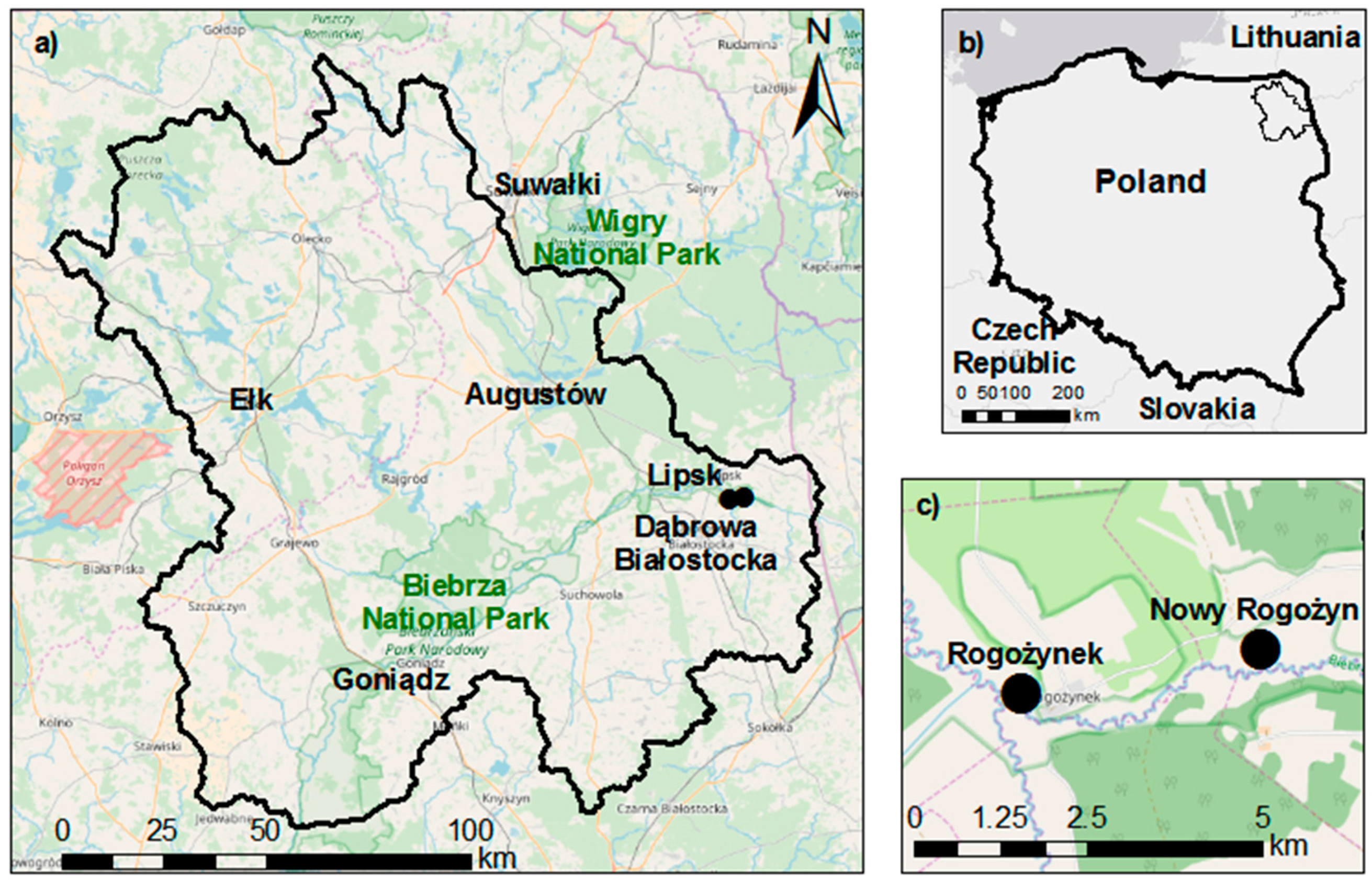
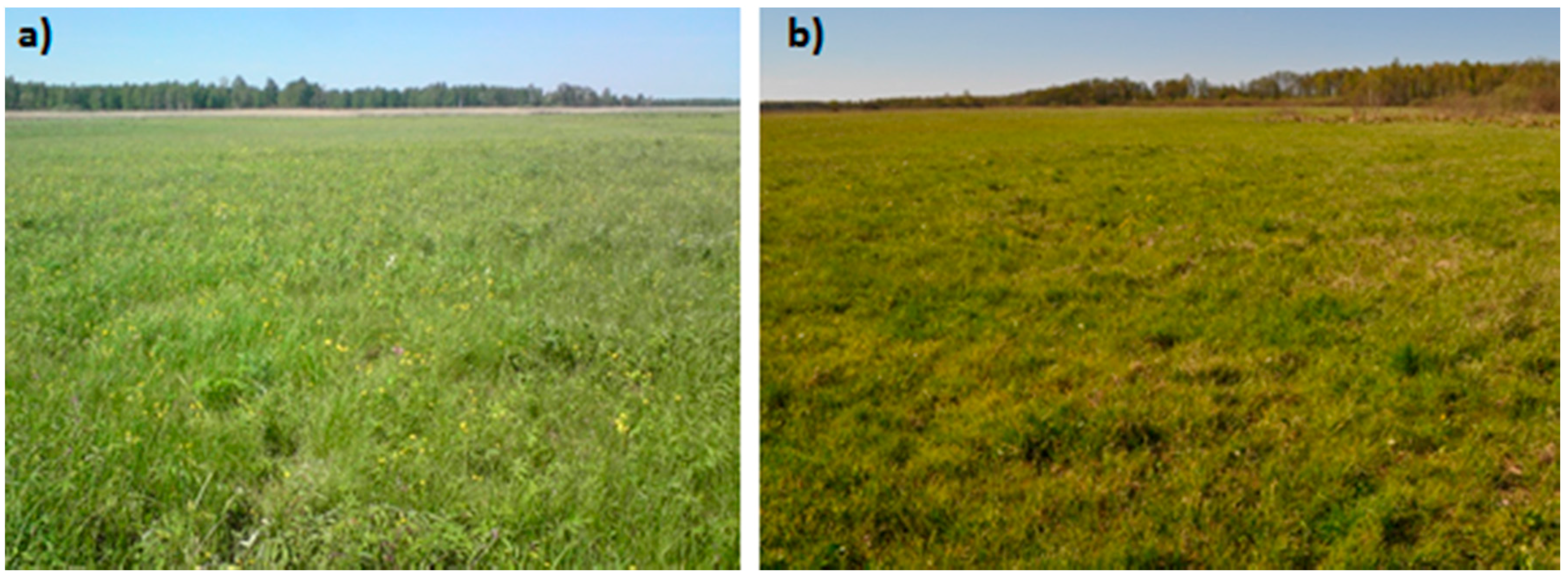
2.1. Study Site

The maximum canopy storage measurements were taken in the upper Biebrza Basin (NE Poland) (Figure 1). The study area is part of a river valley and is dominated by peat soils (mainly peat moss with the exception of areas near the river). The area is inundated due to irregular floods. The dominated plant community is Carici canescentis-Agrostietum caninae, creating a belt of up to 0.6 km wide on both banks along the river. The area is also covered by Caricion lasiocarpae, Molinio-Arrhenatheretea, as well as Phragmitetum communities that grow along the Biebrza River. In sections of the valley abandoned by agriculture, as it is typical of natural river valleys with wetland vegetation, sedges will form in hummock patterns. Research has been conducted on areas covered with phytocenoses of semi-natural plant communities created by a single, extensive, mechanical mowing followed by biomass removal, typically carried out after 1 July, depending on whether soil moisture conditions in the valley are allowing for the entry of field equipment or not. This type of usage is dominant in the study area of the Biebrza valley (Figure 2).
The climate of the Biebrza River Valley is temperate transitional, with evident continental influences. The mean annual air temperature in the basin was 6.6 °C in the years 1961–2000. However, in individual years, the mean values can vary between 4.8 °C and 8.3 °C. The mean annual precipitation ranged from 536 mm to 610 mm, and the mean annual wind speed was 3.8 m∙s−1 [42]. The diverse topography and morphology lead to variations in local and macro-scale climate conditions and high biodiversity, which are the main cause of differences in temperature and humidity in the warm part of the year [43].

2.2. Maximum Canopy Storage Field Measurements

Field measurements focused on determining maximum canopy storage (Imax [mm]) were conducted on two meadows (Figure 1). The two selected meadows (in Nowy Rogożyn and Rogożynek) are mowed one time per year and are representative for the whole Upper Biebrza Basin wetland meadows. Acquired phytosociological relevés from the selected meadows show high variability of vegetation with up to 60 different plant species per meadow.
Measurements are made during three field campaigns in 2014: 26–29 June (1–2 months into the growing season), 28–30 July (peak of growing season) and 4–5 September (plant weeding, 1–2 weeks before the end of the growing season). The dates of field campaigns were chosen to represent changes in plant phenology from the beginning of growth through to the state of full development and plant weeding till the death of the plants. Field campaigns were organized on sunny days in hours when dew was not present. First, in order to characterise plant communities presented in the research area, phytosociological data were collected in relevés. Then, samples were collected by cutting all the above-ground vegetation within a 0.25 m by 0.25 m square. In total, 68 samples were collected, with each sample consisting of 90–250 plants.
All collected plants were immediately transported to a laboratory, where further measurements were conducted in a natural state. Imax was determined by weighting. Imax is calculated as the difference between the freshly collected and the weight of a soaked plant. There are two methods of soaking plants with water: spraying [21,31,32,44] and submerging [1,19,45]. In this study, plants were submerged because it is less ideal with spraying where the droplet size will cause variations [46]. Results obtained by submersion are less dependent on human factors and are more reproducible.
All plants from each square were weighed one by one to an accuracy of 0.01 g using a WPS2100/C scale (RADWAG). Then, to avoid interactions between plants, the plants were submerged in a tank of water one by one. After a few seconds after submersion (to allow the excess water to drip from the leaves), each plant was weighed. The difference between the weight of plants before and after submergence is a factor of Imax in grams per sampling area (0.0625 m2). This value was recalculated into mm of H2O per unit area by dividing the volume of intercepted water (calculated assuming water density equal to 1 g/cm3) by the sampling area.

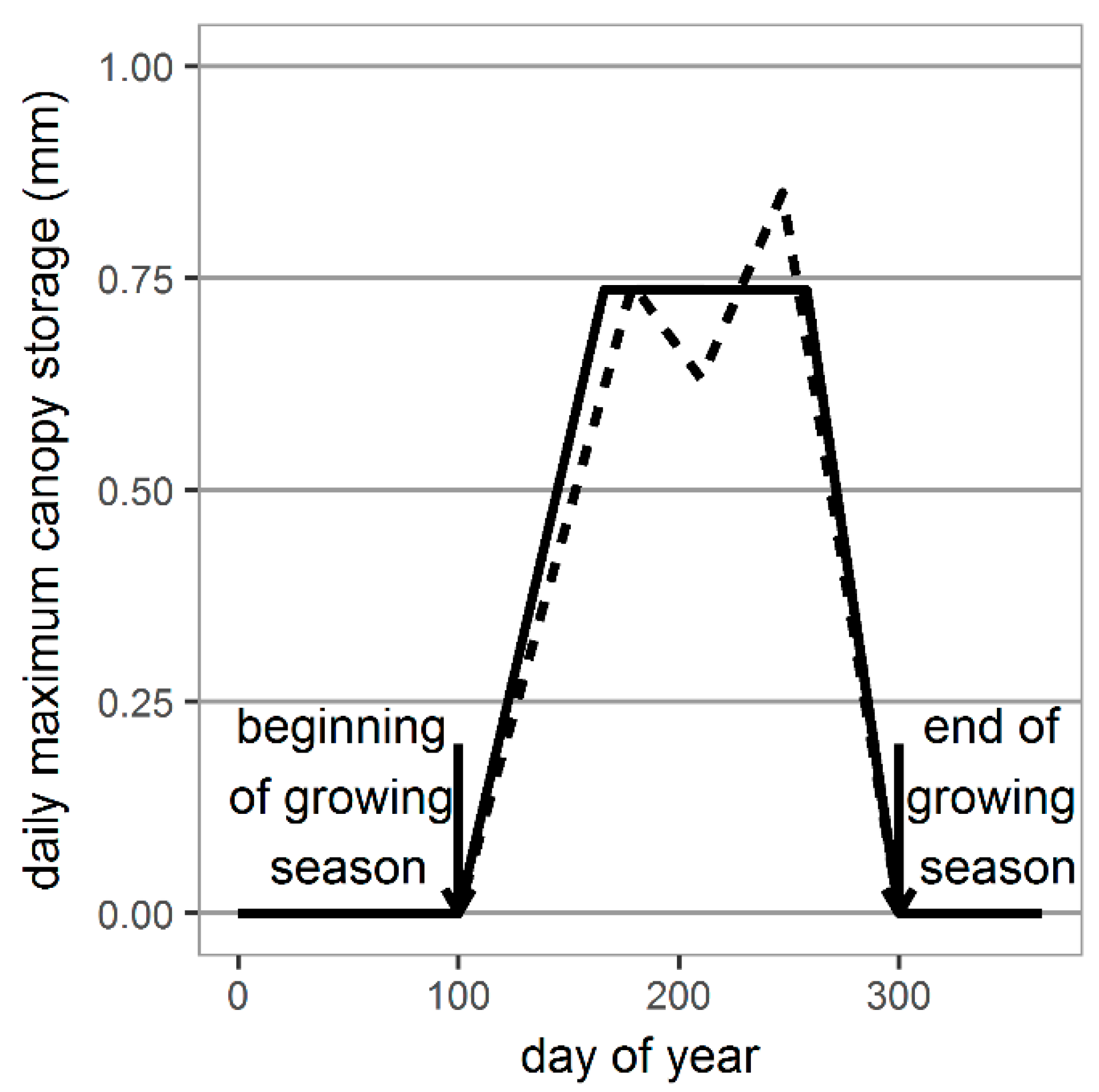
2.3. Generating Daily Values of Maximum Canopy Storage

All measurements of maximum canopy storage were taken in three campaigns during a single growing season, and the means of Imax for the three campaigns were tested for statistical significance in their differences using the ANOVA test. We find the difference not statistically significant with p = 0.141 (Section 3.1). Hence, to obtain perennial daily values of Imax the Monte Carlo method was used. Based on the 2014 measurements (n = 68), 100,000 repetitions of daily unbiased maximum canopy storage samples were generated for the 1971–2015 period. Our measurements distribution was fitted with gamma distribution using the maximum-likelihood estimation method. Gamma distribution was chosen because it is often used to model maximum discharge or precipitation. Maximum canopy storage values can be modelled using gamma distribution. Our tests with other distributions, such as Χ2, lognormal and normal, showed that gamma distribution fits better to the data. The fitted gamma distribution parameters were: shape = 4.704 and rate = 6.386. The fitted distribution is good according to the Kolmogorov–Smirnov test (D = 0.0617, p = 0.95). The generated values were assigned to the mid-day of the 15th days of June, July, August and September. Other values were linearly interpolated assuming that Imax is 0 at the beginning and end of the growing season. Previous research on wetland meadow canopy storage in this area [35,36,45,47] also focused only on the growing season. This is due to the negligible height of sedge communities before and after the growing season in this area. Hence, this study focused on rainfall interception losses in the growing season.
The results of measurements and the example of generated daily maximum canopy storage values are shown in Figure 3. For diurnal calculation, daily values of maximum canopy storage depend on the beginning and end of the growing season, which was calculated based on air temperature (Section 3.2).

2.4. Interception Losses Model

Daily rainfall interception losses (Iday), meaning water that was retained by plants during a given period, were calculated with Equation (1) based on daily precipitation (P), potential evapotranspiration (ET0) (calculated according to [48]) and maximum canopy storage (Imax):
I d a y = { I m a x   i f   P E T 0 > I m a x P E T 0   i f   P E T 0 I m a x .
Calculations of Iday were performed for data from the nearest non-urban meteorological station located in the Biebrza Valley (in Pieńczykówek) for the years 1971 to 2015. Then, it is repeated for all 100,000 simulated values of maximum canopy storage. The meteorological data for Pieńczykowek station were made available by the Institute of Meteorology and Water Management: National Research Institute (IMGW-PIB) in Poland.
This model of rainfall interception is a simple one as there are no well-defined physically-based interception models of wetland vegetation in the study area. The most common physically-based models are Gash [49] and Rutter [34], which were developed for forest ecosystems, and applying them to the ecosystems of our research area was difficult due to the issue of distinguishing certain model parameters (such as trunk storage capacity or free throughfall coefficient, which are technically difficult to define for low vegetation). For this reason, rainfall interception models for grasslands or wetland meadows have not been properly configured. In addition, of the nearly 70 applications we found in the literature, only four were agricultural [3], and these models are difficult to implement due to issues with parametrisation and measurements of rainfall interception. Because of similar reasons, and adding the diversity in natural heterogeneous wetland ecosystems, it is even more difficult to model their rainfall interception.

3. Results

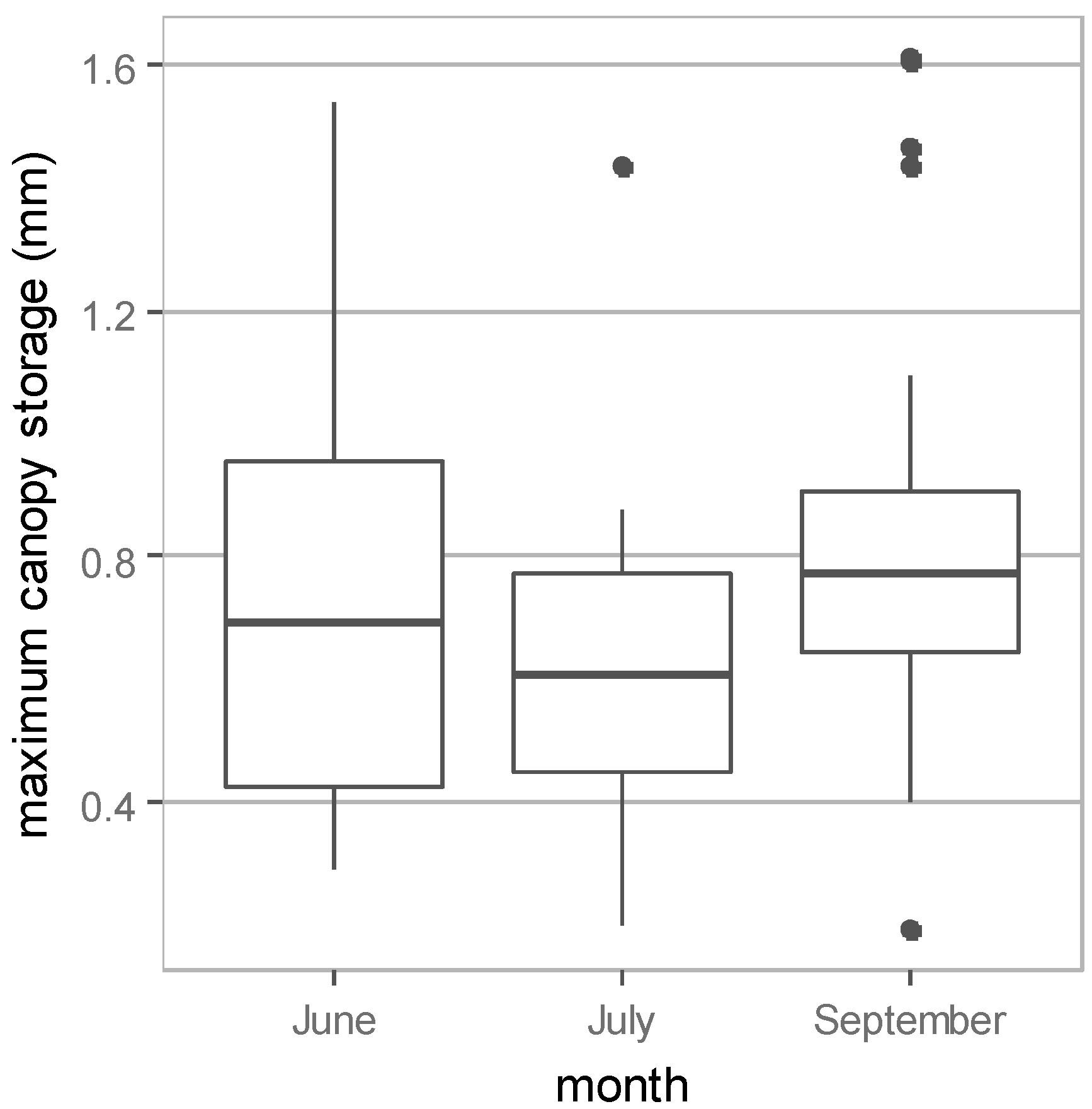
3.1. Field Measurement Results

The results of the three field campaigns are compared in Table 1 and Figure 4. The numbers of samples per campaign varies from 19 in July to 29 in June, but the ANOVA test show no statistically significant relation between the means of maximum canopy storage for these campaigns (p = 0.141). In all months, the standard deviation was about 50% of the mean value, which is caused by high biodiversity (phytosociological relevés were recorded from 24 to 39 different species; in the same sampling areas, the number of species was constant during the growing season). The highest (1.61 mm) and the lowest (0.19 mm) values of Imax were measured in September. Other than high biodiversity that is causing the large variation in values of Imax, plants in September are also going through different stages of their life cycle (some were still growing, while others had already dried out), which is another reason for the big range of observed values in this month. In June and July, all plants are in the same phenological phase. From all campaigns, the mean values of Imax are the same at 0.75 mm.

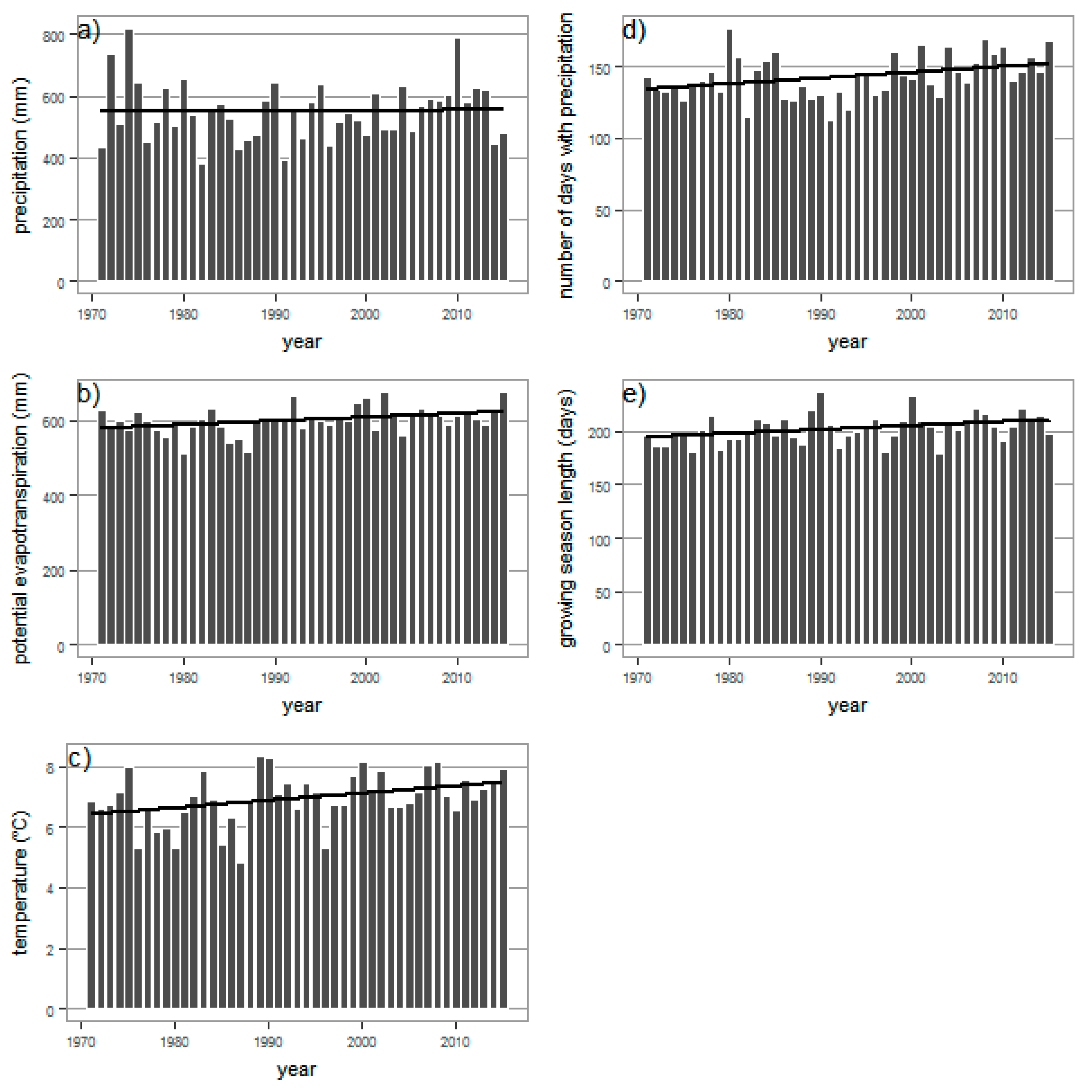
3.2. Meteorological Element Trends, 1971–2015

Based on daily values of air temperature (mean, minimum and maximum), relative humidity and wind speed, potential evapotranspiration was calculated using the Penman–Monteith equation with the FAO (Food and Agriculture Organization of the United Nations) modification [47]. Potential evapotranspiration and daily precipitation are used to investigate perennial trends of precipitation sum, potential evapotranspiration sum, mean temperature and days with precipitation in the whole year and during the growing season. The length of the growing season was also investigated. The growing period in Poland is closely related to the dates on which the +5 °C daily mean air temperature threshold value is permanently crossed. Because the ecological factor that affects the rate of plant life processes is thermal conditions, the duration of the growing period is approximately equal to the thermal growing season [50]. Results for perennial trends are showed in Figure 5. Mean perennial values of meteorological elements and slope of the trend (for whole year and for only growing season) were calculated, and the results are summarized in Table 2. Apart from precipitation and number of days with precipitation in the growing season, all elements show slightly growing trends which are significant (p-value ≤ 0.05). The non-parametric Mann–Kendall trend test was also performed, using the Kendall R package [51]. Results are compared in Table 2 and it shows the same trends as the linear trends.

3.3. Relations between Interception Losses and Meteorological Elements

The daily interception losses calculated in Section 2.4 were used to compute the growing season and monthly sums of interceptions, hereinafter referred to as ‘absolute growing season’ (AIgs) and ‘monthly’ interception (AImonth) expressed in mm. Absolute interception was also divided by growing season or monthly sum of precipitation, which hereinafter are referred to as ‘relative growing season interception’ (RIgs) and ‘relative monthly interception’ losses (RImonth), and are both expressed as percentage of precipitation. Additionally, for both RIgs and RImonth, the relationship with meteorological elements was investigated in the monthly and growing season timescales.

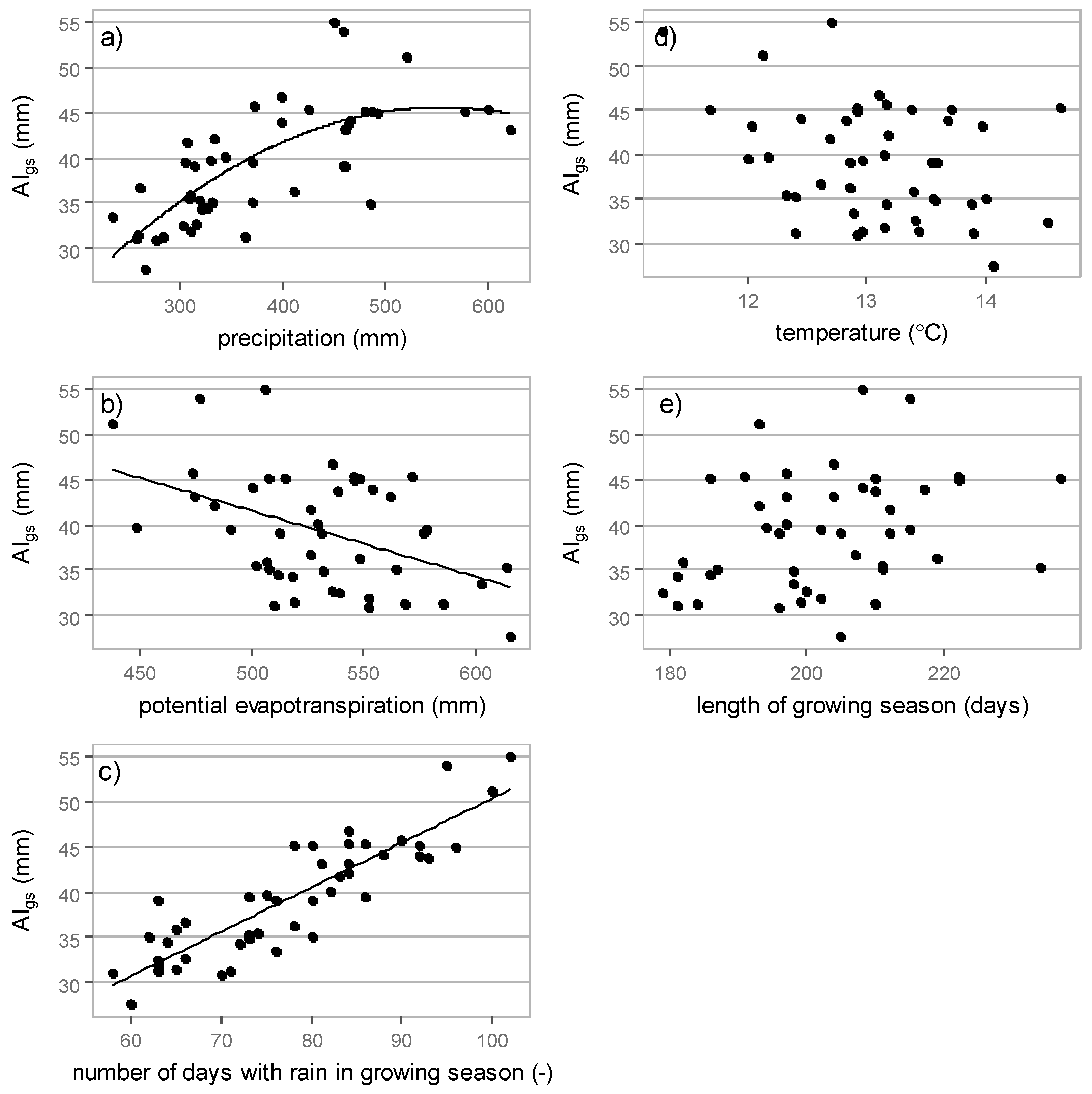
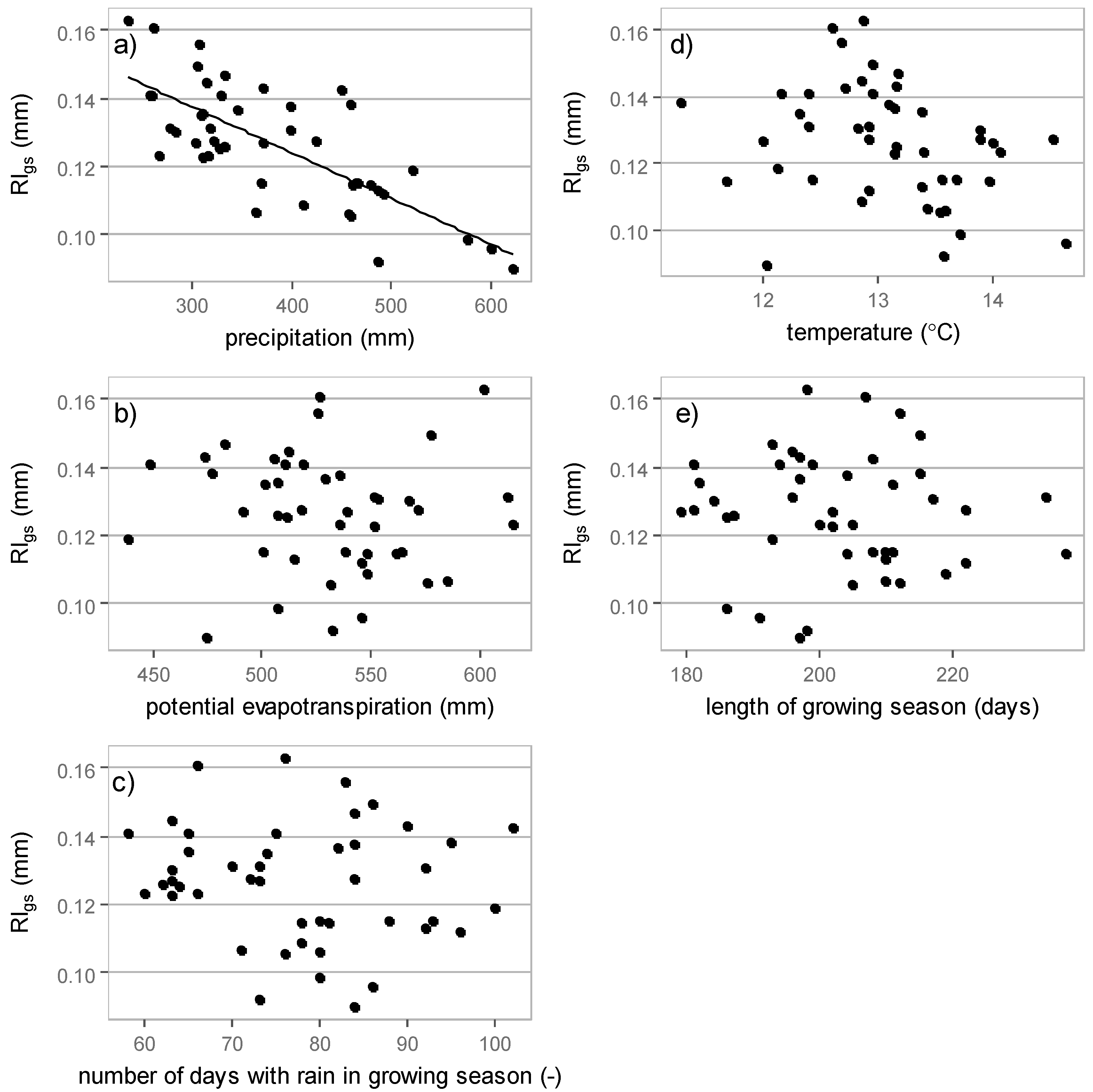
3.3.1. Growing Season Interception

Calculated absolute interception in the growing season ranged from 27.6 mm to 55.0 mm, with a mean of 39.3 mm. The part of the rain that was intercepted (relative interception) ranged from 9.0% to 16.3%, with a mean of 12.6%. Extreme values were observed in different months for both type of interception.
The relation between absolute interception in the growing season and hydrological and climatic variables is presented in Figure 6. The relation between the number of days with rain in the growing season and the length of the growing season is positive, while the relation between potential evapotranspiration and temperature is conversely negative. This relation is observed because, in years with high potential evapotranspiration, the sum of precipitation is low, and the total amount of water that can be intercepted by plants understandably drops. Correlation coefficients (R) are compared in Table 3. The highest correlation was obtained for number of days with rain in the growing season (R = 0.88), while a weak but significant correlation was also obtained for precipitation (R = 0.72). The quadratic relation with precipitation shows that in wet years (precipitation above 550 mm), intercepted water cannot evaporate between rain episodes (because of high humidity that leads to slow evaporation) and interception rates start to drop after the threshold precipitation value is exceeded. Other meteorological variables (potential evapotranspiration, temperature and the length of the growing season) were not significantly correlated with the absolute rainfall interception in the growing season.
The relationship of relative interception in the growing season to hydrological and climatic variables is showed in Figure 7. All relations are negative. Coefficients of correlation (R) are compared in Table 3. The highest correlation was obtained for precipitation (R = 0.75). Other meteorological variables (potential evapotranspiration, temperature, number of days with precipitation in the growing season, and length of growing season) were not significantly correlated with the relative interception in the growing season.

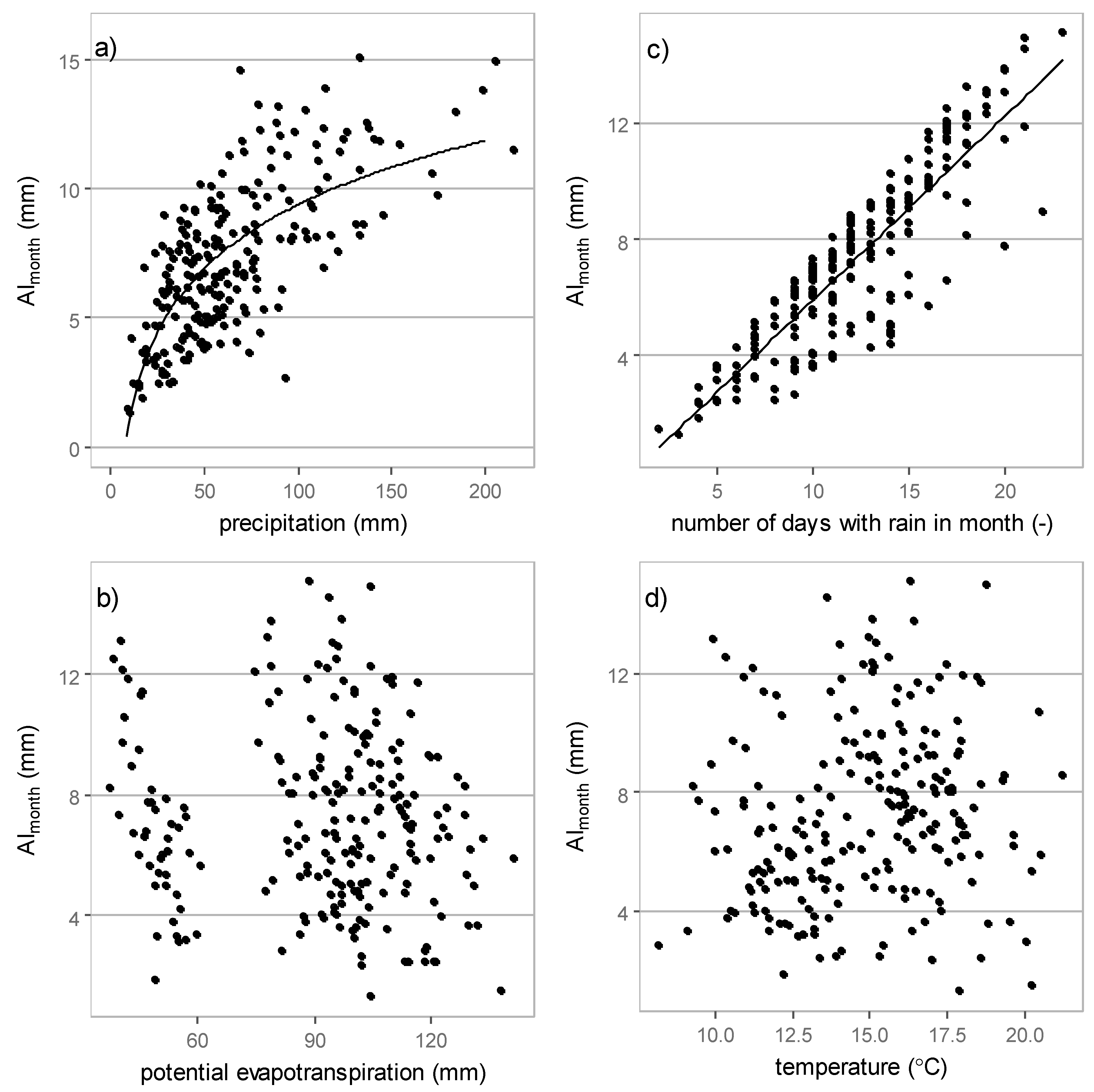
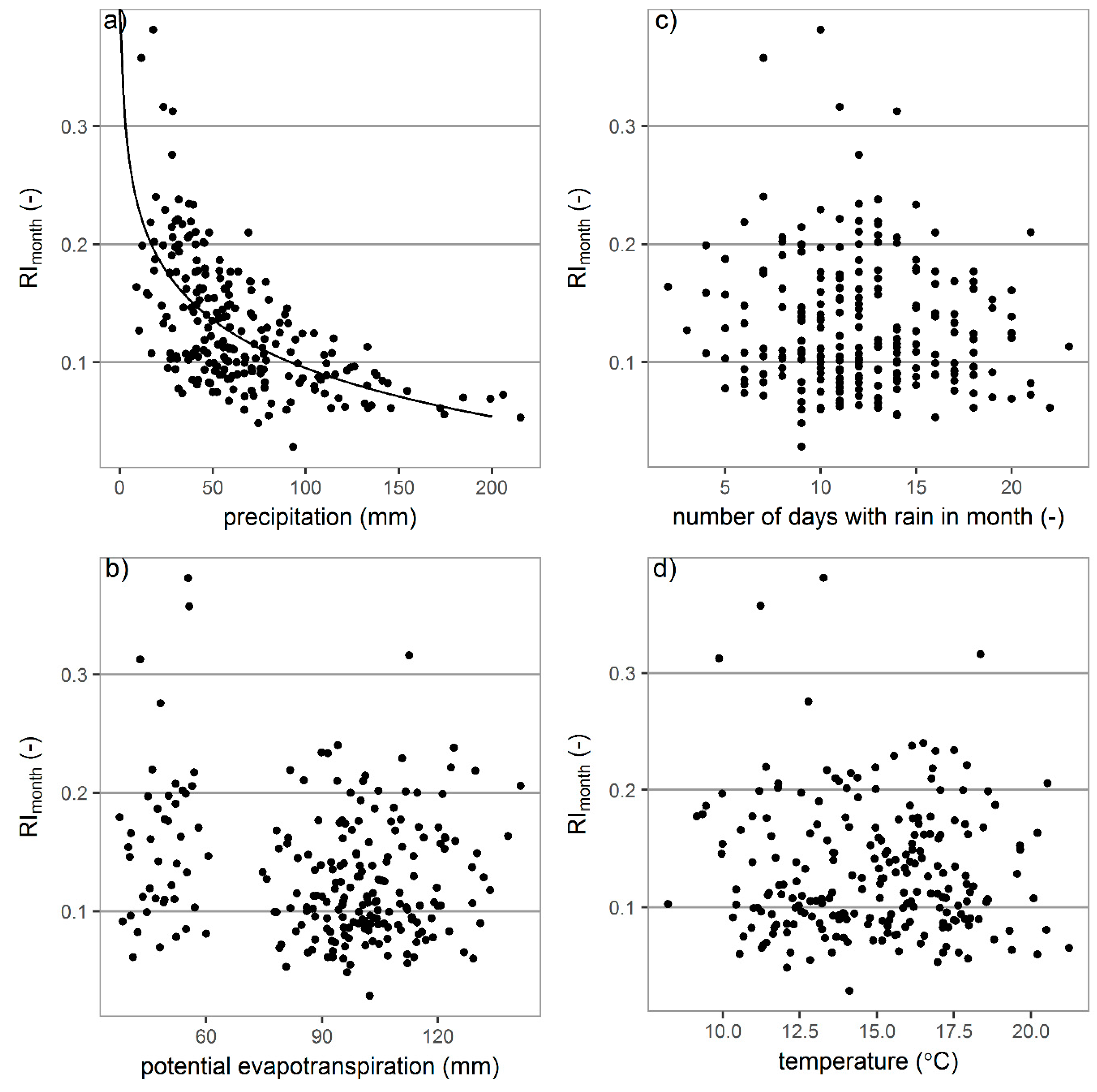
3.3.2. Monthly Interception

Calculated monthly absolute interception in the growing season ranged from 1.32 mm to 15.07 mm with a mean of 7.25 mm. The part of the rain that was intercepted (relative interception) ranged from 3.8% to 38.2% with a mean of 13.0%.
The relation between monthly absolute interception and observed meteorological elements is shown in Figure 8. Correlation coefficients (R) are compared in Table 4, separately for single months and overall for all months together. A high correlation was observed for the number of days with precipitation per month. Overall, R was 0.88, but, for single months, R is higher with figures ranging from 0.92 in May to 0.98 in August. Also significant, but much weaker, was the correlation of monthly AImonth with monthly sum of precipitation (R = 0.69). In September and July, R is 0.71 and 0.74, respectively, while for other months the R values are slightly lower. The overall correlation with potential evapotranspiration is irrelevant, but, for single months, the trend is significant and is up to 0.73 in July.
The relation between relative interception and observed meteorological elements is shown in Figure 9. Correlation coefficients (R) are compared in Table 4, separately for single months and overall for all available data. A significant correlation of relative interception was observed only for precipitation, but overall R is only 0.62, with a maximum of 0.77 in June.

4. Discussion

4.1. Maximum Canopy Storage

Investigation of maximum canopy storage on wetlands is not common. Based on what was observed in the literature, values between 0.2 mm and 1 mm are used, for example in the WetSpa model [17]. In this research, the smallest value of maximum canopy storage is 0.19 mm, but the upper limit of the result is higher than 1 mm, reaching 1.61 mm (Table 1). Another research conducted in the Lower Biebrza Valley (to the south of the study site) shows that, for selected species, maximum canopy storage can range from 0.87 mm to 7.37 mm [45]. When compared with our work, results presented in [42] seems to be overestimated. This large variability is caused by the high biodiversity in the natural wetland ecosystem. We also would like to note that the sampling sizes and submerging techniques for the other study are different. In this study, each plant sample of 25 cm × 25 cm grid has been split for individuals’ plants and measurement taken one by one, but, in [45], the whole plant sample in the 10 cm × 10 cm square has been submerged, which leads to a better generalisation of results in this study.
Most of the related works have been focused on grasslands and meadows, where plants are similar in morphology. For 27 alpine plant species found in the Glacier Lakes in Wyoming, the maximum canopy storage was maximally 0.05 mm [52]. On the other hand, for nine herbaceous species in the Alps, the observed values ranged from 0.13 mm to 3.14 mm [19]. In the Bodega Marine Reserve (California), for 18 clover species, the maximum canopy storage ranged from 0.13 mm to 0.36 mm [5]. In comparison, the results for wetland vegetation in this study fall in the middle.
Maximum canopy storage is in general lower for wetland plants than for the forest. For example, in [53], the maximum canopy storage for a Douglas-fir forest (>450 years old) located within the Gifford Pinchot National Forest (southern Washington) equals 3.32 mm, but, in the same study for a young Douglas-fir forest (20–25 years old), the value was much smaller at 1.4 mm, which is comparable to the extreme values shown in this study. In [54], a Douglas-fir forest in Speulderbos in the centre of the Netherlands has obtained higher values, such as 2.4 mm. However, some researchers have reported similar results of wetland vegetation for P. sitchensis in Great Britain (0.75 mm [55]) or even smaller for Pinus sp. in the Bray forest located 20 km southwest of Bordeaux, with a range of 0.50 to 0.55 mm [56]. Hence, this study shows that maximum canopy storage for wetland plants communities is smaller than for forests, but, for some specific wetland sites, it intercepts more water than forest.

4.2. Interception Losses

Maximum canopy storage provides information on the maximum amount of water that can be held by plants during a rainfall event. To investigate the influence of interception on water balance, we need the meteorological information about precipitation and evapotranspiration. With these values, it is possible to estimate interception losses in a given period of time.
Most research on interception losses is focused on forests [57]. Generally, interception losses in tree canopies represent 9% to 36% of the gross rainfall [58,59]. It has been estimated the rainfall interception losses is up to 48% of gross rainfall for the Corsican pine stands [34]. For upland forests in England, the interception losses amount to 35% in areas with an annual rainfall of more than 1000 mm, but it is reported that the loss is higher in areas with lower rainfall with 500–600 mm, amounting to about 40–50% [60]. For the mountainous areas in Poland, interception losses amount to 30% for both coniferous and deciduous forests where the annual rainfall ranged from 560 mm to 740 mm [61]. For wetland plants investigated in this study, the amount of interception losses is lower than values for forests (mean equal to 12.6% of rainfall), but, as with trees, higher gross rainfall was associated with lower interception losses. In the wettest growing season (sum of precipitation 621 mm), interception losses amount to only 9% of gross rainfall, while, in the driest growing season (sum of precipitation 235 mm), interception losses are almost twice as high and amount to 16.3% of the gross rainfall.
There are fewer studies conducted on interception losses for grass or other herbaceous plants, and with those few studies, their results show very high variability. In one study conducted in Texas, the interception losses for Curlymesquite grass were estimated as 10.8% of annual rainfall, while interception losses for Sideoats grama grass were estimated at 18.1% of annual rainfall [21]. In another study conducted in Australia, higher values were observed for Curly Mitchell grass at 32% of annual rainfall [31]. The study area in [21] has a mean annual precipitation of 609 mm, while, in [31], it is 255 mm. In our study for interception losses values of wetland plants, this area has a mean annual precipitation of 552 mm and lies between values of the two previously mentioned studies. These suggest that annual rainfall is an important factor and can lead to big variations in estimation of interception losses.
Our study confirmed that there are different driving factors of maximum canopy storage and interception losses. Maximum canopy storage depends on plant morphology and is highly varied across the same plant types, which can be seen by high standard deviation of field measurements and it is confirmed by different studies carried out in Biebrza Valley [36,45]. In addition, when maximum canopy storage was calculated for the entire plant communities (in the measuring squares) for the selected times of growing season, high variability is still observed where the mean values do not differ significantly. Meanwhile, interception losses are driven by hydrological and climatic variables, not just plant morphology and phenology (expressed by maximum canopy storage).
Interception losses were calculated with daily time step, based on precipitation, potential evapotranspiration and maximum canopy storage. Thus, the obtained values of interception losses must be affected by those processes. However, daily values were then used to calculate relationship of interception losses in growing season and month time scales. For these two time scales, more factors were taken into account and this factor: maximum storage capacity and precipitation distribution over time play an important role in values of monthly or growing season interception losses. Our results show that there is a high correlation between growing season and monthly interception losses and the number of days with precipitation in a given period. Furthermore, precipitation is highly correlated with interception losses.
Based on the data from 1971 to 2015, we observe a trend of increasing number of days with precipitation, at a rate of 0.4 days/year. The R of days of raining and absolute interception losses is very high at 0.88. Therefore, it is reasonable to expect the interception losses will be higher in the future. Our projection is it will be increased by 7.2 mm till 2050 and by 17.4 mm till 2100.
If the trends in our collected meteorological data remain the same in the future, a great impact on interception is anticipated. A potential huge increase in interception losses will in turn affect water balance. In our study area, there is no significant increase in precipitation over the years. However, for study areas where change in precipitation is significant, this change then needs to be considered in the projection/estimation of interception.

5. Conclusions

Based on one year’s measurements of maximum canopy storage for wetland plant communities, interception losses for the 1971–2015 period were estimated using meteorological elements. For both months and growing seasons, the mean value was around 13% gross precipitation, which shows that interception cannot be neglected in such areas and should be taken into account with more care in hydrological modelling.
One essential process in interception losses estimation is precipitation. The total sum of precipitation in the investigated period highly affected the estimation of interception. However, more important is the time distribution of precipitation, and the results show that the number of days with precipitation in the growing seasons is most strongly correlated with annual absolute rainfall interception. Even higher correlations are observed for monthly absolute interception. The fact that precipitation characteristics are driven by climate change makes rainfall interception an important parameter to consider in water balance studies.
Because interception losses are calculated based on daily values of climate and hydrological variables, its dependence on the latter is natural. However, the relation between interception losses with parameters is made in different time scales (in months and growing season) and we should look at all other processes such as distribution of rainfall over time and changes in maximum storage capacity. These observations enable us to project future trends of rainfall interception.
For annual and monthly relative interception, no strong correlations with meteorological elements were observed. Nonetheless, interception is a complex phenomenon that depends not only on meteorological conditions, but also on plant morphology. Hence, still more comprehensive research should be performed to fully understand the interception process itself and its influence on the whole ecosystem.

Acknowledgments

The research was conducted within the scope of research grant NCN2012/05/B/NZ9/03467 “INterception-TRanspiration-EVaporation; interdependencies of hydrological processes in WETland ECOsystems (INTREV-WetEco)”. The authors would like to thank Jonathan C.-W. Chan from Vrije Universiteit Brussel for his help in preparing the final version of this manuscript.

Author Contributions

Wojciech Ciężkowski conducted the field measurements, prepared the manuscript and analyzed the data; Tomasz Berezowski conducted the field measurement, supervised the first author, suggested the methodology, cooperated in data analysis and reviewed the manuscript; Małgorzata Kleniewska conducted the field measurements, processed the data, discussed methodology, and reviewed the manuscript; Sylwia Szporak-Wasilewska and Jarosław Chormański conducted the field measurements, discussed methodology and reviewed the manuscript.

Conflicts of Interest

The authors declare no conflict of interest.

References

  1. Wood, M.K.; Jones, T.L.; Vera-Cruz, M.T. Rainfall interception by selected plants in the Chihuahuan desert. J. Range Manag. 1998, 51, 91–96. [Google Scholar] [CrossRef]
  2. Van Dijk, A.; Bruijnzeel, L.A. Modelling rainfall interception by vegetation of variable density using an adapted analytical model. Part 1. Model description. J. Hydrol. 2001, 247, 230–238. [Google Scholar] [CrossRef]
  3. Muzylo, A.; Llorens, P.; Valente, F.; Keizer, J.J.; Domingo, F.; Gash, J.H.C. A review of rainfall interception modelling. J. Hydrol. 2009, 370, 191–206. [Google Scholar] [CrossRef]
  4. Campbell, C.L.; Madden, L.V. Introduction to Plant Disease Epidemiology; John Wiley & Sons: New York, NY, USA, 1990. [Google Scholar]
  5. Bradley, D.J.; Gilbert, G.S.; Parker, I.M. Susceptibility of clover species to fungal infection: The interaction of leaf surface traits and environment. Am. J. Bot. 2003, 90, 857–864. [Google Scholar] [CrossRef] [PubMed]
  6. Brueggemann, E.; Spindler, G. Wet and dry deposition of sulphur at the site melpitz in East Germany—In memorium dedicated to wolfgang rolle. Water Air Soil Pollut. 1999, 109, 81–99. [Google Scholar] [CrossRef]
  7. Wesely, M.L.; Sisterson, D.L.; Jastrow, J.D. Observations of the chemical-properties of dew on vegetation that affect the dry deposition of SO2. J. Geophys. Res. Atmos. 1990, 95, 7501–7514. [Google Scholar] [CrossRef]
  8. Brewer, C.A.; Smith, W.K. Patterns of leaf surface wetness for montane and subalpine plants. Plant Cell Environ. 1997, 20, 1–11. [Google Scholar] [CrossRef]
  9. Hanba, Y.T.; Moriya, A.; Kimura, K. Effect of leaf surface wetness and wettability on photosynthesis in bean and pea. Plant Cell Environ. 2004, 27, 413–421. [Google Scholar] [CrossRef]
  10. Savenije, H.H.G. The importance of interception and why we should delete the term evapotranspiration from our vocabulary. Hydrol. Process. 2004, 18, 1507–1511. [Google Scholar] [CrossRef]
  11. Grayson, R.B.; Moore, I.D.; McMahon, T.A. Physically based hydrologic modeling: 1. A terrain-based model for investigative purposes. Water Resour. Res. 1992, 28, 2639–2658. [Google Scholar] [CrossRef]
  12. Garrote, L.; Bras, R.L. A distributed model for real-time flood forecasting using digital elevation models. J. Hydrol. 1995, 167, 279–306. [Google Scholar] [CrossRef]
  13. Reggiani, P.; Rientjes, T.H.M. Flux parameterization in the representative elementary watershed approach: Application to a natural basin. Water Resour. Res. 2005, 41, 18. [Google Scholar] [CrossRef]
  14. Liu, Z.Y.; Todini, E. Towards a comprehensive physically-based rainfall-runoff model. Hydrol. Earth Syst. Sci. 2002, 6, 859–881. [Google Scholar] [CrossRef]
  15. Beven, K.; Kirkby, M.J. A physically based, variable contributing area model of basin hydrology/un modèle à base physique de zone d’appel variable de l’hydrologie du bassin versant. Hydrol. Sci. J. 1979, 24, 43–69. [Google Scholar] [CrossRef]
  16. Abbot, M.; Bathurst, J.; Cunge, J.; O’Connell, P.; Rasmussen, J. An introduction to the European hydrologic system-systeme hydologique Europeen, ”She”, 1: History and philosophy of a physically based, distributed modelling system. J. Hydrol. 1990, 87, 45–59. [Google Scholar] [CrossRef]
  17. Liu, Y.; De Smedt, F. Wetspa extension, a gis-based hydrologic model for flood prediction and watershed management. Vrije Universiteit Brussel Belgium 2004, 1, e108. [Google Scholar]
  18. Grah, R.F.; Wilson, C.C. Some components of rainfall interception. J. For. 1944, 42, 890–898. [Google Scholar]
  19. Wohlfahrt, G.; Bianchi, K.; Cernusca, A. Leaf and stem maximum water storage capacity of herbaceous plants in a mountain meadow. J. Hydrol. 2006, 319, 383–390. [Google Scholar] [CrossRef]
  20. Yu, K.L.; Pypker, T.G.; Keim, R.F.; Chen, N.; Yang, Y.B.; Guo, S.Q.; Li, W.J.; Wang, G. Canopy rainfall storage capacity as affected by sub-alpine grassland degradation in the Qinghai-Tibetan Plateau, China. Hydrol. Process. 2012, 26, 3114–3123. [Google Scholar] [CrossRef]
  21. Thurow, T.L.; Blackburn, W.H.; Warren, S.D.; Taylor, C.A. Rainfall interception by midgrass, shortgrass, and live oak mottes. J. Range Manag. 1987, 40, 455–460. [Google Scholar] [CrossRef]
  22. Jetten, V.G. Interception of tropical rain forest: Performance of a canopy water balance model. Hydrol. Process. 1996, 10, 671–685. [Google Scholar] [CrossRef]
  23. Germer, S.; Elsenbeer, H.; Moraes, J.M. Throughfall and temporal trends of rainfall redistribution in an open tropical rainforest, south-western Amazonia (Rondonia, Brazil). Hydrol. Earth Syst. Sci. 2006, 10, 383–393. [Google Scholar] [CrossRef]
  24. Czikowsky, M.J.; Fitzjarrald, D.R. Detecting rainfall interception in an Amazonian rain forest with eddy flux measurements. J. Hydrol. 2009, 377, 92–105. [Google Scholar] [CrossRef]
  25. Holder, C.D. Rainfall interception and fog precipitation in a tropical montane cloud forest of Guatemala. For. Ecol. Manag. 2004, 190, 373–384. [Google Scholar] [CrossRef]
  26. Aboal, J.R.; Jimenez, M.S.; Morales, D.; Hernandez, J.M. Rainfall interception in laurel forest in the Canary Islands. Agric. For. Meteorol. 1999, 97, 73–86. [Google Scholar] [CrossRef]
  27. Dykes, A.P. Rainfall interception from a lowland tropical rainforest in Brunei. J. Hydrol. 1997, 200, 260–279. [Google Scholar] [CrossRef]
  28. Grelle, A.; Lundberg, A.; Lindroth, A.; Moren, A.S.; Cienciala, E. Evaporation components of a boreal forest: Variations during the growing season. J. Hydrol. 1997, 197, 70–87. [Google Scholar] [CrossRef]
  29. Shachnovich, Y.; Berliner, P.R.; Bar, P. Rainfall interception and spatial distribution of throughfall in a pine forest planted in an arid zone. J. Hydrol. 2008, 349, 168–177. [Google Scholar] [CrossRef]
  30. Sraj, M.; Brilly, M.; Mikos, M. Rainfall interception by two deciduous mediterranean forests of contrasting stature in Slovenia. Agric. For. Meteorol. 2008, 148, 121–134. [Google Scholar] [CrossRef]
  31. Dunkerley, D.L.; Booth, T.L. Plant canopy interception of rainfall and its significance in a banded landscape, arid western New South Wales, Australia. Water Resour. Res. 1999, 35, 1581–1586. [Google Scholar] [CrossRef]
  32. Tromble, J.M. Interception of rainfall by tarbush. J. Range Manag. 1983, 36, 525–526. [Google Scholar] [CrossRef]
  33. Kołodziej, J.; Liniewicz, K.; Bednarek, H. Intercepcja opadów atmosferycznych w łanach zbóż. Acta Agrophys. 2005, 6, 381–391. (In Polish) [Google Scholar]
  34. Rutter, A.J.; Robins, P.C.; Morton, A.J.; Kershaw, K.A. Predictive model of rainfall interception in forests. 1. Derivation of model from observations in a plantation of corsican pine. Agric. Meteorol. 1972, 9, 367–384. [Google Scholar] [CrossRef]
  35. Berezowski, T.; Chormański, J.; Kleniewska, M.; Szporak-Wasilewska, S. Towards rainfall interception capacity estimation using ALS LiDAR data. In Proceedings of the 2015 IEEE International Geoscience and Remote Sensing Symposium (IGARSS), Milan, Italy, 26–31 July 2015; pp. 735–738. [Google Scholar]
  36. Suliga, J.; Chormanski, J.; Szporak-Wasilewska, S.; Kleniewska, M.; Berezowski, T.; van Griensven, A.; Verbeiren, B. Derivation from the Landsat 7 NDVI and ground truth validation of LAI and interception storage capacity for wetland ecosystems in Biebrza Valley, Poland. In Proceedings of the SPIE Remote Sensing for Agriculture, Ecosystems, and Hydrology XVII, Toulouse, France, 22–24 September 2015. [Google Scholar]
  37. De Jong, S.M.; Jetten, V.G. Estimating spatial patterns of rainfall interception from remotely sensed vegetation indices and spectral mixture analysis. Int. J. Geogr. Inf. Sci. 2007, 21, 529–545. [Google Scholar] [CrossRef]
  38. Gomez, J.A.; Giraldez, J.V.; Fereres, E. Rainfall interception by olive trees in relation to leaf area. Agric. Water Manag. 2001, 49, 65–76. [Google Scholar] [CrossRef]
  39. Hoyningen-Huene, J.V. Die Interzeption des Niederschlages in Landwirtschaftlichen Pflanzenbeständen; Arbeitsbericht Deutscher Verband für Wasserwirtschaft und Kulturbau, DVWK: Braunschweig, Germany, 1981. [Google Scholar]
  40. Verbeiren, B.; Khanh Nguyen, H.; Wirion, C.; Batelaan, O. An earth observation based method to assess the influence of seasonal dynamics of canopy interception storage on the urban water balance. Belgeo 2016, 2016. [Google Scholar] [CrossRef]
  41. Wirion, C.; Ho, K.N.; Bauwens, W.; Verbeiren, B. Using remote sensing to describe urban surface properties for improved hydrological modelling. In Proceedings of the 10th International Urban Drainage Modeling Conference, Quebec, QC, Canada, 20–23 September 2015. [Google Scholar]
  42. Górniak, A. Klimat i termika wód powierzchniowych kotliny biebrzańskiej. In Kotlina Biebrzańska i Biebrzański Park Narodowy: Aktualny Stan, Zagrożenia i Potrzeby Czynnej Ochrony Środowiska; Ekonomia i Środowisko: Białystok, Poland, 2004. (In Polish) [Google Scholar]
  43. Kossowska-Cezak, U.; Olszewski, K.; Przybylska, G. Climate of the Biebrza Valley. Zesz. Probl. Postepow Nauk Rolniczych 1991, 372, 119–158. (In Polish) [Google Scholar]
  44. West, N.E.; Gifford, G.F. Rainfall interception by cool-desert shrubs. J. Range Manag. 1976, 29, 171–172. [Google Scholar] [CrossRef]
  45. Ignar, S.; Węglewska, A.; Szporak-Wasilewska, S.; Chormański, J. Spatial and temporal variability of the interception in the natural wetland valley, the lower Biebrza basin case study. Ann. Warsaw Univ. Life Sci.-SGGW Land Reclam. 2013, 45, 111–119. [Google Scholar] [CrossRef]
  46. Calder, I.R.; Hall, R.L.; Rosier, P.T.W.; Bastable, H.G.; Prasanna, K.T. Dependence of rainfall interception on drop size: 2. Experimental determination of the wetting functions and two-layer stochastic model parameters for five tropical tree species. J. Hydrol. 1996, 185, 379–388. [Google Scholar] [CrossRef]
  47. Szporak-Wasilewska, S.; Szatyłowicz, J.; Okruszko, T.; Ignar, S. Application of the surface energy balance system model (SEBS) for mapping evapotranspiration of extensively used river valley with wetland vegetation. Towards Horiz. 2013, 2020, 929–942. [Google Scholar]
  48. Allen, R.G.; Pereira, L.S.; Raes, D.; Smith, M. Crop evapotranspiration—guidelines for computing crop water requirements—FAO irrigation and drainage paper 56. FAO Rome 1998, 300, D05109. [Google Scholar]
  49. Gash, J.H.C. Analytical model of rainfall interception by forests. Q. J. R. Meteorol. Soc. 1979, 105, 43–55. [Google Scholar] [CrossRef]
  50. Kępińska-Kasprzak, M.; Mager, P. Thermal growing season in Poland calculated by two different methods. Ann. Warsaw Univ. Life Sci. Land Reclam. 2015, 47, 261–273. [Google Scholar] [CrossRef]
  51. McLeod, A.I. Kendall Rank Correlation and Mann–Kendall Trend Test, Version 2.2; The R Foundation for Statistical Computing: Vienna, Austria, 2015. [Google Scholar]
  52. Monson, R.K.; Grant, M.C.; Jaeger, C.H.; Schoettle, A.W. Morphological causes for the retention of precipitation in the crowns of alpine plants. Environ. Exp. Bot. 1992, 32, 319–327. [Google Scholar] [CrossRef]
  53. Pypker, T.G.; Bond, B.J.; Link, T.E.; Marks, D.; Unsworth, M.H. The importance of canopy structure in controlling the interception loss of rainfall: Examples from a young and an old-growth douglas-fir forest. Agric. For. Meteorol. 2005, 130, 113–129. [Google Scholar] [CrossRef]
  54. Klaassen, W.; Bosveld, F.; de Water, E. Water storage and evaporation as constituents of rainfall interception. J. Hydrol. 1998, 212, 36–50. [Google Scholar] [CrossRef]
  55. Gash, J.; Wright, I.; Lloyd, C.R. Comparative estimates of interception loss from three coniferous forests in Great Britain. J. Hydrol. 1980, 48, 89–105. [Google Scholar] [CrossRef]
  56. Loustau, D.; Berbigier, P.; Granier, A. Interception loss, throughfall and stemflow in a maritime pine stand. II. An application of gash’s analytical model of interception. J. Hydrol. 1992, 138, 469–485. [Google Scholar] [CrossRef]
  57. Dunkerley, D. Measuring interception loss and canopy storage in dryland vegetation: A brief review and evaluation of available research strategies. Hydrol. Process. 2000, 14, 669–678. [Google Scholar] [CrossRef]
  58. Hormann, G.; Branding, A.; Clemen, T.; Herbst, M.; Hinrichs, A.; Thamm, F. Calculation and simulation of wind controlled canopy interception of a beech forest in northern Germany. Agric. For. Meteorol. 1996, 79, 131–148. [Google Scholar] [CrossRef]
  59. Levia, D.F.; Keim, R.F.; Carlyle-Moses, D.E.; Frost, E.E. Throughfall and stemflow in wooded ecosystems. In Forest Hydrology and Biogeochemistry: Synthesis of Past Research and Future Directions; Levia, D.F., CarlyleMoses, D., Tanaka, T., Eds.; Springer: Dordrecht, The Netherlands, 2011; Volume 216, pp. 425–443. [Google Scholar]
  60. Calder, I.R. Evaporation in the Uplands; John Wiley & Sons Ltd.: Chichester, UK, 1990. [Google Scholar]
  61. Kozłowski, R.; Jóźwiak, M. Transformacja opadów atmosferycznych w strefie drzew wybranych ekosystemów leśnych w górach świętokrzyskich = the transformation of precipitation in the tree canopy in selected forest ecosystems of poland’s świętokrzyskie mountains. Przegl. Geogr. 2017, 89, 133–153. (In Polish) [Google Scholar] [CrossRef]
Figure 1. Study site area (a) location of study sites in Upper Biebrza Basin; (b) location of Upper Biebrza Basin in Poland; (c) exact location of two measured meadows.
Water 10 00041 g001
Figure 2. Meadows under extensive agricultural use ((a) in Summer; (b) in Autumn).
Water 10 00041 g002
Figure 3. Measured (dashed line) and mean of generated (solid line) daily maximum canopy storage.
Water 10 00041 g003
Figure 4. Measured values of maximum canopy storage for the three field campaigns.
Water 10 00041 g004
Figure 5. Perennial trends of (a) precipitation; (b) potential evapotranspiration; (c) temperature; (d) number of days with precipitation; (e) length of growing season.
Water 10 00041 g005
Figure 6. Relationship between absolute growing season interception (AIgs) and: (a) sum of precipitation; (b) sum of potential evapotranspiration; (c) number of days with rain; (d) mean temperature; (e) length of the growing season.
Water 10 00041 g006
Figure 7. Relationship between relative growing season interception and: (a) sum of precipitation; (b) sum of potential evapotranspiration; (c) number of days with rain; (d) mean temperature; (e) length of the growing season.
Water 10 00041 g007
Figure 8. Relationship between absolute month interception (AImonth) and: (a) sum of precipitation; (b) sum of potential evapotranspiration; (c) number of days with rain; (d) mean temperature.
Water 10 00041 g008
Figure 9. Relationship between relative month interception (RImonth) and: (a) sum of precipitation; (b) sum of potential evapotranspiration; (c) number of days with rain; (d) mean temperature.
Water 10 00041 g009
Table 1. Maximum canopy storage in mm H2O per unit area and in g H2O per sampling area measured in 3 field campaigns.
DateNumber of SamplesMaximum Canopy Storage
mm H2O per Unit Areag H2O per Sampling Area
Mean ± SDminmaxMean ± SDminmax
26–29 June280.74 ± 0.350.291.5446.4 ± 21.917.996.2
28–30 July190.63 ± 0.270.201.4439.5 ± 16.912.289.7
4–5 September210.85 ± 0.390.191.6153.2 ± 24.412.1100.6
Table 2. Annual and growing season means of measured meteorological elements, and slope of their trends.
Meteorological ParameterAnnual MeanTrend SlopeGrowing Season MeanTrend SlopeAnnual M-K Tau
precipitation (mm)552 **+0.15 mm/year383 **−0.02 mm/year0.062 **
potential evapotranspiration (mm)600 *+1 mm/year530 *+1.76 mm/year0.259 *
temperature (°C)6.9 *+0.02 °C/year13.1 *+0.02 °C/year0.259 *
number of days with precipitation (-)143 *+0.4 day/year78 **+0.18 day/year0.274 *
growing season length (-)204 *+0.37 day/year 0.272 *
Notes: * p-value ≤ 0.05; ** p-value > 0.05.
Table 3. Correlation coefficients for relation between growing season interception (absolute and relative) and meteorological elements.
Meteorological ElementAbsolute Interception (mm)Relative Interception (-)
precipitation0.72 *0.75 *
potential evapotranspiration0.45 *0.05 **
numbers of days with rain0.88 *0.13 **
temperature0.36 *0.28 *
growing season length0.30 *0.08 **
Notes: * p-value ≤ 0.05; ** p-value > 0.05.
Table 4. Statistically significant (p-value < 0.05) correlation coefficients for relation between growing season absolute interception (AI), relative interception (RI) and meteorological elements.
Meteorological ElementMayJuneJulyAugustSeptemberAll Data
precipitationAI0.680.620.740.670.710.69
RI0.600.770.700.650.590.62
potential evapotranspirationAI0.400.590.730.640.69*
RI***0.37**
numbers of days with rainAI0.920.980.970.980.970.88
RI******
temperatureAI*0.350.500.380.31*
RI******
Note: * statistically insignificant relation (p-value > 0.5).

