Rheology of Un-Sieved Concentrated Domestic Slurry: A Wide Gap Approach


Abstract
:
1. Introduction
2. Rheometry
2.1. Couette Inverse Problem
2.2. Tikhonov Regularisation
2.2.1. Numerical Method
2.2.2. Recovering Yield Stress
3. Methods and Materials
3.1. Experimental Procedure
3.2. Materials
3.3. Sample Preparation
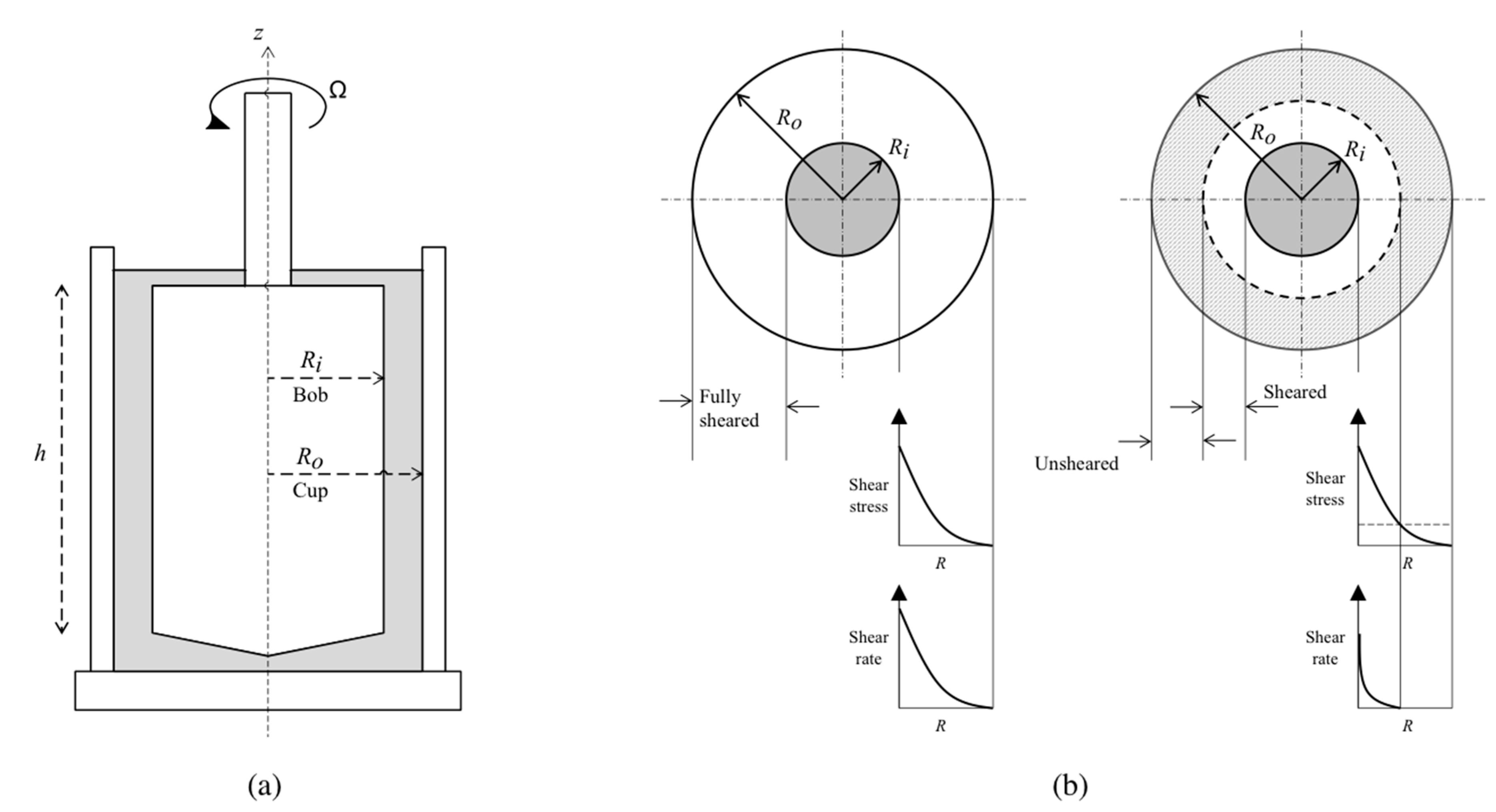
3.4. Wide Gap Rheometer
3.5. Model Parameter Estimation
4. Results and Discussion
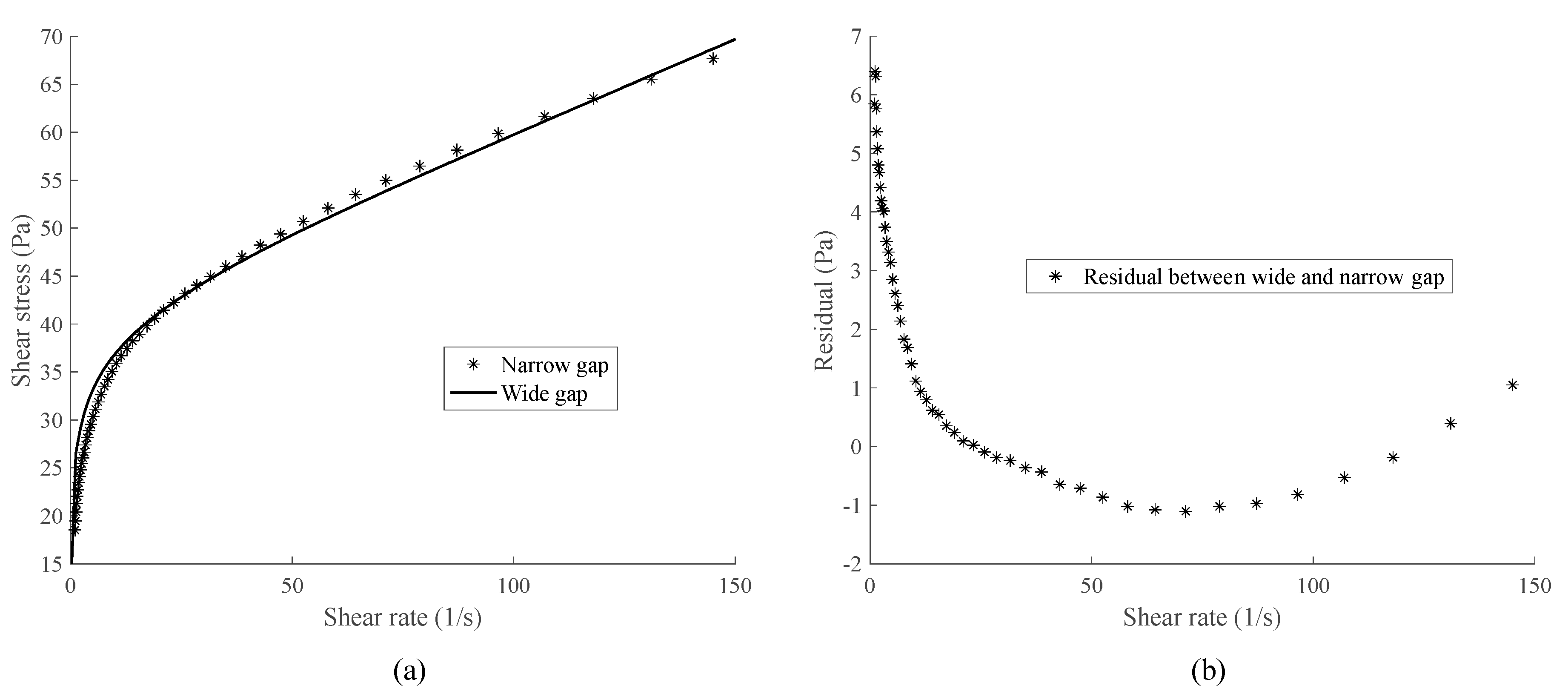
4.1. Choosing λ
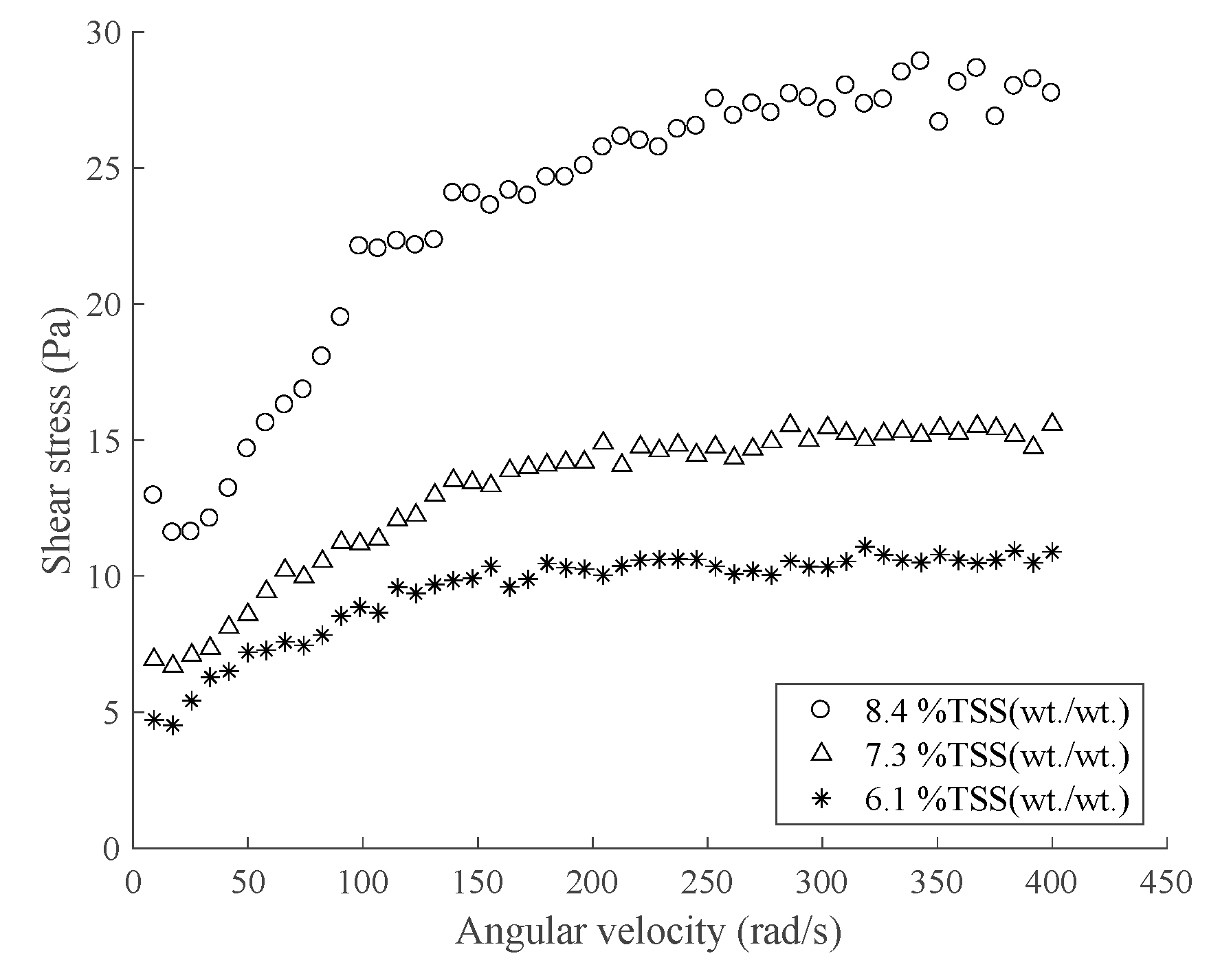
4.2. CDS Rheograms
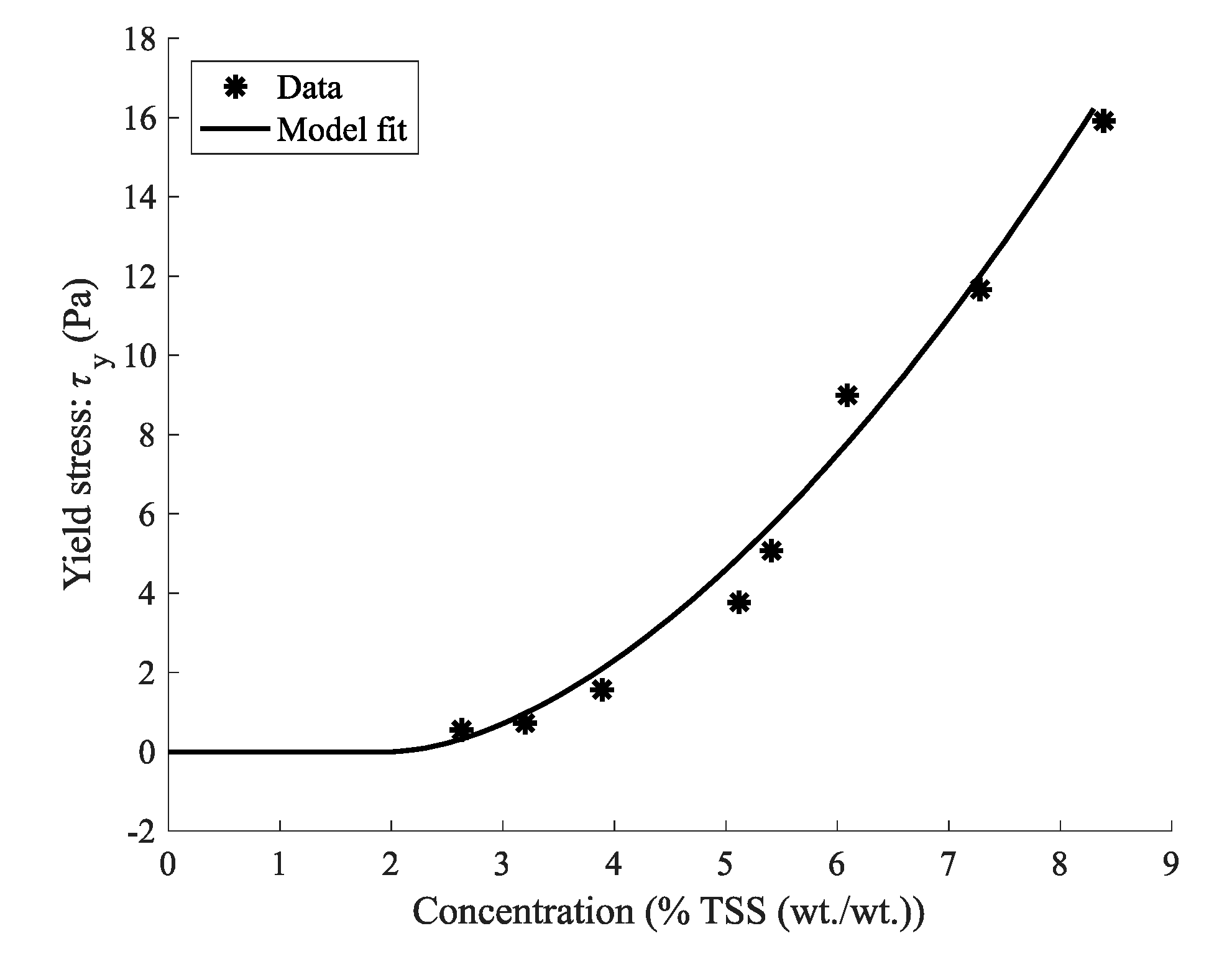
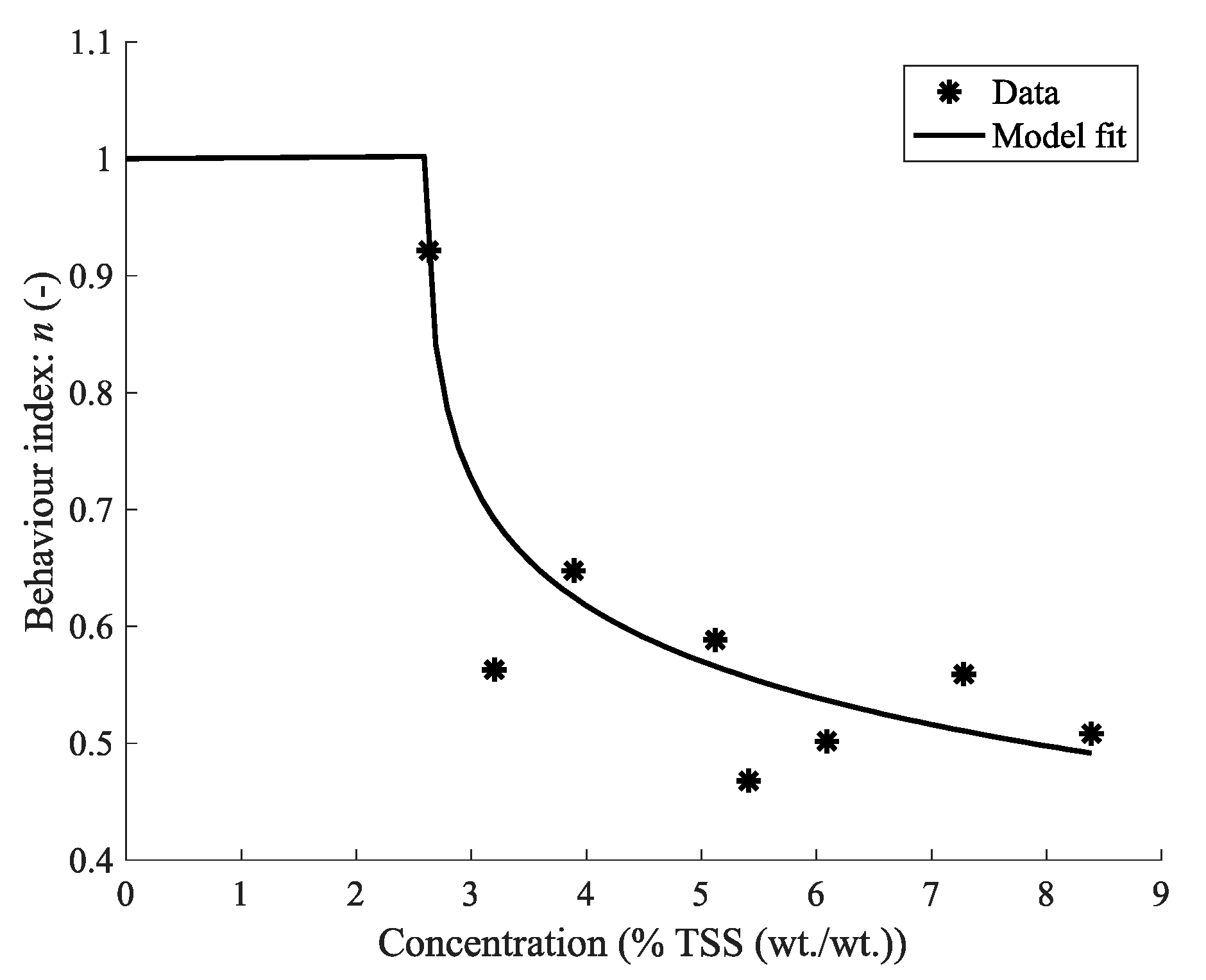
4.3. Effect of TSS Concentration: C
4.3.1. Yield Stress:
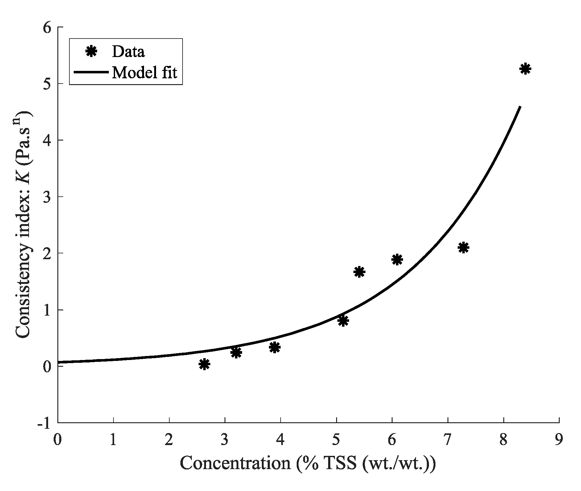
4.3.2. Consistency Index: K
4.3.3. Behaviour Index:
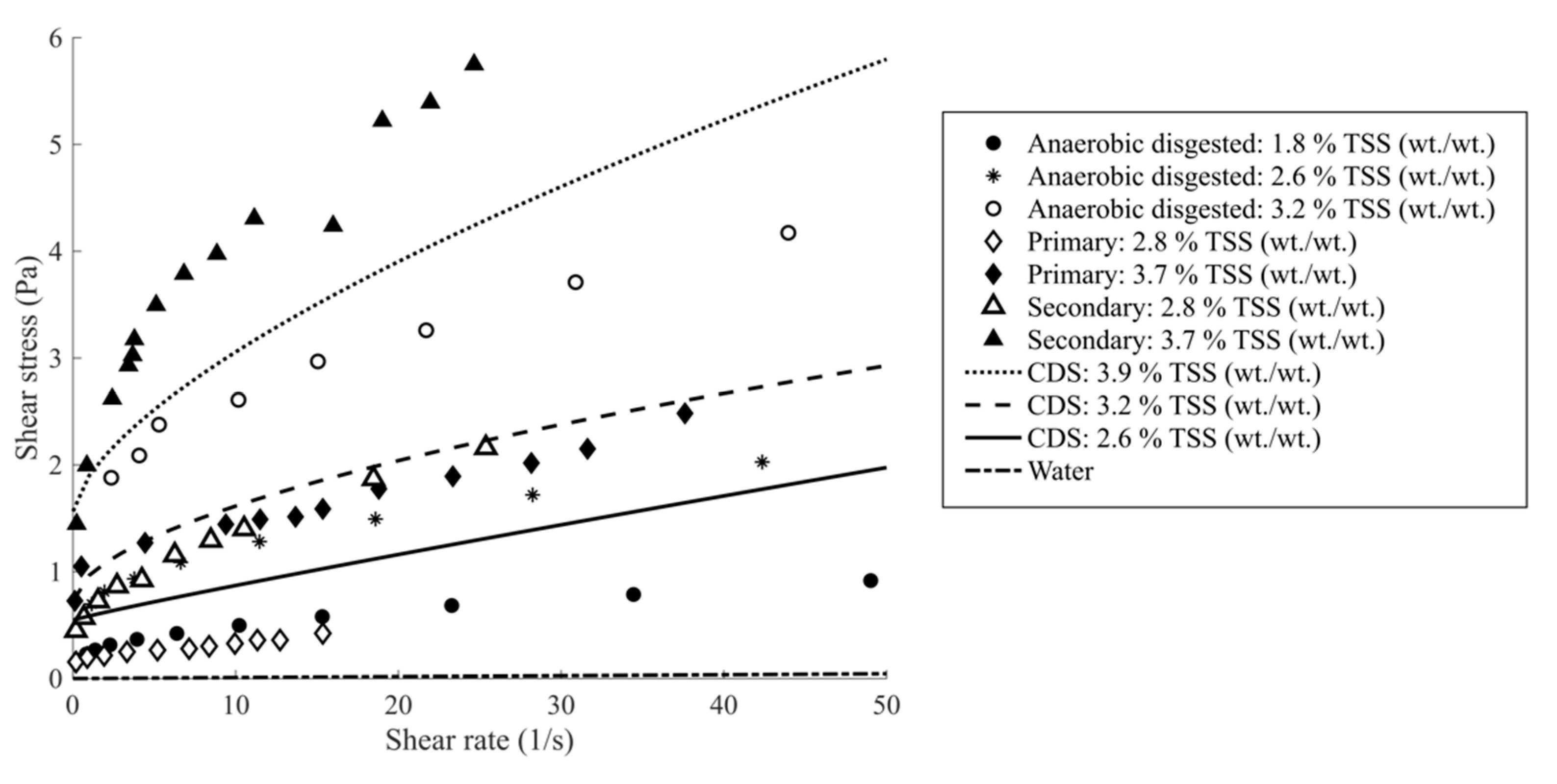
4.4. Comparison with Other Wastewater Slurries
5. Conclusions
Author Contributions
Funding
Acknowledgments
Conflicts of Interest
References
- Slatter, P.T. Transitional and Turbulent Flow of Non-Newtonian Slurries in Pipes. Ph.D. Thesis, University of Cape Town, Cape Town, South Africa, 1995. [Google Scholar]
- Thomas, A.D.; Wilson, K.C. New analysis of non-newtonian turbulent flowndashyield-power-law fluids. Can. J. Chem. Eng. 1987, 65, 335–338. [Google Scholar] [CrossRef]
- Chilton, R.; Stainsby, R.; Thompson, S. The design of sewage sludge pumping systems. J. Hydraul. Res. 1996, 34, 395–408. [Google Scholar] [CrossRef]
- Chhabra, R.P.; Richardson, J.F. Non-Newtonian Flow and Applied Rheology: Engineering Applications; Butterworth-Heinemann: Oxford, UK, 2011; ISBN 0080951600. [Google Scholar]
- AL-Behadili, A.J.M.; Sellier, M.; Nokes, R.; Moyers-Gonzalez, M.; Geoghegan, P.H. Rheometry based on free surface velocity. Inverse Probl. Sci. Eng. 2018, 1–21. [Google Scholar] [CrossRef]
- Longo, S.; Di Federico, V.; Archetti, R.; Chiapponi, L.; Ciriello, V.; Ungarish, M. On the axisymmetric spreading of non-Newtonian power-law gravity currents of time-dependent volume: An experimental and theoretical investigation focused on the inference of rheological parameters. J. Nonnewton. Fluid Mech. 2013, 201, 69–79. [Google Scholar] [CrossRef]
- Di Federico, V.; Longo, S.; King, S.E.; Chiapponi, L.; Petrolo, D.; Ciriello, V. Gravity-driven flow of Herschel–Bulkley fluid in a fracture and in a 2D porous medium. J. Fluid Mech. 2017, 821, 59–84. [Google Scholar] [CrossRef] [Green Version]
- Gurung, A.; Haverkort, J.W.; Drost, S.; Norder, B.; Westerweel, J.; Poelma, C. Ultrasound image velocimetry for rheological measurements. Meas. Sci. Technol. 2016, 27, 94008. [Google Scholar] [CrossRef]
- Eshtiaghi, N.; Markis, F.; Yap, S.D.; Baudez, J.-C.; Slatter, P. Rheological characterisation of municipal sludge: A review. Water Res. 2013, 47, 5493–5510. [Google Scholar] [CrossRef] [PubMed]
- Van Wazer, J.R. Viscosity and Flow Measurement: A Laboratory Handbook of Rheology; Interscience Publishers: Geneva, Switzerland, 1963. [Google Scholar]
- Slatter, P.T. The rheological characterisation of sludges. Water Sci. Technol. 1997, 36, 9–18. [Google Scholar] [CrossRef]
- Dick, R.I.; Ewing, B.B. The rheology of activated sludge. J. Water Pollut. Control Fed. 1967, 543–560. [Google Scholar]
- Koseoglu, H.; Yigit, N.O.; Civelekoglu, G.; Harman, B.I.; Kitis, M. Effects of chemical additives on filtration and rheological characteristics of MBR sludge. Bioresour. Technol. 2012, 117, 48–54. [Google Scholar] [CrossRef] [PubMed]
- Mori, M.; Seyssiecq, I.; Roche, N. Rheological measurements of sewage sludge for various solids concentrations and geometry. Process Biochem. 2006, 41, 1656–1662. [Google Scholar] [CrossRef]
- Ratkovich, N.; Horn, W.; Helmus, F.P.; Rosenberger, S.; Naessens, W.; Nopens, I.; Bentzen, T.R. Activated sludge rheology: A critical review on data collection and modelling. Water Res. 2013, 47, 463–482. [Google Scholar] [CrossRef] [PubMed]
- Battistoni, P. Pre-treatment, measurement execution procedure and waste characteristics in the rheology of sewage sludges and the digested organic fraction of municipal solid wastes. Water Sci. Technol. 1997, 36, 33–41. [Google Scholar] [CrossRef]
- Battistoni, P.; Pavan, P.; Mata-Alvarez, J.; Prisciandaro, M.; Cecchi, F. Rheology of sludge from double phase anaerobic digestion of organic fraction of municipal solid waste. Water Sci. Technol. 2000, 41, 51–59. [Google Scholar] [CrossRef] [PubMed]
- Woolley, S.M.; Cottingham, R.S.; Pocock, J.; Buckley, C.A. Shear rheological properties of fresh human faeces with different moisture content. Water SA 2014, 40, 273–276. [Google Scholar] [CrossRef]
- Ancey, C. Solving the Couette inverse problem using a wavelet-vaguelette decomposition. J. Rheol. (N. Y.) 2005, 49, 441–460. [Google Scholar] [CrossRef]
- Chatzimina, M.; Gerogiou, G.; Alexandrou, A. Wall Shear Rates in Circular Couette Flow of a Herschel-BulkleyFluid. Appl. Rheol. 2009, 19, 34288. [Google Scholar]
- Krieger, I.M.; Elrod, H. Direct Determination of the Flow Curves of Non-Newtonian Fluids. II. Shearing Rate in the Concentric Cylinder Viscometer. J. Appl. Phys. 1953, 24, 134–136. [Google Scholar] [CrossRef]
- Leong, Y.K.; Yeow, Y.L. Obtaining the shear stress shear rate relationship and yield stress of liquid foods from Couette viscometry data. Rheol. Acta 2003, 42, 365–371. [Google Scholar] [CrossRef]
- Estellé, P.; Lanos, C.; Perrot, A. Processing the Couette viscometry data using a Bingham approximation in shear rate calculation. J. Nonnewton. Fluid Mech. 2008, 154, 31–38. [Google Scholar] [CrossRef] [Green Version]
- Yeow, Y.L.; Ko, W.C.; Tang, P.P.P. Solving the inverse problem of Couette viscometry by Tikhonov regularization. J. Rheol. 2000, 44, 1335–1351. [Google Scholar] [CrossRef]
- Association, A.P.H. Standard Methods for the Examination of Water and Wastewater; American Public Health Association (APHA): Washington, DC, USA, 2005. [Google Scholar]
- Thota Radhakrishnan, A.; van Lier, J.; Clemens, F. Rheological characterisation of concentrated domestic slurry. Water Res. 2018, 141, 235–250. [Google Scholar] [CrossRef] [PubMed]
- Chaudhuri, A.; Wereley, N.M.; Radhakrishnan, R.; Choi, S.B. Rheological parameter estimation for a ferrous nanoparticle-based magnetorheological fluid using genetic algorithms. J. Intell. Mater. Syst. Struct. 2006, 17, 261–269. [Google Scholar] [CrossRef]
- Rooki, R.; Ardejani, F.D.; Moradzadeh, A.; Mirzaei, H.; Kelessidis, V.; Maglione, R.; Norouzi, M. Optimal determination of rheological parameters for herschel-bulkley drilling fluids using genetic algorithms (GAs). Korea-Aust. Rheol. J. 2012, 24, 163–170. [Google Scholar] [CrossRef]
- Seyssiecq, I.; Ferrasse, J.-H.; Roche, N. State-of-the-art: Rheological characterisation of wastewater treatment sludge. Biochem. Eng. J. 2003, 16, 41–56. [Google Scholar] [CrossRef]
- Quemada, D. Rheological modelling of complex fluids. I. The concept of effective volume fraction revisited. Eur. Phys. J. Appl. Phys. 1998, 1, 119–127. [Google Scholar] [CrossRef]
- Markis, F.; Baudez, J.-C.; Parthasarathy, R.; Slatter, P.; Eshtiaghi, N. Rheological characterisation of primary and secondary sludge: Impact of solids concentration. Chem. Eng. J. 2014, 253, 526–537. [Google Scholar] [CrossRef]
- Baudez, J.C.; Markis, F.; Eshtiaghi, N.; Slatter, P. The rheological behaviour of anaerobic digested sludge. Water Res. 2011, 45, 5675–5680. [Google Scholar] [CrossRef] [PubMed]


© 2018 by the authors. Licensee MDPI, Basel, Switzerland. This article is an open access article distributed under the terms and conditions of the Creative Commons Attribution (CC BY) license (http://creativecommons.org/licenses/by/4.0/).
Share and Cite
Thota Radhakrishnan, A.K.; Van Lier, J.; Clemens, F. Rheology of Un-Sieved Concentrated Domestic Slurry: A Wide Gap Approach. Water 2018, 10, 1287. https://doi.org/10.3390/w10101287
Thota Radhakrishnan AK, Van Lier J, Clemens F. Rheology of Un-Sieved Concentrated Domestic Slurry: A Wide Gap Approach. Water. 2018; 10(10):1287. https://doi.org/10.3390/w10101287
Chicago/Turabian StyleThota Radhakrishnan, Adithya Krishnan, Jules Van Lier, and Francois Clemens. 2018. "Rheology of Un-Sieved Concentrated Domestic Slurry: A Wide Gap Approach" Water 10, no. 10: 1287. https://doi.org/10.3390/w10101287
APA StyleThota Radhakrishnan, A. K., Van Lier, J., & Clemens, F. (2018). Rheology of Un-Sieved Concentrated Domestic Slurry: A Wide Gap Approach. Water, 10(10), 1287. https://doi.org/10.3390/w10101287