Modelling Groundwater Flow with MIKE SHE Using Conventional Climate Data and Satellite Data as Model Forcing in Haihe Plain, China

Key Laboratory of Agricultural Water Resources, Hebei Key Laboratory of Agricultural Water-Saving, Center for Agricultural Resources Research, Institute of Genetics and Developmental Biology, Chinese Academy of Sciences, Shijiazhuang 050021, China
*
Author to whom correspondence should be addressed.
Water 2018, 10(10), 1295; https://doi.org/10.3390/w10101295
Submission received: 3 July 2018
/
Revised: 28 August 2018
/
Accepted: 17 September 2018
/
Published: 20 September 2018
(This article belongs to the Special Issue Applications of Remote Sensing and GIS in Hydrology)
Abstract
:In North China Plain, accurate spatial and temporal ET and precipitation pattern is very important in the groundwater resource assessment. This study demonstrated the potential for modelling ET and groundwater processes using remote sensing data for distributed hydrological modelling with MIKE SHE codes in the Haihe Plain, China. The model was successfully validated against independent groundwater level measurements following the calibration period and the model also provided a reasonable match of the lysimeter measurements of ET. The remote sensing data included ET derived from global radiation products of Fengyun-2C geostationary meteorological satellite (FY-2C) and FY-2C precipitation products. The comparisons show that precipitation is a critical factor for the hydrological response and for the spatial distribution of ET and groundwater flow. FY-2C precipitation products has a spatial resolution of about 11 km, which thus adds more spatial variability to the most important driving variable. The ET map based on FY-2C data has a higher spatial variability than that map based on conventional data, which are caused by higher resolution of ground information. The groundwater level changes in the aquifer system are shown in the quite different spatial patterns under two models, which is affected by the significant difference between two types of precipitation. In the Haihe Plain, accurate spatial and temporal ET pattern is very important in the groundwater resource assessment that determines the recharge to the saturated zone.
1. Introduction
In general, the surface and groundwater resources and their spatio-temporal variation and use are vaguely known which hinders proper water resources managements. These applications require an accurate prediction of hydrological variables spatially and temporally. Distributed hydrological models can provide the desired variables at required resolution [1,2]. MIKE SHE is a distributed and physically-based hydrological model developed by DHI Group, Inc., which delivers integrated modelling of groundwater, surface water, recharge [3] and evapotranspiration and has been widely used to study various water resource management problem [4,5,6,7]. We applied MIKE SHE to the part area of the alluvial plain of Mt. Taihang with an intensive crop growing, China to examine the components of the groundwater balance and to assess the impacts of crop water use and crop rotations on groundwater regime. However, the distributed nature of these models not only requires extensive data amounts for driving the models and for the parameterization of the land surface and subsurface but also requires that they should be calibrated and validated on a distributed basis [5,8,9]. Apart from land surface data (such as topographic, soil, land use and vegetation data, etc.), a hydrological model need the input of meteorological data including precipitation and reference evapotranspiration (ET). An accurate representation of meteorological data in space and time is critical for reliable predictions of the hydrological responses [10].
In order to obtain these kinds of meteorological data, people are struggling to set up global coverage of observing stations making surface measurements. However, there is a general lack of meteorological data in arid and semiarid regions. Generally, a county (or a city) has a public meteorological station in China and the area of a county or city ranges approximately 400 km2 to 1000 km2 in Haihe Plain, China. Figure 1 shows the meteorological stations that we received daily data from the China Meteorological Data Service Center. Compared to this, remote sensing (RS) has attractive advantage of an unprecedented spatial and temporal coverage of critical land surface and atmospheric data. Therefore RS data have been extensively used in groundwater modelling, especially in the region with a weak observation infrastructure [11,12,13,14]. RS has often been used in hydrological modelling as driving data or for parameterization [5,15,16,17,18,19]. Furthermore, actual ET or soil moisture estimated from remote-sensing data provide opportunities for assimilation in hydrological models and for filling spatio-temporal gaps for model calibration and validation [13,20,21,22].
In current study, the objective is to examine if remote-sensing data from the Fengyun-2C (FY-2C), a Chinese operational geostationary satellite, can improve the estimation of actual ET and groundwater level. We compared two distributed models based on RS inputs and conventional data for the Haihe Plain, China, where there is one of the most depleted aquifers in the world for crop growing depends on intensive irrigation [23,24]. FY-2C products including the daily precipitation and global radiation for potential evapotranspiration estimation applied in the distributed hydrological model. Meanwhile, the conventional distributed hydrological model also built up. It is expected that model results different both from distributed conventional hydrological model and RS hydrological model since there are important difference in deriving variables. In addition, the triangle method that is widely used to estimate the daily ET is introduce.
In this study, we developed, calibrated and validated an integrated and distributed hydrological model for the Haihe Plain based on available conventional data and information. Based on this calibrated hydrological model, the geostationary satellite FY-2C products were used as driving force for the second step. We compared the simulations results of the two models spatially and temporally. Further, the simulation results were compared to estimates of daily actual ET under an improved triangle method that is widely used based on MODIS and FY-2C data [25,26,27].
2. Materials and Methods
The MIKE SHE code was used to simulate the hydrological behaviour in the region. The spatial data available are shown in Figure 1. Due to the overlap of limited data, this study was carried out for three steps to achieve the comparison of conventional climate data and satellite data for hydrological forcing. First, the hydrological model was applied based on conventional climate data from 1 January 1996 to 9 June 2005. The model was calibrated from 1996 to 2002 and validated from 1996–2004. Then the simulation results from the 1st hydrological model were used as the hot start. FY-2C satellite products were used as input data for precipitation and potential ET for the hydrological model from 9 June 2005 to 30 August 2008. Meanwhile, the hydrological model based on conventional meteorological data was also simulated for the same period.
Total water balance, actual ET and groundwater level difference were used for model comparisons. The daily actual ET directly estimated from using the improved triangle method based on FY-2C and MODIS products were used to compare the actual ET from the two models.
2.1. Study Area
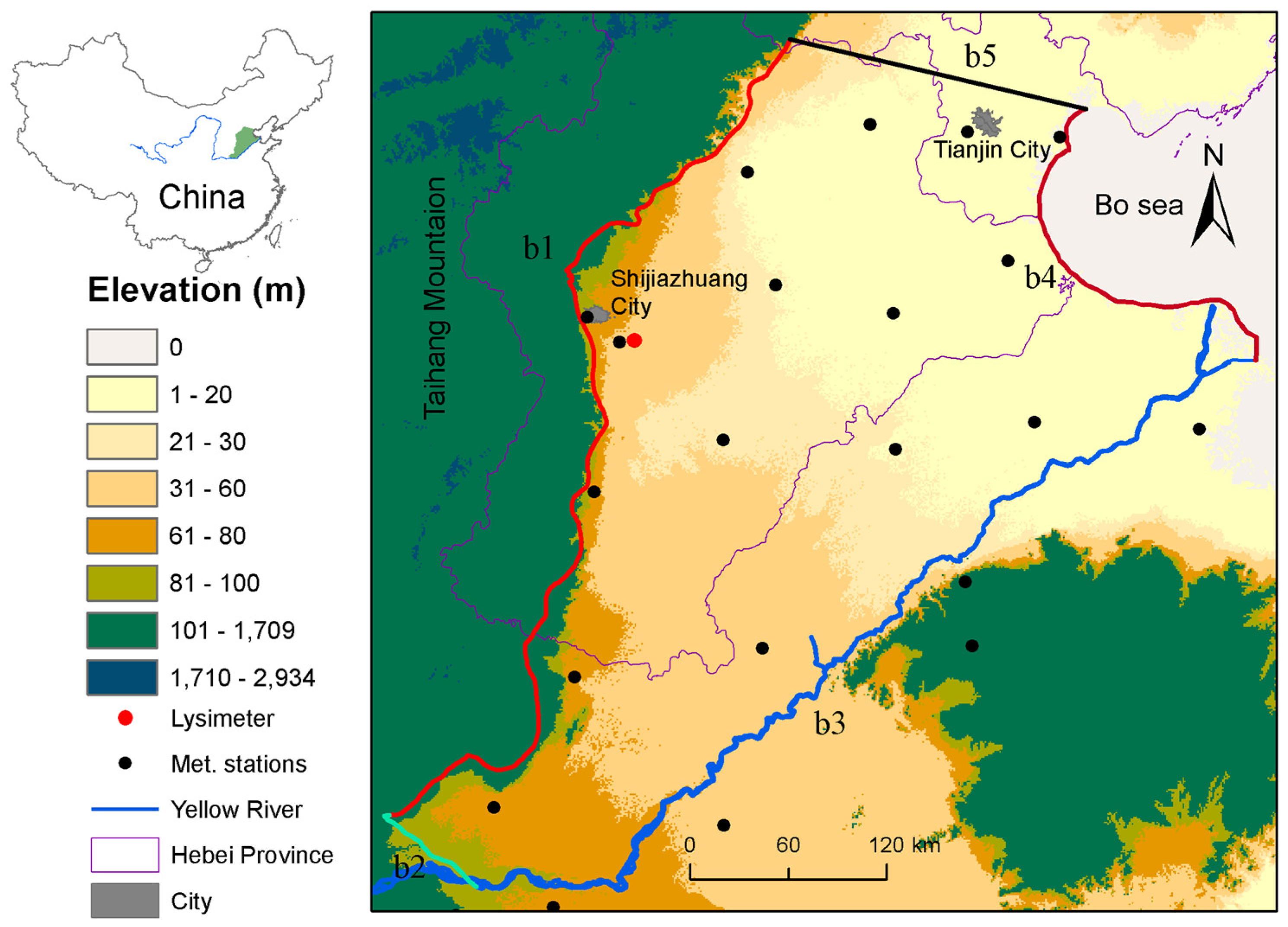
Haihe Plain is located in the north of the North China Plain (NCP), which is developed on alluvial deposits of Hai River. The plain is bordered on the north by the Yanshan Mountains, on the west by the Taihang Mountains, to the south flows the Yellow River and to the east fronts the Bohai Sea. The study area is located between 34.7°–39.6° N, 113.1°–119.1° E and covers most of the Haihe Plain (Figure 1). It covers an area of about 120,000 km2, most of which is less than 50 m above sea level. Winter wheat and summer corn are the main crops of grain produced and the yields of winter wheat and summer corn in more than half the counties in the Plain reached 6–7 ton/ha and 7–8 ton/ha respectively since the 1980s, which are the highest in the world. The normal annual precipitation generally ranges from 300 to 800 mm, with moderate rainfall of 400–600 mm. The monthly distribution of annual precipitation is uneven, with about 70 percent occurring within 3 months—from June to August. The yearly changes in annual precipitation are significant with the difference of precipitation during dry and wet years being as much as three to four times the amount. As runoff generated from upland areas has decreased significantly over the past decades, resulting in overexploitation of the regional water resources, serious water and eco-environmental problems have arisen. Haihe plain is one of regions that has suffered the highest exploitation and a serious shortage of water resources in NCP [24,28]. Since the 1970s, groundwater levels have declined significantly due to over-exploitation of groundwater, for example, average burial depth of ground water at Luancheng county, Shijiazhuang city, Hebei province, declined to 39.1 m from 8.5 m from 1975 to 2016.
Groundwater resources in the region mainly exist in Quaternary aquifers of depths up to 400 m. The aquifers are composed of unconsolidated pebble, gravel and sand. From west to east, the particles of the aquifers become finer, and the thickness of individual aquifers decreases. In the piedmont area to the west and the north of the plain, the aquifers are better recharged, more permeable, have good water quality and the water table is deep. In the middle part of the plain, the shallow freshwater aquifers are primarily fine sand. In the river mouth area of the Yellow River, both shallow and deep aquifers contain saltwater to various extents. The deep confined aquifers typically supply the major cities and industries while smaller cities and agriculture traditionally are supplied with water from shallow, unconfined aquifers. However, this is changing with agricultural wells now being deepened to maintain supplies [29].
2.2. Model Based on Conventional Data
2.2.1. MIKE SHE Model Code
This model coupled the unsaturated zone (UZ) and saturated zone flow together. MIKE SHE has three options for the evapotranspiration simulation, including Richards equation, Gravity flow and two-layer UZ. Due to the reasonable computing time, a rather simple evapotranspiration scheme: the two-layer water balance method [30] that predicts actual ET based on tim × 10-series of potential evapotranspiration computed from standard meteorological data was used. ET calculation is carried out in two steps: (1) calculate the potential evapotranspiration (ETp) and (2) calculate actual evapotranspiration (ETa). The potential evapotranspiration can be computed by reference evapotranspiration multiplying with the crop coefficient (Kc). Based on the FAO guidelines [31], Kc is the coefficient for crops growing under conditions of optimum fertility and soil moisture and achieving full production potential.
Actual ET depends on both the potential ET and the amount of water available to meet the potential ET. In the integrated model, water to meet ETp is supplied first from interception storage. If ETp exceeds interception storage, available ponded water will be supplied. If the ETp has not yet been satisfied, water is removed from the unsaturated zone. Finally, if ETp exceeds the water available from interception storage, ponded and water in the unsaturated zone, water will be supplied from the saturated zone. Water available in the saturated zone for the rest of ETp depends on the depth of water table. ETa is the sum of water available to ET from the above four processes.
The unsaturated zone is defined as the zone above the water table and below land surface. The thickness of the unsaturated zone varies as the water table fluctuates.
The main purpose of this simplified ET method is to calculate actual evapotranspiration and the amount of water that recharges the saturated zone. Saturated water flow (i.e., groundwater flow) is simulated by the two-dimensional equation using the finite difference method.
where Kxx, Kyy are hydraulic conductivity in x and y directions respectively; h is hydraulic head; Ss is specific storage coefficient; and Q represents the source/sink term (i.e., recharge, pumping, etc.).
2.2.2. Model Setup
The model setup is based on the model proposed for the partial area of the alluvial plain of Mt. Taihang [4],. Then we extended the model area to the total area of 120,000 km2 (Figure 1). The model is simulated on a 1 km by 1 km computational grid. The temporal resolution of the driving variables is 1 day.
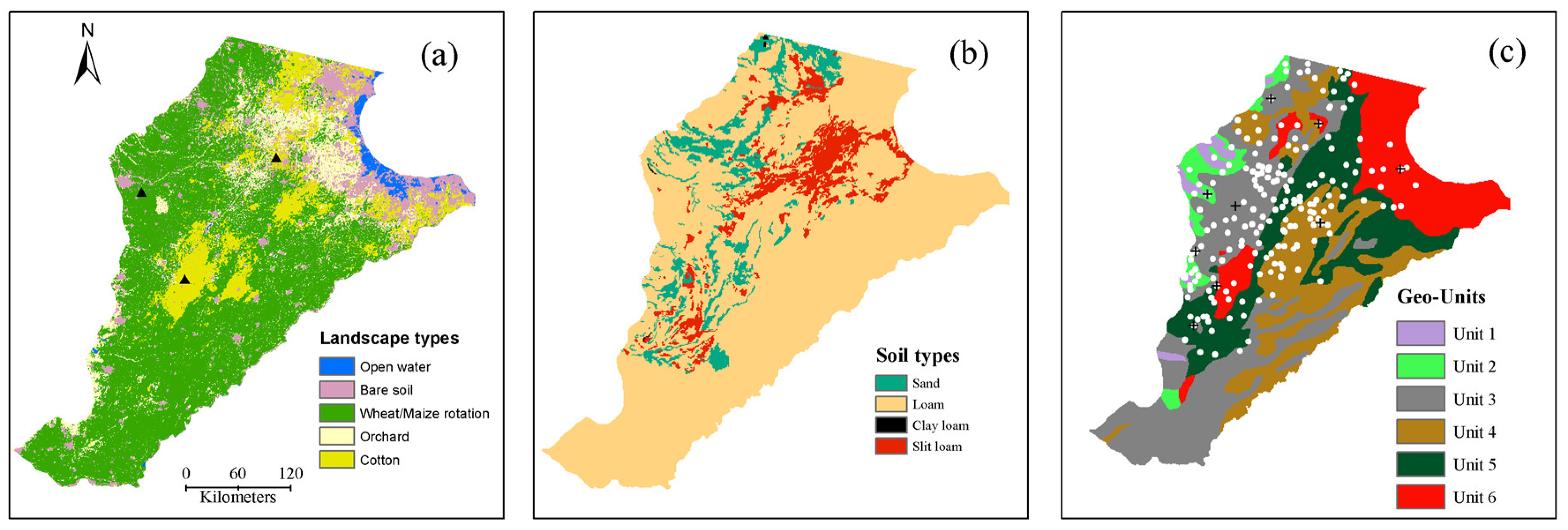
Table 1 lists the sources of the different data used in the study. Topography was generated from a Shuttle Radar Topography Mission (SRTM) topographical map with a resolution of 90 m and subsequently aggregated to 1 km. Remote-sensing precipitation products of FY-2C were provided by National Satellite Meteorological Center. FY-2C, has a Visible Infrared Spin Scan Radiometer with five spectral bands. And the acquisition time is one hour outside the rainy season and 30 min during the rainy season. The precipitation is estimated using the VIS-IR channels in combination with the rain gauge data [32]. The FY-2 VIS-IR channels observe cloud tops which give an indirect signal of rainfall underneath. The rainfall screening threshold and rainfall-estimation coefficients were geologically scattered depending on the distribution of the gauges by which they were calculated [33]. FY2 rainfall products in northern China were relatively reliable in performing the spatiotemporal distribution and diurnal variation of precipitation and the accuracy of FY2 RS precipitation product that was calibrated using ground observation data was higher than CMORPH products [34]. Conventional data from meteorological stations shown in Figure 1 were provided by the Chinese Meteorological Data Service in the form of daily values for precipitation, air temperature, vapour pressure, sunshine hours, relative humidity, and wind speed for the period 1996–2008. Reference ET was estimated using a version of the Penman-Monteith equation used in FAO irrigation and drainage paper [31], which has been recommended by FAO to represent potential evapotranspiration from a grass cover. The spatial area that each meteorological station represents in the model was computed from the Thiessen polygon method using ArcGIS, resulting in 22 areas of various sizes within which precipitation and reference ET is assumed uniform. In the model, we assume that all irrigation water is abstracted from groundwater. The land cover classification was divided into five classes: open water, farmland of winter wheat/summer maize, farmland of cotton, orchard, and bare soil (Figure 2a). It is assumed that the generated land cover classification is representative for the conditions throughout the simulation period. Irrigation is applied to areas with winter wheat/summer maize, cotton and fruit tree (orchard). The detailed description of the irrigation application and crop vegetation parameters were can be found in our previous study [4]. A soil map of the study area is shown in Figure 2b. The overall dominating soil type is loam and due to lack of data outside Hebei province we have assumed that this soil type is valid here. The hydraulic properties for the individual soil types were adopted from our previous study [4] and are given in Table 2.
θsat is the water content at saturation, θfc is the water content at field capacity, θwp is the water content at wilting point and Ks is the saturated hydraulic conductivity.
The boundary conditions for the groundwater system are defined as follows: The west and southwest boundaries along the Taihang Mountain range (b1 and b2 in Figure 1), which are considered as the main lateral inflow boundaries are defined with a specified constant and uniform gradient, which was estimated on the basis of previous studies [23,35,36]. The north-east boundary (b4 in Figure 1) is placed along the coastline and is specified as a fixed hydraulic head, corresponding to sea level (0 m). The north boundary (b5 in Figure 1) is placed such that it is parallel to the predominant flow direction and as such is specified as a no-flow boundary. The boundary along the Yellow River (b3 in Figure 1) is specified as a constant hydraulic head condition. The specified head varies along the river reach according to available topographical information.
In the model, we only simulate the groundwater dynamics of the shallow groundwater system, extending to a maximum depth of 150 m. The shallow groundwater system is here defined as the upper two layers of the aquifer system which is the primary source of water for irrigation. These two layers are hydraulically interconnected and due to limited information of the detailed geological settings, the layers in the model are considered as a single computational layer. The lower confinement of the upper aquifer system was determined from a geological map (scale: 1:500,000) of the Haihe Plain (Table 1). The aquifer was divided into six hydrogeological units (Figure 2c), based on a geological map of Haihe Plain (Table 1). From the geological characterization, all hydrogeological units are expected to have relatively high hydraulic conductivities and to be quite water-productive. Estimated values for horizontal hydraulic conductivity for the different units are listed in Table 3.
The initial groundwater levels for the simulation period (1 January 1996 to 31 December 2004) were established by interpolation of data from the 199 observation wells (Figure 2c). To ensure internal consistency, the initial water table configuration was subsequently modified manually by removing unrealistic observations and, furthermore, adjustments were made near the model boundaries such that the initial head configuration was consistent with the imposed boundary conditions. As the system is in a long-term transient state due to the long-term intensive groundwater pumping it was not possible to stabilize the model based on a warm-up period. However, the internal consistency of the initial conditions is a crucial factor for the accuracy of the simulation results.
2.2.3. Model Calibration and Validation
The model based on conventional meteorological data was calibrated and validated using measurements of groundwater heads in selected observation wells for the period 1996–2002 (see below for details). The parameter estimation/model calibration software PEST [37] was used for this purpose after an initial manual trial-and-error calibration. Subsequently, the model was validated against hydraulic heads measurements for the years 2003 and 2004. Hydraulic head measurements from 199 observation wells were used as calibration targets in the auto-calibration process. The observation wells were selected such that a uniform coverage was obtained within the Hebei province (Figure 1). The model cannot be constrained outside the province as no data were available here. Of the selected wells, 42 were measured daily while 157 were measured every 5th day. Prior to the auto-calibration, a sensitivity analysis was carried out to identify the most sensitive groundwater parameters. The calibration procedure did not include input parameters related to evapotranspiration and soil water flow, which were adopted from our precious study [4]. The parameters chosen for calibration are listed in Table 4. The hydraulic conductivities and specific yields for all hydrogeological units were included as well as the two imposed gradients in hydraulic heads at the upstream boundaries (b1 and b2). The hydraulic conductivities were log-transformed in the optimization process. Two measures were included in the objective function to be minimized during calibration: the root mean square error (RMSE) of hydraulic head h and the RMSE of the error of change in hydraulic head (dherror). RMSE of h is an aggregated measure that includes both the bias and the dynamic correspondence of the groundwater heads. RMSE of dh-error was introduced to represent situations where observed and simulated hydraulic heads are offset but the rates of change are similar. As long as the rate of change of observations and simulations are alike, the model response will be considered acceptable. dherror is defined as:
where Odif is the difference in observed hydraulic head from one year to the next, and Sdif is the difference in simulated head over the same period. We assigned a weight of 1/3 to the RMSE of heads and 2/3 to the RMSE of dherror in the composite objective function, taking into consideration the differences in absolute values of the two components.
The calibration was carried out for a 7-year period (1996–2002). This period includes both wet and dry years. Year 1996 was an exceptionally wet year with an annual precipitation at the Luancheng station of 774 mm; while year 1997 and 2001 were both dry with annual precipitations of 273 mm and 290 mm, respectively. Thus, the calibration period included seasons with different groundwater dynamics due to variations in recharge. The optimization results from the auto-calibration are listed in Table 4.
Since most parameters of the auto-calibration resulted in little changes from the initial values, the parameters with initial trial-and-error calibration are optimal for the current model setup. The parameters that were subject to most adjustments were specific yields that determine the dynamic response of the groundwater system and boundary gradients that determine the influx of groundwater and thus the water balance.
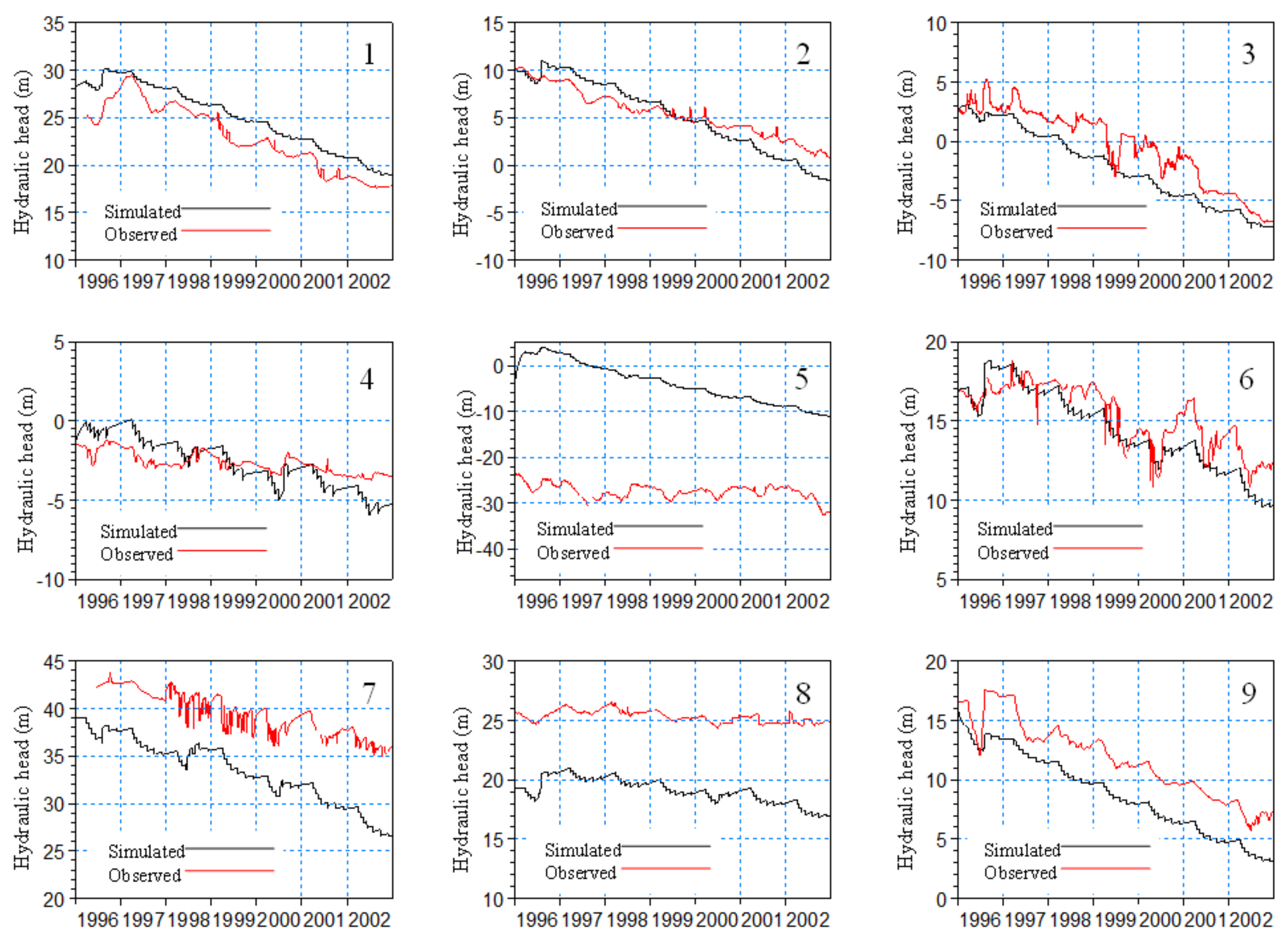
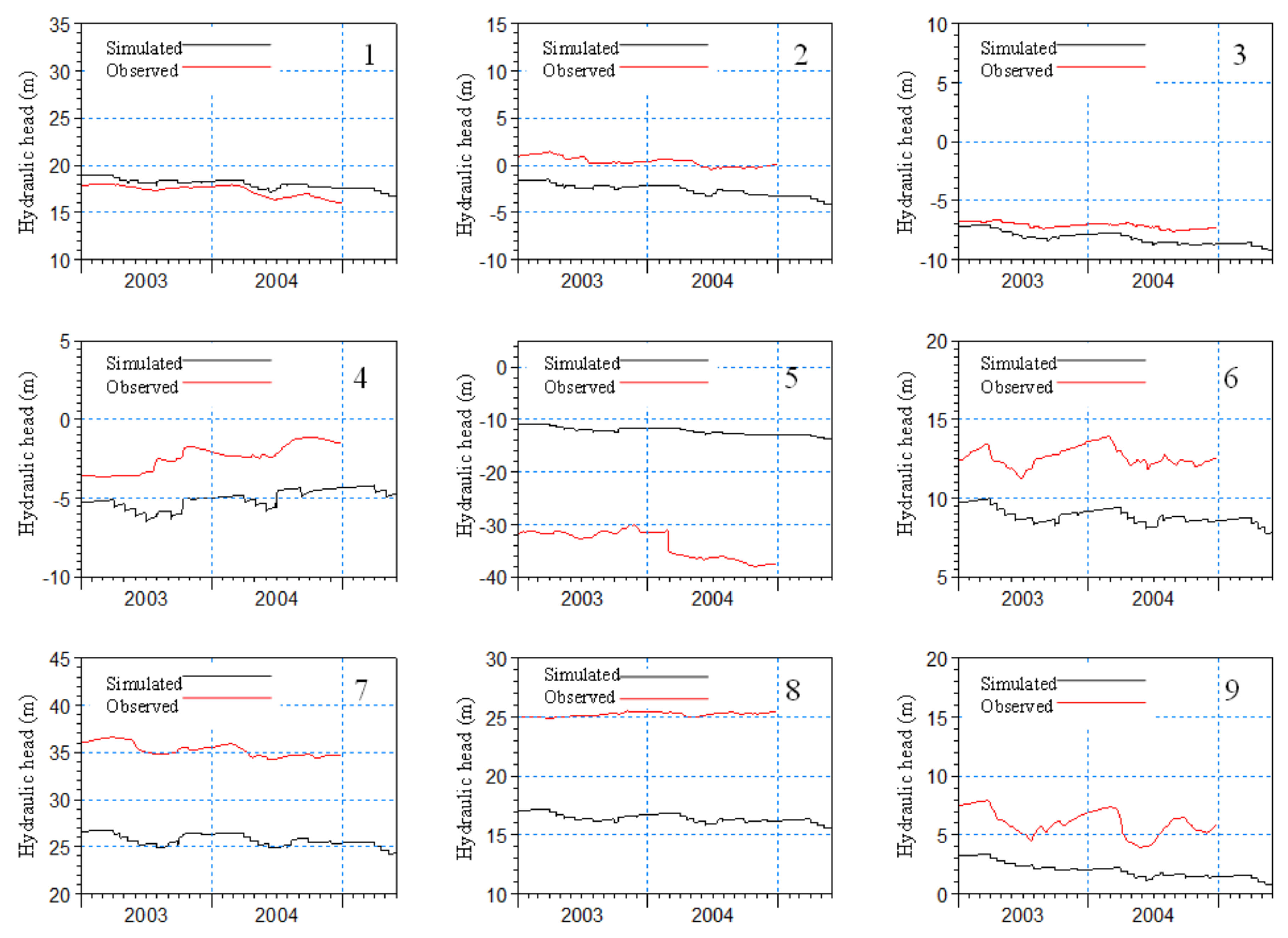
Figure 3 shows examples of the calibration results for nine wells located in different parts of the model area. The graphs highlight the feature in the Haihe Plain that most well exhibit a long-term decline in hydraulic head due to intensive groundwater abstraction for irrigation. The simulations are considered to be in good agreement with observations even though there is an offset in some wells. This is acceptable as long as the overall rate of decline is the same, as discussed above. Figure 4 shows the simulation results for the 2-year validation period for the same wells as in Figure 3. These results further support the reliability of the calibrated hydrological model. The validation process is performed against the surface actual ET from 2003–2007 and groundwater for 2003 and 2004. All the parameters inherit from the calibration optimization results. Good results (Figure 4) from sample 1–5 and 7 are obtained that ME = −1.71, MAE = 1.71, RMSE = 1.76, σ = 0.42, R = 0.83 and Nash_Sutcliffe = −7.9 (sample 1) which is shown in the MIKE SHE output results menu.
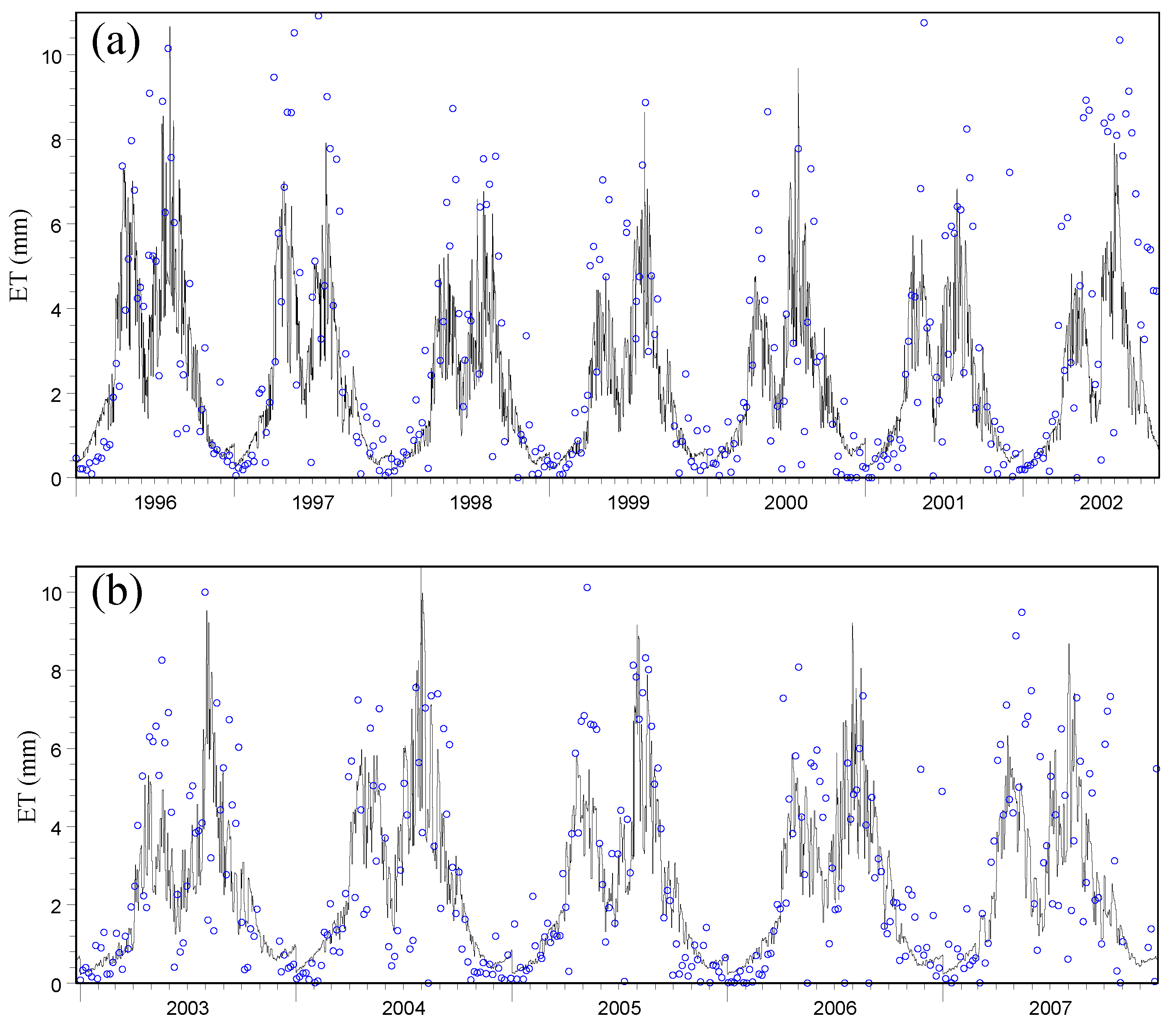
In Figure 5, simulated actual ET by MIKE SHE is compared to measurements from the lysimeter operated at Luancheng experimental station for both the calibration period and the subsequent period (1996–2008). The lysimeter has the same wheat/maize rotation as in the overall region. The parameters determining ET are not considered in the calibration but were adopted from our previous study [4]. As shown by the figure, the model provides a good description of the seasonal dynamics of actual ET, including the double peak, which is a characteristic of the winter wheat-summer maize rotation. However, the levels are not always in agreement particularly during periods with high ET. These differences could be attributed to heat advection influencing the lysimeter measurements and to the fact that the two data sets represent different spatial scales.
2.3. Modelling Based on RS Data
2.3.1. FY-2C Precipitation Products
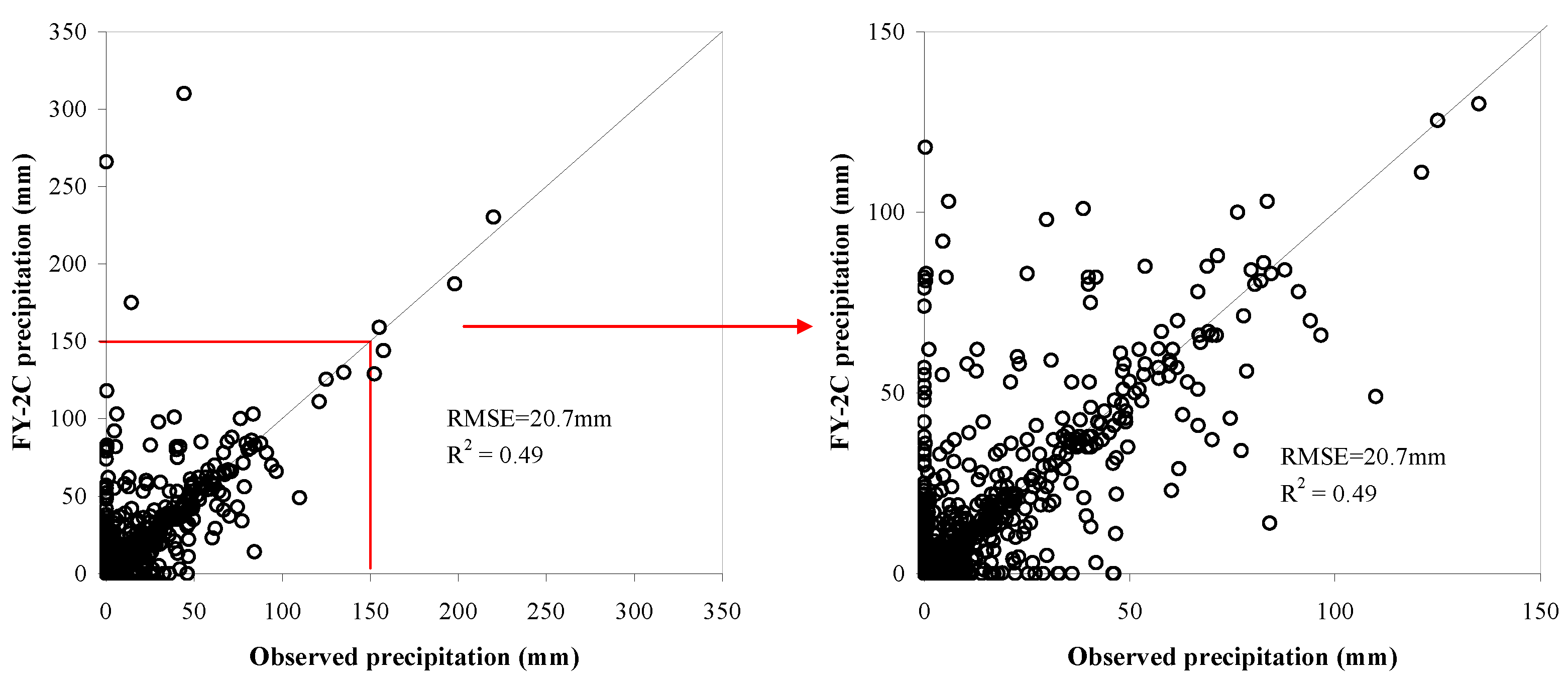
The RS precipitation data applied in this study are a subset of the FY-2C daily precipitation products covering the area of latitude 0°–50° N and longitude 55°–155° E and with a spatial resolution of 0.1° (approximately 11 km) and a temporal resolution of 1 day [38]. Precipitation products were collected for the period June 2005–August 2008. The relative error of the precipitation products applicable for the study region has been estimated to be 30% on a daily basis according to the FY-2C user guide [38]. In Figure 6, we have compared 7-days accumulated precipitation from rain gauges for the period June 2005 to August 2008 (the nine stations within Hebei province) and the FY-2C product (representing the pixel where the rain gauge is located). There are some instances where the FY-2C-based estimates are considerably higher than the ground measurements highlighting that the statistical relations behind the precipitation products are subject to significant uncertainties and thus need to be corrected before being used as a driving variable in the hydrological model.
To improve the quality of the FY-2C precipitation products we applied a correction method that takes the rain gauge measurements as the ground truth while preserving the spatial pattern from RS data as much as possible. The first step is to calculate the overall mean field bias (MFB) between rain gauge observations and the corresponding satellite image pixels:
where G is gauge measurement, PS is estimated rainfall based on remote sensing in the grid cell encompassing the gauge, and N is the number of rain gauges. First, the mean field bias at each remote sensing image is removed by simply multiplying each pixel by the MFB factor:
where n and m are the dimensions of the PS images. After removing the mean field bias, the residual deviations between available G/PS pairs are quantified as:
where Zk is the local rain gauge and remote sensing residual. The next step is to spatially interpolate the residuals by using ordinary kriging.
For the convenience of calculation, point kriging is used:
is the unobserved points in the precipitation field, and λ(i,j) is the linear weights for each G/PS residual. Finally, the corrected PS precipitation is obtained by adding the kriged residual field to the MFB-adjusted RS field:
The following remarks need to be noted when using this method. First of all, if all rain gauges report zero precipitation, it is then considered a dry day. Therefore, should the satellite product give any value, they will be neglected. Second, if the satellite product gives zero precipitation in all pixels and at least one of the gain gauges report a precipitation event, the satellite product will be discarded and the precipitation field is generated by using kriging of station data.
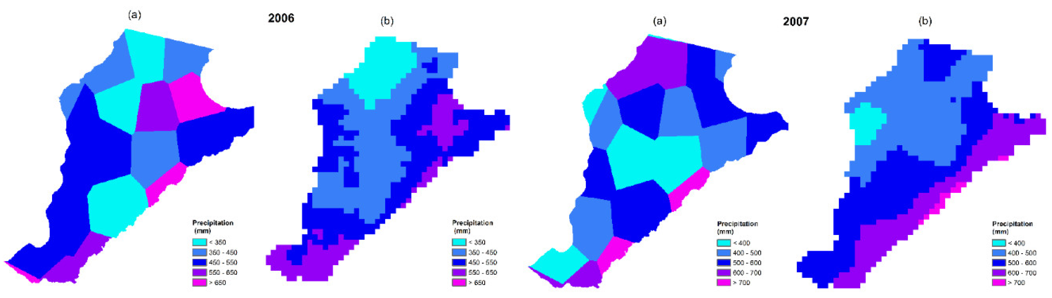
The spatial distributions of annual precipitation of 2006 and 2007, based on conventional and remote sensing data respectively, are shown in Figure 7. When remote sensing data are utilized, a smoother precipitation pattern is introduced as opposed to the Thiessen polygon method, which is characterized by sharp jumps between precipitation zones. The conventional data set might be improved by using kriging interpolation, however, the spatial patterns are also quite different suggesting that the remote sensing data contains additional spatial information to the rain gauge network.
2.3.2. Potential Evapotranspiration
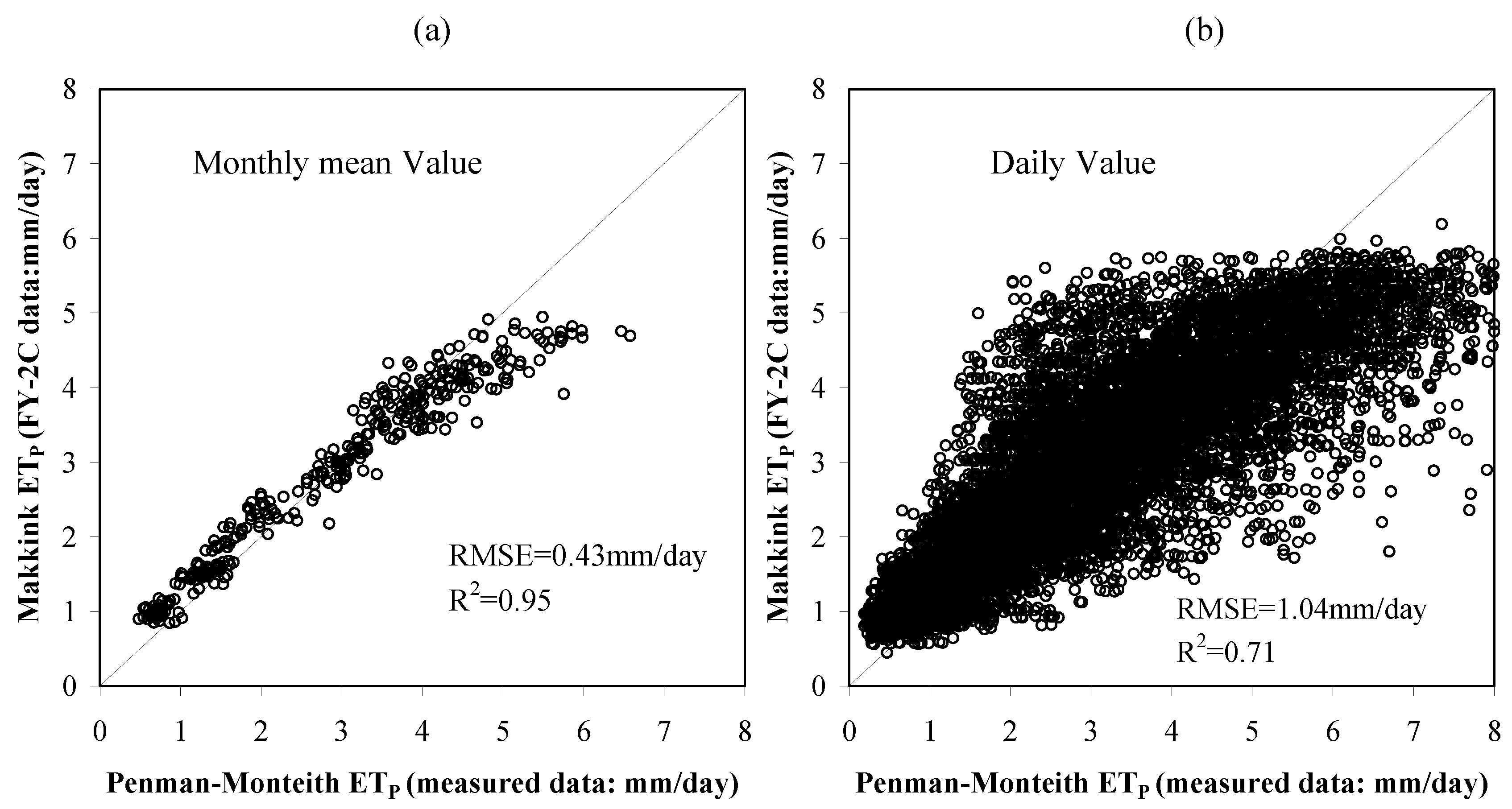
When using RS-driving variables in the model, daily potential evapotranspiration (ETp) is estimated by the Makkink ’s equation [39], which is an empirical regression equation between ETp and incoming solar radiation (Rs) and is based on the assumption that the aerodynamic effects can be neglected. The Makkink formulation is attractive for RS applications because Rs can be estimated from geostationary satellite data.
where Rs is incoming solar radiation (MJ/m2/day), Δ is the slope of saturated vapour pressure curve (kPa/°C), γ is the psychrometric constant (kPa/°C), c1 is an empirical constant which is assumed to be 0.75 [5], and λ is the latent heat of vaporization (MJ/kg). Rs is taken from the FY-2C product, which is based on the DISORT model (Discrete Ordinates Radiative Transfer Program for a Multi-Layered Plan × 10-Parallel Medium) [40,41] using FY-2C cloud products combined with ground observation data. The product for global radiation has an aerial coverage of 60° N–60° S, 45–165° E and a spatial resolution of 1° corresponding to approximately 110 km. The spatial resolution is high compared to the coverage given by the observation data from 98 meteorological stations distributed within China, which can directly monitor the global radiation [38].
In Figure 8, calculations of potential evapotranspiration based on measured standard climate data (Penman-Monteith equation) and RS data (Makkink equation) are compared for the period June 2005 to August 2008 for both monthly values (Figure 8a) and daily values (Figure 8b). For lower ETp rates, acceptable comparisons are obtained, but for higher values it appears that the method based on RS data under-predicts presumably due to the neglect of the aerodynamic term and the scale differences.
The FY-2C precipitation product corrected by the method described previously and potential ET based on the FY-2C product for global radiation were used for driving the hydrological model for the period June 2005–August 2008. Because no measurements of groundwater heads are available for this period, the RS driven model has not been recalibrated. The available ground observation is lysimeter measurements of actual ET until December 2007.
2.4. Comparison of Conventional and RS Models
The overlapping period for the conventional and RS driven models is June 2005 to August 2008, which then allows for a comparison of predicted variables for this period. The comparison of the conventional and RS hydrological Model was carried out in three parts. First, the total water balance for the whole study area from two different models are evaluated to check the impact of each component of total water balance. Second, spatial variations of ET results from these two models are comprised. In this step, daily actual ET maps derived from the FY-2C data combined with MODIS products were used for the evaluation of hydrological model simulations. These daily actual ET maps are based on the improved triangle method [5]. The estimated results have been compared to lysimeter data from the Luancheng field station [4]. Third, spatial variations of groundwater table change were evaluated using the groundwater head difference between the start date (9 June 2005) and the end date (30 August 2008).
3. Results
3.1. Total Water Balance Components
In Table 5, the simulated total water balance components for the model area during 2006 to 2007 from the overlapped time period are listed for the two models using different input data. The results listed in the table provide further documentation of the mining of the groundwater due to pumping for irrigation. Precipitation components derived from FY-2C are significantly larger than the conventional precipitation record in 2006, while both values are very close in 2007. From RS model, we can see that although the total precipitation nearly satisfy the crop water consumption, the irrigation water is still need. That is because the precipitation is seasonally uneven. Irrigation need for the dry winter and spring which is the winter wheat growing season. Since most of small-scale farm households in the Haihe Plain need to turn to use irrigation wells on their scheduled shift, the usual annual change in precipitation has little effect on the regional average irrigation rates little. We set same irrigation rate for 2006 and 2007 and components of pumping in two years had almost same amount. For the model output results in 2006, two components from the RS-model, saturated zone storage change and groundwater recharge, are larger than the conventional model, which is caused by the difference in precipitation. While precipitation is large under the RS model in 2006, groundwater recharge from excess irrigation and rainfall is very significant (Table 5).
3.2. Actual ET
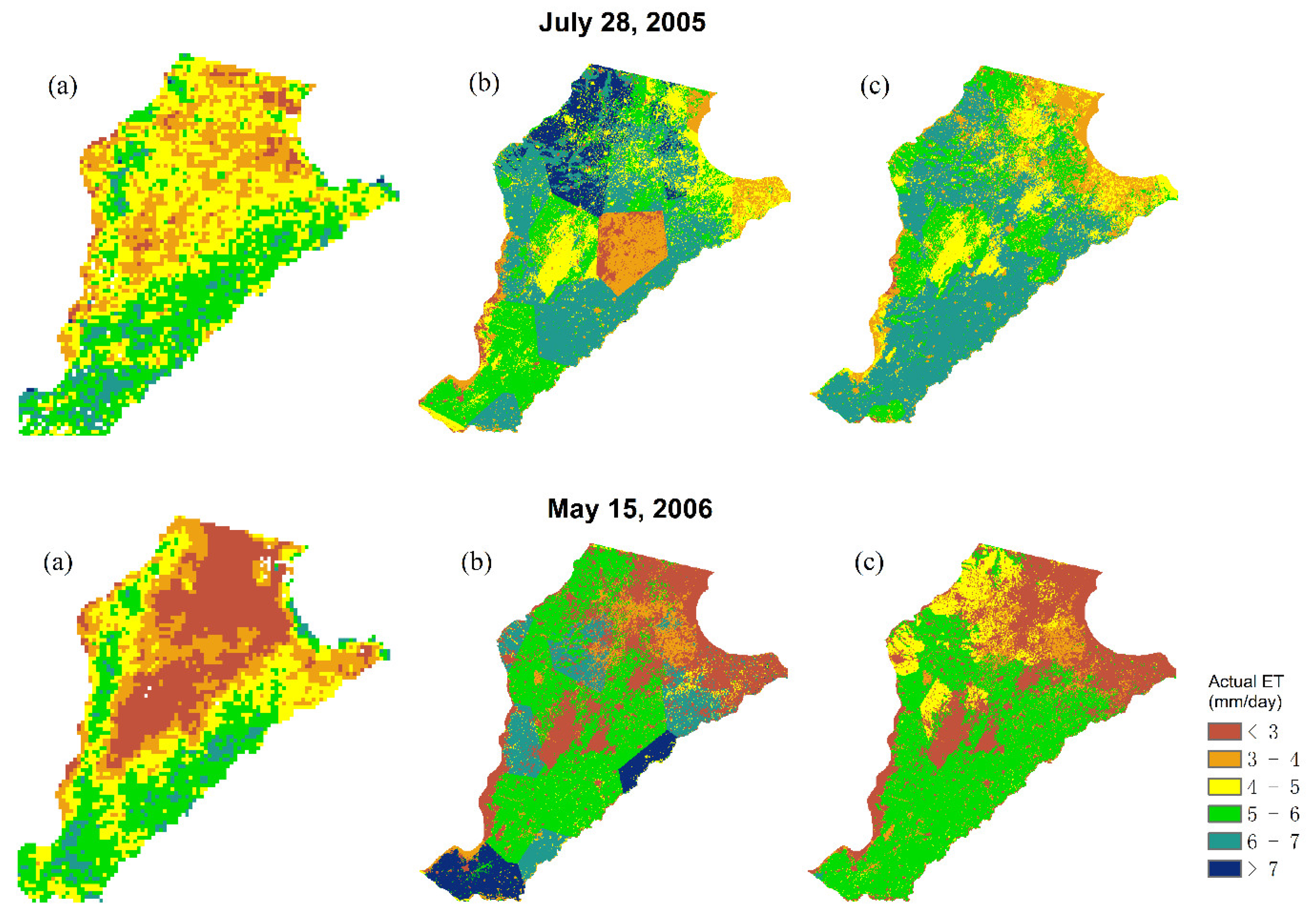
Figure 9 shows the spatial pattern of the daily actual ET on 28 July 2005 and 15 May 2006. Generally, the maps derived directly from the RS-data are more heterogeneous than the results modeled by MIKE SHE. This heterogeneous is caused by the (sub-grid) buildings, trees, windbreaks, biotypes, non-uniform fertilization rate and variation in soil textural and hydraulic parameters [18,42]. RS-ET is simulated based on the energy balance budget regardless of the climate data like precipitation and reference ET. In regard to the RS-ET, the different spatial resolutions of the surface temperature map from FY-2C (5 km) and NDVI from MODIS (1 km) were also found to introduce scatter in the results.
ET predictions by MIKE SHE are controlled by the spatial distribution and resolution of the driving variables (precipitation, reference ET, and irrigation) and parameters (land cover, soil classification, vegetation characteristics, and soil properties). The highest value of daily ET is located in the piedmont of Mt. Taihang and along the edge of the Yellow River where there is normally the highest crop yield of growing winter wheat and summer maize. In the middle and east of the Haihe Plain, the ET value is relatively low where the quality of soil is poor, as there is a large proportion of saline soil [43]. All data based on conventional data sources have a rather coarse spatial resolution. Precipitation and reference ET are specified using Thiessen polygons, which have a characteristic length scale of approximately 80 km in our case. The 25 simulation results reflect the characteristics of Thiessen polygon as well as the pattern of land use classification. This shows that precipitation and ETp as driving parameters and the vegetation classification are critical and sensitive for the simulations. However, compare to ET map calculated triangle methods (Figure 9a), map based on conventional data has a higher spatial resolution (Figure 9b). Precipitation based on FY-2C products has a spatial resolution of about 11 km, which thus adds more spatial variability to the most important driving variable. The map based on RS data (Figure 9c) has a higher spatial variability but its pattern is more similar to the map of Triangle method calculated than the conventional model.
3.3. Groundwater Dynamic Change
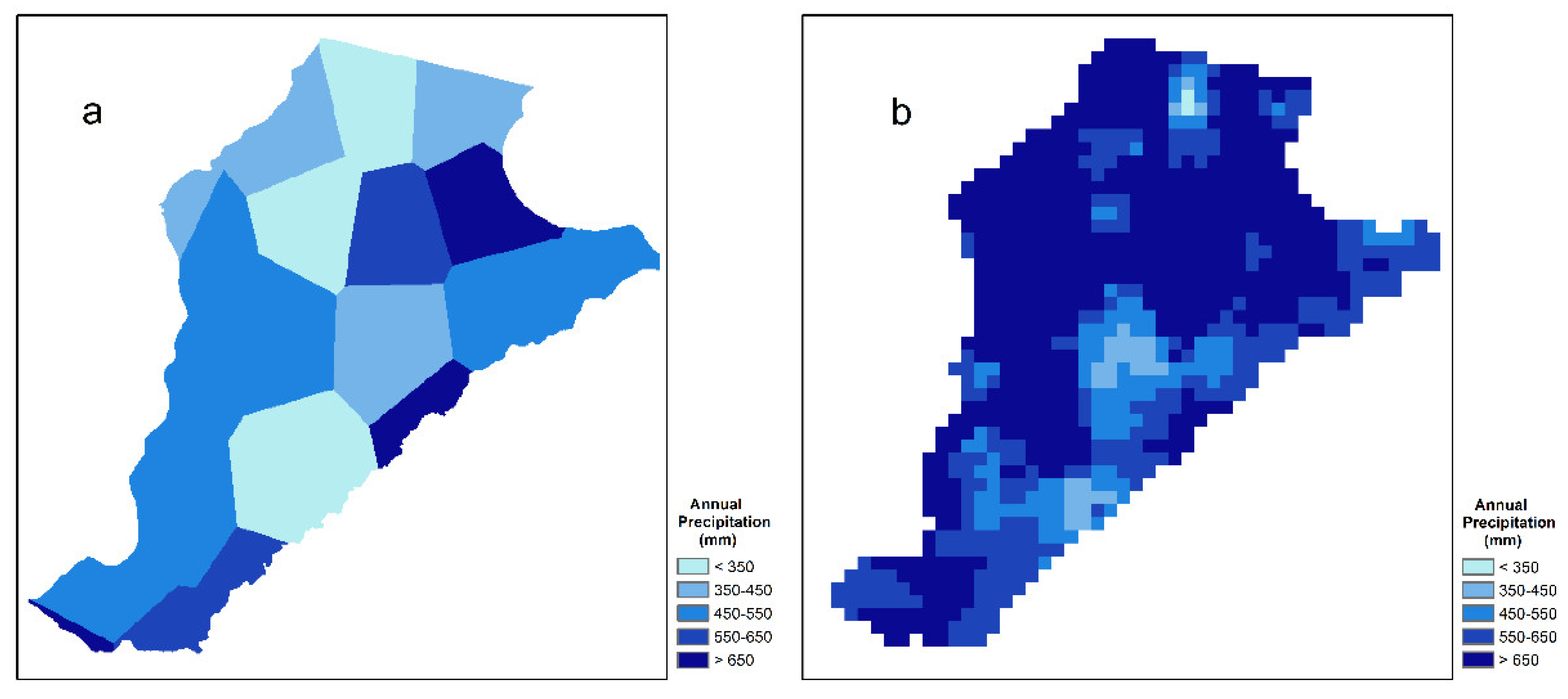
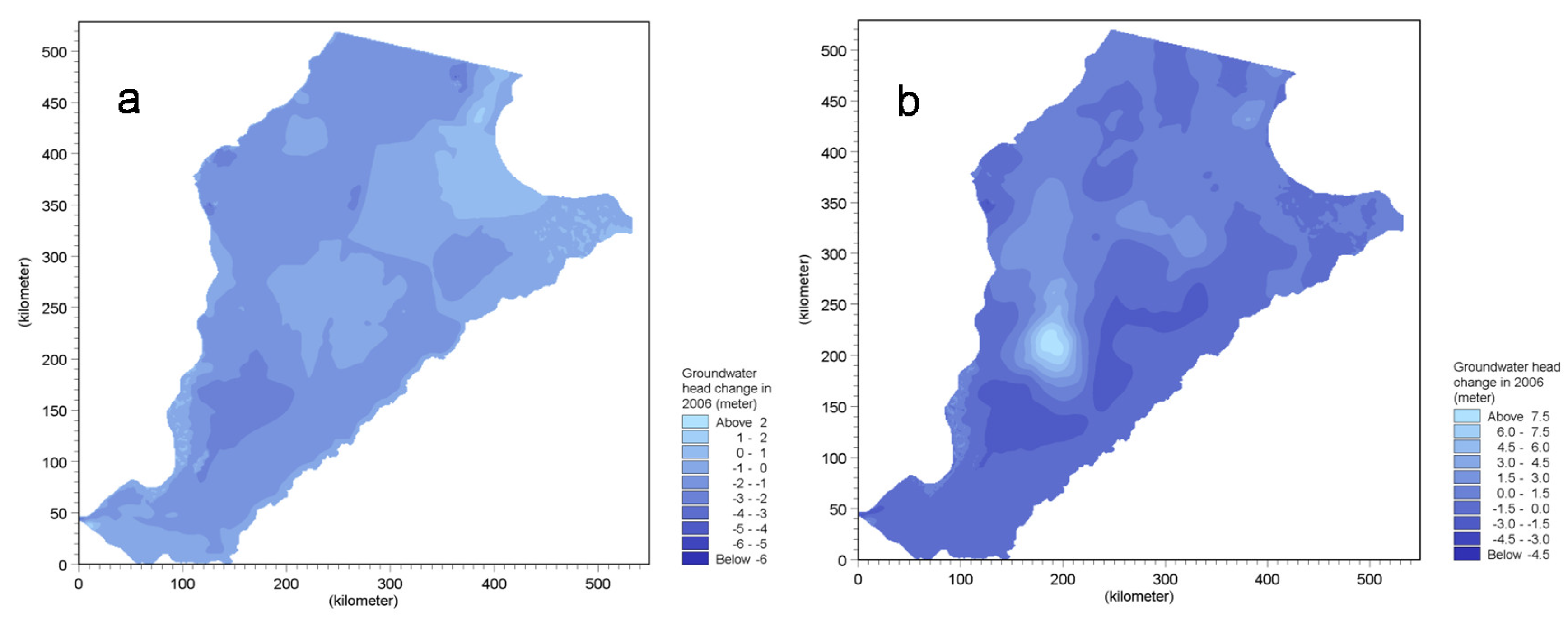
The climate feature of the Haihe Plain is characterized by long periods without precipitation, where the water stored in the unsaturated zone is either recharged to the groundwater or evaporated [24]. During short duration and high intensity of rainfall the conventional actual ET model responds very rapidly due to the increased water content in the root zone and high actual ET rates are simulate in the subsequent periods. As the different precipitation input, these different discrepancy should be exist in the groundwater system respond. The spatially distributed precipitation input based on raingauge data and RS data for 2006, respectively, are shown in Figure 10, which reveals significant difference in the precipitation input in many areas. And this difference also transfer to the groundwater dynamic changes since in the Haihe Plain, the precipitation is the most recharge input for the groundwater system. Figure 11 shows an example from the scatter points: one is the similar precipitation input, and the other is the pronounced higher precipitation in the RS precipitation scenario as compared to the raingauge scenario. And this difference obviously affected the whole groundwater flow distribution. It is evident that the deviations in the precipitation between the two scenarios has imprints the deviations in groundwater elevation.
While irrigation by groundwater is one of the dominating hydrological features (Table 5), the spatial variations of ET reflected the groundwater depletion [4]. The spatial distribution of saturated zone storage change has extreme variation (Figure 11). That implies the vertical recharge from precipitation is vital for groundwater distribution in the Haihe Plain. The distribution of model input data that generate the spatial pattern of water resources on the regional scale will influence the water resource allocation in water management.
4. Discussion
To expand the insight into the hydrology and water resources of the Haihe Plain, we have collected relevant conventional meteorological and hydrological data together with RS products for the area. However, the different types of data were not overlapping in time, which put some constraints on our analysis.
Due to incomplete overlaps in time periods of the relevant data, we only calibrated the hydrological model on the basis of conventional data for a 7-year period. Due to the intensive utilization of the water resources, natural flow in the river systems is virtually absent and, therefore, a traditional calibration of the hydrological model against river discharge observations was not possible and water balance closure will therefore be uncertain. Instead, as irrigation by groundwater is the dominating hydrological feature, the seasonal and spatial variations of ET and groundwater heads are the most relevant calibration targets. Ground observations of ET are only available from one site within this large area and, therefore, calibration of vegetation and soil parameters were not considered in this study, and instead we relied on parameter values determined by Shu et al. [27]. The model was successfully validated against independent groundwater level measurements over 2 years following the calibration period. The model also provided a reasonable match of the lysimeter measurements of ET as far as the seasonal variation is concerned. Since we made the assumption that the calibrated model is applicable for analyzing the effect of using RS products as driving variables, the results of calibration suggest that the calibrated model will provide trustful simulations of the hydrological conditions of the region within the given data constraints.
The comparisons show that precipitation is a critical factor for the hydrological response and for the spatial distribution of the hydrological processes in this model. Traditional rain gauges are not ideally placed in the Haihe Plain and their locations are separated by large distance. Perhaps the absolute amount of rainfall may be captured relatively accurately, but the detailed spatial distribution is not described. This problem is especially serious during the summer time when the weather types are dominated by convective rains where the possibility for a convective storm to fall in between the rain gauges is high. Inaccurate land cover parameterization and irrigation distribution further contribute to the discrepancies.
5. Conclusions
This study demonstrated the potential for modelling groundwater using remote sensing data for deriving important variables for distributed hydrological modelling. An important complication in using RS data for hydrological purposes is that certain types of data are affected by the atmospheric conditions such as cloud cover that may induce several gaps in time. Other data types like precipitation are affected by biases and large errors for certain events. RS precipitation data provide higher spatial distribution, but the raw data is corrupted by unrealistic outliers at certain instances and correction is thus needed. A common method as applied in this study is to merge ground observations and the RS data by forcing the RS data to obey the measurements at the gauge stations and by keeping the RS spatial structure in between. In the Haihe Plain, accurate spatial and temporal ET pattern is very important in the groundwater resource assessment that determines the recharge to the saturated zone. The water consumption of crops in this region can indirectly reflect the groundwater pumping and change distribution since groundwater is the dominating, irrigation resource here. Since actual ET is not able to be measured directly, many methods have been developed; however, uncertainty also goes with them.
This study is the first attempt to apply FY-2C products in groundwater modelling. As the Fengyun geostationary satellite has a very good view angle and coverage for the whole of China, it offers promising perspectives for the application of different products in hydrological assessments and regional water resources management.
Author Contributions
Conceptualization, Y.S. and Y.L.; Methodology, Y.S.; Formal Analysis, Y.S.; Data Collection, Y.L., Y.S. and H.L.; Writing—Original Draft Preparation, Y.S.; Writing—Review & Editing, Y.S. and Y.L.; Funding Acquisition, Y.L. and H.L.
Funding
The work was supported by the National Key Research and Development Program of China (2016YFD0800106), the International Water Management Institute (IWMI), Sri Lanka and Department of Geography and Geology, University of Copenhagen.
Acknowledgments
The authors are grateful to Karsten H. Jensen (University of Copenhagen), Karen G. Villholth (IWMI Southern Africa), Simon Stisen (Geological Survey of Denmark and Greenland), and Inge Sandholt (Technical University of Denmark) for their many constructive suggestions to study and write the draft manuscript. Groundwater data was provided by the Hebei hydrological water resources survey bureau. FY-2C products and weather data were provided China Meteorological Data Service Center.
Conflicts of Interest
The authors declare no conflict of interest.
References
- Kumar, S.; Sekhar, M.; Bandyopadhyay, S. Assimilation of remote sensing and hydrological data using adaptive filtering techniques for watershed modelling. Curr. Sci. 2009, 97, 1196–1202. [Google Scholar]
- Doppler, T.; Honti, M.; Zihlmann, U.; Weisskopf, P.; Stamm, C. Validating a spatially distributed hydrological model with soil morphology data. Hyorol. Earth Syst. Sci. 2014, 18, 3481–3498. [Google Scholar] [CrossRef]
- Frana, A.S. Applicability of Mike She to Simulate Hydrology in Heavily Tile Drained Agricultural Land and Effects of Drainage Characteristics on Hydrology. Master’s Thesis-ProQuest Dissertations & Theses Global, 2012. Available online: http://lib.dr.iastate.edu/cgi/viewcontent.cgi?article=3866& context =etd&httpsredir=1&article=3866&context=etd (accessed on 18 September 2018).
- Shu, Y.; Villholth, K.G.; Jensen, K.H.; Stisen, S.; Lei, Y. Integrated hydrological modeling of the North China plain: Options for sustainable groundwater use in the alluvial plain of MT. Taihang. J. Hydrol. 2012, 464–465, 79–93. [Google Scholar] [CrossRef]
- Stisen, S.; Jensen, K.H.; Sandholt, I.; Grimes, D.I.F. A remote sensing driven distributed hydrological model of the Senegal River basin. J. Hydrol. 2008, 354, 131–148. [Google Scholar] [CrossRef]
- Van Roosmalen, L.; Sonnenborg, T.O.; Jensen, K.H. Impact of climate and land use change on the hydrology of a large-scale agricultural catchment. Water Resour. Res. 2009, 45. [Google Scholar] [CrossRef] [Green Version]
- Qin, H.; Cao, G.; Kristensen, M.; Refsgaard, J.C.; Rasmussen, M.O.; He, X.; Liu, J.; Shu, Y.; Zheng, C. Integrated hydrological modeling of the North China plain and implications for sustainable water management. Hydrol. Earth Syst. Sci. 2013, 17, 3759–3778. [Google Scholar] [CrossRef] [Green Version]
- Beven, K. How far can we go in distributed hydrological modelling? Hydrol. Earth Syst. Sci. 1999, 5, 1–12. [Google Scholar] [CrossRef]
- Refsgaard, J.C. Parameterisation, calibration and validation of distributed hydrological models. J. Hydrol. 1997, 198, 69–97. [Google Scholar] [CrossRef]
- Fu, S.; Sonnenborg, T.O.; Jensen, K.H.; He, X. Impact of precipitation spatial resolution on the hydrological response of an integrated distributed water resources model. Vadose Zone J. 2011, 10, 25–36. [Google Scholar] [CrossRef]
- Bitew, M.M.; Gebremichael, M. Evaluation of satellite rainfall products through hydrologic simulation in a fully distributed hydrologic model. Water Resour. Res. 2011, 47. [Google Scholar] [CrossRef] [Green Version]
- Brunner, P.; Hendricks Franssen, H.J.; Kgotlhang, L.; Bauer-Gottwein, P.; Kinzelbach, W. How can remote sensing contribute in groundwater modeling? Hydrogeol. J. 2006, 15, 5–18. [Google Scholar] [CrossRef]
- Li, H.T.; Brunner, P.; Kinzelbach, W.; Li, W.P.; Dong, X.G. Calibration of a groundwater model using pattern information from remote sensing data. J. Hydrol. 2009, 377, 120–130. [Google Scholar] [CrossRef]
- Milzow, C.; Kgotlhang, L.; Kinzelbach, W.; Meier, P.; Bauer-Gottwein, P. The role of remote sensing in hydrological modelling of the Okavango Delta, Botswana. J. Environ. Manag. 2009, 90, 2252–2260. [Google Scholar] [CrossRef] [PubMed]
- Andersen, J.; Dybkjaer, G.; Jensen, K.H.; Refsgaard, J.C.; Rasmussen, K. Use of remotely sensed precipitation and leaf area index in a distributed hydrological model. J. Hydrol. 2002, 264, 7. [Google Scholar] [CrossRef]
- Fana Biftu, G.; Yew Gan, T. A semi-distributed, physics-based hydrologic model using remotely sensed and digital terrain elevation data for semi-arid catchments. Int. J. Remote Sens. 2004, 25, 4351–4379. [Google Scholar] [CrossRef]
- Diop, M.; Grimes, D.I.F. Satellite-based rainfall estimation for river flow forecasting in Africa. II: African easterly waves, convection and rainfall. Hydrol. Sci. J. 2003, 48, 585–599. [Google Scholar] [CrossRef]
- Boegh, E.; Thorsen, M.; Butts, M.B.; Hansen, S.; Christiansen, J.S.; Abrahamsen, P.; Hasager, C.B.; Jensen, N.O.; van der Keur, P.; Refsgaard, J.C.; et al. Incorporating remote sensing data in physically based distributed agro-hydrological modelling. J. Hydrol. 2004, 287, 279–299. [Google Scholar] [CrossRef]
- Simons, G.; Bastiaanssen, W.; Ngô, L.; Hain, C.; Anderson, M.; Senay, G. Integrating global satellite-derived data products as a pre-analysis for hydrological modelling studies: A case study for the red river basin. Remote Sens. 2016, 8, 279. [Google Scholar] [CrossRef]
- Campo, L.; Caparrini, F.; Castelli, F. Use of multi-platform, multi-temporal remote-sensing data for calibration of a distributed hydrological model: An application in the Arno Basin, Italy. Hydrol. Process. 2006, 20, 2693–2712. [Google Scholar] [CrossRef]
- Immerzeel, W.W.; Droogers, P. Calibration of a distributed hydrological model based on satellite evapotranspiration. J. Hydrol. 2008, 349, 411–424. [Google Scholar] [CrossRef]
- Zhang, Y.; Chiew, F.H.S.; Zhang, L.; Li, H. Use of remotely sensed actual evapotranspiration to improve rainfall–runoff modeling in Southeast Australia. J. Hydrometeorol. 2009, 10, 969–980. [Google Scholar] [CrossRef]
- Liu, J.; Zheng, C.M.; Zheng, L.; Lei, Y.P. Ground water sustainability: Methodology and application to the north china plain. Ground Water 2008, 46, 897–909. [Google Scholar] [CrossRef] [PubMed]
- Shen, H.; Leblanc, M.; Tweed, S.; Liu, W. Groundwater depletion in the Hai river basin, china, from in situ and grace observations. Hydrol. Sci. J. 2015, 60, 671–687. [Google Scholar] [CrossRef]
- Jiang, L.; Islam, S. Estimation of surface evaporation map over southern great plains using remote sensing data. Water Resour. Res. 2001, 37, 329–340. [Google Scholar] [CrossRef]
- Stisen, S.; Sandholt, I.; Nørgaard, A.; Fensholt, R.; Jensen, K.H. Combining the triangle method with thermal inertia to estimate regional evapotranspiration—Applied to msg-seviri data in the senegal river basin. Remote Sens. Environ. 2008, 112, 1242–1255. [Google Scholar] [CrossRef]
- Shu, Y.; Stisen, S.; Jensen, K.H.; Sandholt, I. Estimation of regional evapotranspiration over the North China plain using geostationary satellite data. Int. J. Appl. Earth Obs. Geoinf. 2011, 13, 192–206. [Google Scholar] [CrossRef]
- Moiwo, J.P.; Yang, Y.; Li, H.; Han, S.; Yang, Y. Impact of water resource exploitation on the hydrology and water storage in baiyangdian lake. Hydrol. Process. 2010, 24, 3026–3039. [Google Scholar] [CrossRef]
- Sun, R.; Jin, M.; Giordano, M.; Villholth, K.G. Urban and rural groundwater use in Zhengzhou, China: Challenges in joint management. Hydrogeol. J. 2009, 17, 1495–1506. [Google Scholar] [CrossRef]
- Yan, J.R.S. Keith Simulation of integrated surface water and ground water systems—Model formulation. J. Am. Water Resour. Assoc. 1994, 30, 12. [Google Scholar] [CrossRef]
- Allen, R.G.P.; Raes, D.; Smith, M. Crop Evapotranspiration—Guidelines for Computing Crop Water Requirements—Fao Irrigation and Drainage Paper 56; Food and Agriculture Organization of the United Nations: Rome, Italy, 1998; Available online: http://www.fao.org/docrep/X0490E/x0490e00.htm (accessed on 18 September 2018).
- Xu, J.M. Manual for Fengyun-2 Satellite Products and Satellite Data Format; China Meteorology Press: Beijing, China, 2008. (In Chinese) [Google Scholar]
- CMA. China Meteorological Administration Report on Precipitation Products; the Coordination Group for Meteorological Satellites, China Meteorological Administration, China. 2010. Available online: http://www.eumetsat.int/website/wcm/idc/idcplg?IdcService=GET_FILE&RevisionSelectionMethod=LatestReleased&Rendition=Web&dDocName=CWPT_1539 (accessed on 18 September 2018).
- Cheng, L. Assessment Study of Merged Precipitation and Multiple Satellite Precipitation Products. Master’s Thesis, College of Remote Sensing, Nanjing University of Information Engineering, Nanjing, China, 2013. [Google Scholar]
- Jia, J.; Yu, J.; Liu, C. Groundwater Regime and Calculation of Yield Response in North China Plain: A Case Study of Luancheng County in Hebei Province. J. Geogr. Sci. 2002, 12, 217–225. [Google Scholar]
- Wang, S.; Song, X.; Wang, Q.; Xiao, G.; Liu, C.; Liu, J. Shallow groundwater dynamics in North China plain. J. Geogr. Sci. 2009, 19, 175–188. [Google Scholar] [CrossRef]
- Doherty, J. Pest-Asp User’s Mannual; Scientific Software Group: Provo, UT, USA, 2001. [Google Scholar]
- National Satellite Meteorological Centre. FY-2C Products User Guide; China Meteorological Data Service Center: Beijing, China, 2008. (In Chinese) [Google Scholar]
- Makkink, G.F. Testing the penman formula by means of lysimeters. J. Inst. Water Eng. 1957, 11, 277–288. [Google Scholar]
- Liang, S.; Townshend, J.R. A modified hapke model for soil bidirectional reflectance. Remote Sens. Environ. 1996, 55, 181–189. [Google Scholar] [CrossRef]
- Liang, S.; Lewis, P. A parametric radiative transfer model for sky radiance distribution. J. Quant. Spectrosc. Radiat. Transf. 1996, 55, 9. [Google Scholar] [CrossRef]
- Boegh, E.; Soegaard, H. Remote sensing based estimation of evapotranspiration rates. Int. J. Remote Sens. 2004, 25, 2535–2551. [Google Scholar]
- Wang, S.; Song, X.; Wang, Q.; Xiao, G.; Wang, Z.; Liu, X.; Wang, P. Shallow groundwater dynamics and origin of salinity at two sites in salinated and water-deficient region of North China plain, China. Environ. Earth Sci. 2012, 66, 729–739. [Google Scholar]
Figure 1.
Location of study area. The boundary conditions of the hydrological model for the area are defined as follows: b1: specified gradient along Mt. Taihang ridge, b2: specified gradient at the south-western boundary, b3: specified hydraulic head along the Yellow river, b4: specified hydraulic head (0 m) along the coast line, b5: no-flow along a streamline toward north.

Figure 2.
Maps of land cover, soil type and hydrogeological units. (a) land cover types based on MODIS NDVI of 2003, the black triangles represent points used for actual ET estimation comparison; (b) soil type; (c) hydrogeological units. On the map (c), the white circle marks for the observation wells used auto-calibration and the cross marks for wells exampled in Figure 3 and Figure 4.

Figure 3.
Comparison of observed and simulated hydraulic heads for selected wells (calibration period).
Figure 3.
Comparison of observed and simulated hydraulic heads for selected wells (calibration period).

Figure 4.
Comparison of observed and simulated hydraulic heads for selected wells (validation period).
Figure 4.
Comparison of observed and simulated hydraulic heads for selected wells (validation period).

Figure 5.
Time series of ET modeled by MIKESHE (full line) are compared to the observed evapotranspiration value (blue circle) in the calibration period (a) and validation period (b).
Figure 5.
Time series of ET modeled by MIKESHE (full line) are compared to the observed evapotranspiration value (blue circle) in the calibration period (a) and validation period (b).

Figure 6.
Comparison of weekly measured precipitation by rain gauges and estimates from FY-2C data of original data for nine stations within Hebei Province.
Figure 6.
Comparison of weekly measured precipitation by rain gauges and estimates from FY-2C data of original data for nine stations within Hebei Province.

Figure 7.
Spatial distribution of annual precipitation (mm) for year 2006 and 2007. (a) rain gauge measurements (Thiessen polygons); (b) based on remote sensing products which has been corrected.
Figure 7.
Spatial distribution of annual precipitation (mm) for year 2006 and 2007. (a) rain gauge measurements (Thiessen polygons); (b) based on remote sensing products which has been corrected.

Figure 8.
Comparison of ETp calculated by the Penman-Monteith equation on the basis of measured meteorological data and the Makkink equation based on the FY-2C incoming solar radiation product. (a) monthly mean values, (b) daily mean values for the period June 2005 to August 2008.
Figure 8.
Comparison of ETp calculated by the Penman-Monteith equation on the basis of measured meteorological data and the Makkink equation based on the FY-2C incoming solar radiation product. (a) monthly mean values, (b) daily mean values for the period June 2005 to August 2008.

Figure 9.
Daily actual ET maps for 2 days: 28 July 2005 and 15 May 2006. (a) triangle method, (b) model based on conventional data, (c) model based on RS.
Figure 9.
Daily actual ET maps for 2 days: 28 July 2005 and 15 May 2006. (a) triangle method, (b) model based on conventional data, (c) model based on RS.

Figure 10.
Spatial distribution of annual precipitation of Haihe Plain in 2006 (a) using precipitation based on rain gauge data; (b) using precipitation based on RS data.
Figure 10.
Spatial distribution of annual precipitation of Haihe Plain in 2006 (a) using precipitation based on rain gauge data; (b) using precipitation based on RS data.

Figure 11.
Spatial distribution of groundwater head change in 2006 (a) using precipitation data based on rain gauge data; (b) calculated based on RS data.
Figure 11.
Spatial distribution of groundwater head change in 2006 (a) using precipitation data based on rain gauge data; (b) calculated based on RS data.


Table 1.
Maps and time series used as input to MIKE SHE with reference to the source and the spatial discretization.
Table 1.
Maps and time series used as input to MIKE SHE with reference to the source and the spatial discretization.
| Date Type | Date Resource | Spatial Discretisation |
|---|---|---|
| Distributed maps | ||
| Topography/DEM | SRTM 90 m Digital Elevation Data (http://srtm.csi.cgiar.org/) | 90 × 90 m |
| Landscape (vegetation) | MODIS NDVI based classification | 250 × 250 m |
| Soil types | Soil map of Hebei province | |
| Precipitation zones | Stations distributed by Thiessens Polygon Method | 23 points |
| Potential evapotranspiration zones | Stations distributed by Thiessens Polygon Method | 23 points |
| Initial groundwater head | Interpolation from observed groundwater heads | 200 heads |
| Bottom elevation of the aquifer system | Hebei Geological map | 1:500,000 |
| Geological units | Huanghuaihai Plain geology map | |
| RS precipitation products | FY-2C products | 0.1° × 0.1° |
| RS potential evapotranspiration | FY-2C products | 1° × 1 ° |
| Time series | ||
| Precipitation | National meteorological stations | |
| Potential evapotranspiration | National meteorological stations | |
| LAI | Measured or from reference | |
| Kc | Measured or from reference | |
| Root depth | Measured or from reference |
Table 2.
Soil hydraulic parameterization of the two-layer model for the unsaturated zone.
| Soil Type | θsat | θfc | θwp | Ks (m/s) |
|---|---|---|---|---|
| Loam | 0.47 | 0.386 | 0.102 | 5.2 × 10⁻⁶ |
| Sandy | 0.43 | 0.1 | 0.05 | 1 × 10⁻³ |
| Sandy loam | 0.41 | 0.35 | 0.07 | 8 × 10⁻⁶ |
| Clay loam | 0.42 | 0.39 | 0.14 | 3.5 × 10⁻⁸ |
Table 3.
Parameters chosen for calibration.
| Parameters * | Initial Value | Parameter Ties | Lower Bound | Upper Bound | Final Value |
|---|---|---|---|---|---|
| K1 (m/s) | 0.004 | tied to K2 | 1.00 × 10⁻¹⁰ | 1.00 × 10¹⁰ | 0.0037 |
| Sy1 | 0.25 | tied to Sy2 | 1.00 × 10⁻¹⁰ | 1.00 × 10¹⁰ | 0.266 |
| K2 (m/s) | 0.002 | 1.00 × 10⁻¹⁰ | 1.00 × 10¹⁰ | 0.0018 | |
| Sy2 | 0.2 | 1.00 × 10⁻¹⁰ | 1.00 × 10¹⁰ | 0.212 | |
| K3 (m/s) | 0.001 | tied to K4 | 1.00 × 10⁻¹⁰ | 1.00 × 10¹⁰ | 0.0010 |
| Sy3 | 0.153 | tied to Sy4 | 1.00 × 10⁻¹⁰ | 1.00 × 10¹⁰ | 0.20 |
| K4 (m/s) | 0.001 | 1.00 × 10⁻¹⁰ | 1.00 × 10¹⁰ | 0.0010 | |
| Sy4 | 0.15 | 1.00 × 10⁻¹⁰ | 1.00 × 10¹⁰ | 0.196 | |
| K5 (m/s) | 0.0005 | tied to K6 | 1.00 × 10⁻¹⁰ | 1.00 × 10¹⁰ | 0.0006 |
| Sy5 | 0.1 | tied to Sy6 | 1.00 × 10⁻¹⁰ | 1.00 × 10¹⁰ | 0.135 |
| K6 (m/s) | 0.0002 | 1.00 × 10⁻¹⁰ | 1.00 × 10¹⁰ | 0.0002 | |
| Sy6 | 0.08 | 1.00 × 10⁻¹⁰ | 1.00 × 10¹⁰ | 0.108 | |
| b1 | 0.0015 | 1.00 × 10⁻¹⁰ | 1.00 × 10¹⁰ | 0.0010 | |
| b2 | 0.0015 | 1.00 × 10⁻¹⁰ | 1.00 × 10¹⁰ | 0.0012 |
K represents the horizontal saturated hydraulic conductivity; K1, K2, K3, K4, K5 and K6 refer to the horizontal saturated hydraulic conductivity in Unit 1, Unit 2, Unit 3, Unit 4, Unit 5 and Unit 6, respectively. Sy represents the specific yield; Sy1, Sy2, Sy3, Sy4, Sy5 and Sy6 refer to the specific yield for Unit 1, Unit 2, Unit 3, Unit 4, Unit 5 and Unit 6, respectively. b1 and b2 refer to the upstream boundary conditions shown in Figure 1.
Table 4.
Statistic of the objective function for the calibration.
| Statistic | Daily | 5-Day | ||||
|---|---|---|---|---|---|---|
| RMSE | dherror | ab(dherror) | RMSE | dherror | ab(dherror) | |
| Max | 19.77 | 15.67 | 15.67 | 36.01 | 11.31 | 15.02 |
| Min | 0.79 | −6.76 | 0.01 | 0.57 | −15.02 | 0.02 |
| Mean | 6.21 | 0.08 | 3.63 | 8.92 | 0.06 | 3.28 |
| σ | 4.87 | 4.98 | 3.41 | 7.16 | 4.23 | 2.67 |
Table 5.
Simulated water balance components in 2006 and 2007 (Unit: mm/year).
| Water Balance Components | 2006 | 2007 | ||
|---|---|---|---|---|
| Conventional Model | RS Model | Conventional Model | RS Model | |
| Precipitation | 456 | 742 | 524 | 533 |
| Actual evapotranspiration | 673 | 769 | 698 | 726 |
| Unsaturated zone storage change | −7 | −22 | 27 | 19 |
| Saturated zone storage change | −193 | 12 | −182 | −193 |
| Pumping for irrigation | 271 | 271 | 270 | 271 |
| Pumping for industry and domestic use | 5 | 5 | 5 | 5 |
| Groundwater recharge | 64 | 269 | 71 | 60 |
| Lateral inflow | 25 | 25 | 27 | 27 |
| Lateral outflow | 1 | 1 | 1 | 4 |
© 2018 by the authors. Licensee MDPI, Basel, Switzerland. This article is an open access article distributed under the terms and conditions of the Creative Commons Attribution (CC BY) license (http://creativecommons.org/licenses/by/4.0/).
Share and Cite
MDPI and ACS Style
Shu, Y.; Li, H.; Lei, Y. Modelling Groundwater Flow with MIKE SHE Using Conventional Climate Data and Satellite Data as Model Forcing in Haihe Plain, China. Water 2018, 10, 1295. https://doi.org/10.3390/w10101295
AMA Style
Shu Y, Li H, Lei Y. Modelling Groundwater Flow with MIKE SHE Using Conventional Climate Data and Satellite Data as Model Forcing in Haihe Plain, China. Water. 2018; 10(10):1295. https://doi.org/10.3390/w10101295
Chicago/Turabian StyleShu, Yunqiao, Hongjun Li, and Yuping Lei. 2018. "Modelling Groundwater Flow with MIKE SHE Using Conventional Climate Data and Satellite Data as Model Forcing in Haihe Plain, China" Water 10, no. 10: 1295. https://doi.org/10.3390/w10101295
Note that from the first issue of 2016, this journal uses article numbers instead of page numbers. See further details here.