Identifying the Sensitivity of Ensemble Streamflow Prediction by Artificial Intelligence

Abstract

Sustainable water resources management is facing a rigorous challenge due to global climate change. Nowadays, improving streamflow predictions based on uneven precipitation is an important task. The main purpose of this study is to integrate the ensemble technique concept into artificial neural networks for reducing model uncertainty in hourly streamflow predictions. The ensemble streamflow predictions are built following two steps: (1) Generating the ensemble members through disturbance of initial weights, data resampling, and alteration of model structure; (2) consolidating the model outputs through the arithmetic average, stacking, and Bayesian model average. This study investigates various ensemble strategies on two study sites, where the watershed size and hydrological conditions are different. The results help to realize whether the ensemble methods are sensitive to hydrological or physiographical conditions. Additionally, the applicability and availability of the ensemble strategies can be easily evaluated in this study. Among various ensemble strategies, the best ESP is produced by the combination of boosting (data resampling) and Bayesian model average. The results demonstrate that the ensemble neural networks greatly improved the accuracy of streamflow predictions as compared to a single neural network, and the improvement made by the ensemble neural network is about 19–37% and 20–30% in Longquan Creek and Jinhua River watersheds, respectively, for 1–3 h ahead streamflow prediction. Moreover, the results obtained from different ensemble strategies are quite consistent in both watersheds, indicating that the ensemble strategies are insensitive to hydrological and physiographical factors. Finally, the output intervals of ensemble streamflow prediction may also reflect the possible peak flow, which is valuable information for flood prevention.

1. Introduction

The frequency and intensity of extreme rainfall events have significantly increased due to climate change in past years. Heavy rainfall is the major cause of flood disasters; therefore, there is an urgent need to construct reliable flood prediction models. Due to special geographical and climatic conditions, the Zhejiang province, China, has always been a flood disaster-prone area. Thus, strategies to effectively deal with flood threats have become a priority. Since the influence of global climate change has become increasingly significant, the former balance of rainfall–runoff mechanisms is failing. The occurrence and intensity of extreme hydrological events are more frequent than those in previous years. To reduce the impact of flood hazards, the development of hydrological prediction models is necessary and urgently required.

Artificial neural networks (ANNs) have been widely used in solving a wide range of hydrological problems, such as rainfall–runoff modeling [1,2], regional flood frequency analysis [3], groundwater modeling [4,5,6,7], hydrological time series modeling, and reservoir operation [8,9]. Hydrological prediction models based on ANNs can effectively identify the relationship between the input and output in hydrological systems, which can overcome the weaknesses of the conventional method of parameterized modeling. For complex rainfall–runoff modeling, ANNs can also produce reliable outputs through historical data learning. Thus, ANNs have become popular and are generally applied in streamflow predictions over the past decade to lessen flood-induced damage.

However, the uncertainty of ANNs comes from several factors, such as the selection of input variables, model structures, initial weights, and calibration data [10,11]. One way to reduce the ANNs’ uncertainty is to integrate the ensemble technique into ANN models. Research in the field of ensemble streamflow predictions (ESP) has been remarkably increasing in order to avoid model errors due to single deterministic results of hydrological prediction [12,13]. Nowadays, ensemble prediction has developed into multimode, multianalysis prediction techniques, which consider the models’ uncertainty at the initial state and from mode architecture [14]. Because of the flexible geometry of ANNs, they have been recognized as feasible models for ensemble techniques [15].

Tiwari and Chatterjee [16] developed hourly water level forecasting models using bootstrap based ANNs (BANN). Their results indicated that BANN-hydrologic forecasting models with confidence bounds can improve their reliability for flood forecasts. Kasiviswanathan et al. [17] constructed a prediction interval for ANN rainfall runoff models based on ensemble simulations, which showed that generated ensembles predict the peak flow with less error, and most of their observed flows fall within the constructed prediction interval. To forecast urban water demand, a new hybrid wavelet–bootstrap-neural network model was built and performed more accurate forecasting than the traditional neural network, bootstrap-based neural networks, ARIMA (autoregressive integrated moving average), and ARIMAX (autoregressive integrated moving average model with exogenous input variables) models [18]. Ensemble neural network models have also been successfully applied in potential evapotranspiration prediction [19], probabilistic prediction of local precipitation [20], and short-term forecasting of groundwater levels [21].

While many studies have applied ensemble techniques to the hydrologic field, there is still a shortage of studies about the sensitivity of ESP. In this paper, the main objective is to integrate the ensemble technique concept into ANNs, hereafter termed ensemble neural networks (ENNs), for reducing the uncertainty in streamflow predictions. ENNs are then applied to two watersheds with different area and hydrological conditions to discuss the sensitivity on ESP. Four methods are used for generating the ensemble members, and three methods are selected to combine the outputs of ensemble members. A total of twelve ensemble strategies are built separately in two different watersheds to validate if the best ESP is consistent and if the best ensemble combination is sensitive to hydrological and physiographical changes. The methodologies of the artificial neural network and two resampling techniques, stacking average, and Bayesian model average, are briefly described in the following section. The study area and hydrological data are provided in Section 3. Section 4 shows the results and comparison of twelve ESP models and the sensitivity analysis of two watersheds. Finally, the conclusions are given in Section 5.

2. Methodology

This study aims at integrating the ensemble technique concept into ANNs for constructing accurate ensemble streamflow prediction models and identifying both spatial and hydrological sensitivity of ensemble strategies at two distinct watersheds. The related methods are presented as follow.

2.1. Back Propagation Neural Network

The basic concept of artificial neural networks is to simulate the information processing system of biological neural networks by imitating the human nervous system with computer hardware and software. ANNs are composed of many nonlinear operation units, neurons, and links located between the arithmetic units, which usually compute in parallel and dispersedly. The ANNs can be trained through information (data) importing. In this study, the back-propagation neural network (BPNN) [22] is used to construct the streamflow prediction model. The model architecture is shown in Figure 1. The hyperbolic tangent sigmoid transfer function (‘tansig’ in Matlab) and linear transfer function (‘purelin’ in Matlab) are used as the activation functions in hidden and output layers, respectively. The number of neurons in the hidden layer is four, which was determined by trial and error. The rainfall and streamflow at the current and previous time step are used as input variables, and the predicted streamflow is the model output. The BPNN applies the steepest descent method to adjust the weights for minimizing the output error. In the learning process, the weights are adjusted by an error convergence technique to obtain the desired output for a given input dataset.

2.2. Ensemble Neural Network

The ENN is introduced by integrating the ensemble technique concept into neural networks. The principle of the ensemble method is to construct several specific groups with different model outputs (i.e., a collection of members) to predict a certain target (streamflow in this study), and the difference of each model output provides the probability distribution information of the prediction target. As mentioned above, previous research on artificial neural networks showed that the uncertainty can be classified into three parts: Uncertainties of data, uncertainties of initial values, and uncertainties of the model structure (including the parameters of the model). The ensemble technique has been developed to consider the uncertainties of several sources to avoid network error existing in a single predicted result.

In general, the construction of ENNs can be divided into two steps: Generating ensemble members and integrating the outputs obtained from ensemble members. Methods to generate ensemble members in this study include the disturbance of the initial value, the resampling of the training dataset (Bagging resampling and Boosting resampling), and the alteration of model structure (number of neurons in the hidden layer). The methods selected for combining the outputs of ensemble members include arithmetic averaging, the Bayesian model averaging [15,23], and stack averaging. Another important issue is related to the number of ensemble members. According to Chiang et al. [24], the suggested number of ensemble members used for hydrological forecasting is twenty, which is based on a compromise between output accuracy and computational time. Their recommendation holds for different model types and model structures (i.e., conceptual models and neural networks). Thus, twenty ensemble members were used in this study.

2.3. Generating Ensemble Members

As mentioned, the model uncertainty mainly comes from initial values, model structures, and data. Thus, ensemble member generation focuses on reducing these uncertainties. First, a single neural network (SNN), which only uses a calibrated single back-propagation neural network, is generally given random initial values when calibrating the model structure and model parameters. However, ENN in this study starts from a plurality of random initial weights, computes the local optimum value, and extracts useful information to increase the probability of accurate predictions. Subjected to the influence of random initial values, the results obtained may vary in each calibration. Therefore, each network model is trained several times to minimize error of the objective function, which can be regarded as a local optimization. This procedure is repeated 20 times to obtain 20 ensemble members with different initial weights.

Uncertainty from the ANN model structure mainly comes from the number of hidden neurons, since the input and output dimension was fixed in this study. Because the number of ensemble member is 20, the number of hidden neurons from 1 to 20 is assigned to the 20 ensemble members in sequence by using the model structure alternating strategy (ENN4, ENN8, and ENN 12 in

Table 1. Combinations of ensemble neural networks.

		Integrating Member
		Arithmetic Average	Bayesian Model Average	Stacking Average
Generating member	Disturbance of initial value	ENN1	ENN5	ENN9
	Bagging resampling skill	ENN2	ENN6	ENN10
	Boosting resampling skill	ENN3	ENN7	ENN11
	Alteration of model structure	ENN4	ENN8	ENN12

). For example, the hidden neuron for ensemble member 1 is 1, the hidden neuron for ensemble member 2 is 2, and so on. The remaining two strategies of generating members used the best number of hidden neuron, which is the same as the single BPNN (four neurons).

As for the uncertainty of training data, a common method to eliminate its influence is the resampling technique, in which the samples are selected from the original amount of data according to certain rules for enhancing the amount of training sample. The resampling methods applied in this study are the bagging resampling algorithm and boosting resampling algorithm.

The bagging method is proposed for obtaining an aggregated predictor from multiple generated datasets of individual predictors [25]. The assumption of this method is that, given a standard training dataset T of size N, the distribution probability of each element of the training data is uniform, that is, 1/N. Then, the training dataset of a member network, TB, is generated by sampling by replacing N times from the original training dataset T using these probabilities. This process is repeated, and each member of a neural network is generated with a different random sampling, assigned from the original training set.

The boosting algorithm is a method for reducing bias and variance in machine learning and can improve model performance by producing a series of predictors trained with a different distribution of the original training data. The algorithm trains the first member of the neural network with the original training set, and the training dataset of a new member of the neural networks is assigned based on the performance of the previous member of the ensemble. The learning processes in which predicted values produced by the previous member differ significantly from their observations are adjusted with higher probability of being sampled. In this case, these data will have a higher chance to exist in the new training dataset than those correctly predicted, and therefore different members of ensemble are specialized in different parts of the observation space. There are many boosting algorithms, and the procedure of the second version of ADABoost was used in this study [26].

2.4. Integrating Ensemble Members

2.4.1. Arithmetic Averaging

Arithmetic averaging is the simplest averaging method and a popular method for the ensemble technique to combine the models’ outputs. Generally, combination using single averaging is defined as:

$$\overline{\mathrm{y}}=\frac{1}{K}{\displaystyle \sum _{k=1}^K{y}_i^k},i=1,2,\dots ,N$$

(1)

where K represents the number of ensemble members, y represents output, and N represents the total number of data points.

2.4.2. Stack Averaging

In general, stacking is not a specific algorithm but a generic name [27]. It means that, when training on part of the training dataset, the performance of the learning machine on the training dataset was not part of the training set for that particular machine giving additional information [28]. The main procedure of stacking is to combine the networks by tuning their weights over the feature space. The outputs obtained from a set of level 0 generalizers (ensemble members) are fed to level 1 generalizer, which is trained to produce appropriate output. The stacking algorithm was developed by Breiman [29], who suggested minimizing the following function:

$$W={\displaystyle \sum _{i=1}^m[x_i-{\displaystyle \sum _{k=1}^N{c}_k}{\widehat{x}}_i^k],c_k>0}$$

(2)

The stacked average produces estimates for the coefficients c₁, c₂, …, c_k, which are used to construct the ensemble prediction:

$${\widehat{x}}_i={\displaystyle \sum }_{k=1}^N{c}_k{\widehat{x}}_i^k, i=1,2,\dots ,m$$

(3)

Equation (3) minimizes squared absolute differences between observations and predictions. This process could be dominated by those patterns with large errors when it is used to calculate the coefficients. A better choice, as adopted in this study, is to minimize the squared relative difference:

$$H={\displaystyle \sum _{i=1}^m(\frac{x_i-{\displaystyle \sum _{k=1}^N{c}_k{\widehat{x}}_i^k}}{x_i}){}^2},c_k>0$$

(4)

2.4.3. Bayesian Model Average

The Bayesian model average (BMA) is capable of obtaining reliable overall predictive values through calculating different weights for all selected models [30,31,32]. The probability density function of prediction y based on BMA is as follows:

$$p\left(y|D\right)={\displaystyle \sum _{k=1}^{K}p\left(f_k|D\right)}\cdot p_k\left(y|f_k,D\right)$$

(5)

where $p(f_k|D)$ represents the posterior probability of the k-th neural network model prediction trained by observed data D. In fact, $p(f_k|D)$ is equal to the k-th model $f_k$ corresponding to weights $w_k$, which is larger when the model performance is better, and ${\displaystyle {\displaystyle \sum }_{k=1}^K{w}_k=1, w_k>0}$. $p_k(y|f_k,D)$ represents the posterior distribution of prediction y in neural network model $f_k$ and data D. The posterior distribution of the mean and variance BMA analogic variables can be expressed as:

$$E(y|D)={\displaystyle \sum }_{k=1}^{K}p(f_k|D)\cdot E\left[p_k(y|f_k,D)\right]={\displaystyle \sum }_{k=1}^K{w}_k{f}_k$$

(6)

$$Var(y|D)={\displaystyle \sum }_{k=1}^K{w}_k{\left(f_k-{\displaystyle \sum }_{k=1}^K{w}_k{f}_k\right)}^2+{\displaystyle \sum }_{k=1}^K{w}_k{\sigma }_k^2$$

(7)

where ${\sigma }_k^2$ is the variance of analogic variables under the conditions of observed data D and model $f_k$. Essentially, BMA is the weight of the k-th neural network model’s weighted average. The variance of analogic variables includes error between models and within models. In Equation (7), ${\displaystyle {\displaystyle \sum }_{k=1}^K{\left(f_k-{\displaystyle \sum }_{k=1}^K{w}_k{f}_k\right)}^2}$ is the error between models, and ${\displaystyle {\displaystyle \sum }_{k=1}^K{w}_k{\sigma }_k^2}$ is the error within models.

3. Applications

The BPNN was used in building the single and ensemble forecasting models. As for the ensemble scenario, there were a total of twelve ENN models that are implemented for ESP, and these ENN models were derived from the combinations of four generating methods and three combination skills. Detailed information is displayed in Table 1.

3.1. Study Area and Data Description

Longquan Creek is the source of the Oujiang River, which is the second largest river in the Zhejiang province in China (Figure 2). In Figure 2, the triangle represents the watershed outlet and the circles represent the rain gauge locations. Longquan Creek flows to the East sea of China, with a drainage area of 1440 km² and length of 160 km. The watershed receives an annual rainfall of about 1807 mm, and more than 80% of rainfall comes from the monsoon period (from April to June). The hydrological features of Longquan Creek are rapid streamflow and short period of flood peak, due to uneven distribution of rainfall and mountainous topography. This results in the Longquan Creek watershed being a flood-prone area.

The Jinhua River is the largest tributary of the Qiantang River, which is the largest river in the Zhejiang province (Figure 2). The Jinhua River flows to the East sea of China, with a drainage area of approximately 6781 km² and length of 200 km. Jinhua River watershed is located in a subtropical climate zone. The rainwater of this watershed mainly comes from typhoons. The watershed receives an annual rainfall of approximately 1450 mm. Due to the characteristics of typhoon rainfall (high intensity in a short duration), Jinhua River watershed is also a flood-prone area.

These two watersheds were selected in this study to determine if the ensemble strategies are sensitive to hydrological and physiographical factors. The differences between Longquan Creek and the Jinhua River watershed can be summarized as follow: (1) The watersheds have different shapes and sizes; (2) the rainfall type is monsoon and typhoon rainfall, respectively, and (3) Longquan Creek is located in a mountainous area (upstream) and the Jinhua River is located in a midstream, flat area. Two types of data, hourly streamflow (Q) and average hourly rainfall (P), were used as input variables to build ensemble streamflow predictions in this study. This study used the Pearson correlation coefficient [33] to find the high correlation input variables. The time-dependent variables Q(t), Q(t − 1), Q(t − 2), and P(t − 3), where t is the current time, were selected in the Longquan Creek basin, and Q(t), Q(t − 1), Q(t − 2) and P(t − 10) were selected in the Jinhua River basin.

A total of 37 flood events occurred in Longquan Creek, and 70 flood events occurred in the Jinhua River during the collection period of 1994 to 2013. Even though the number of events is different, the sample sizes are sufficient to train the neural networks in both watersheds. The arrangement of data in training, validation, and testing phases follows the ratio of 3:1:1.

Table 2. The statistics of streamflow in three datasets (m³/s).

Statistic	Longquan Creek			Jinhua River
	Training	Validation	Testing	Training	Validation	Testing
Max.	3040	2430	2640	4200	3810	3640
Min.	13	7	11	2	6	3
Mean	248	216	202	514	575	510
STD	323	318	256	550	628	528

shows the statistics of streamflow measurements in three independent datasets. The statistics includes maximum, minimum, mean, and standard deviation (STD) of streamflow.

3.2. Evaluation Criteria

The coefficient of determination (R²), root mean square error (RMSE), and G_bench index (G_bench) were used in this study to evaluate the accuracy of a single neural network and ensemble neural network.

(i)

Coefficient of Determination (R²)

$$R^2=1-\frac{{\displaystyle \sum _{t=1}^N{\left(Q_{obs}\left(t+n\right)-Q_{pre}\left(t+n\right)\right)}^2}}{{\displaystyle {\displaystyle \sum }_{t=1}^N{\left(Q_{obs}\left(t+n\right)-{\overline{Q}}_{obs}\right)}^2}}$$

(8)

where $Q_{obs}\left(t+n\right)$ and $Q_{pre}\left(t+n\right)$ are the observed and predicted flow at time t + n, ${\overline{Q}}_{obs}\left(t\right)$ is the mean of the observed runoff, and N is the number of data points. The value of R² varies between negative infinity and one. Values approaching one indicate higher accuracy in model performance.

(ii)

root mean square error (RMSE)

$$\mathrm{RMSE}=\sqrt{\frac{{\displaystyle {\displaystyle \sum }_{t=1}^N{\left(Q_{obs}\left(t+n\right)-Q_{pre}\left(t+n\right)\right)}^2}}{N}}$$

(9)

The merits of models can be significantly reflected through RMSE values when assessing peak values of variables.

(iii)

G_bench index (G_bench)

$$G_{bench}=1-\frac{{\displaystyle {\displaystyle \sum }_{t=1}^N{\left(Q_{pre}\left(t+n\right)-Q_{obs}\left(t+n\right)\right)}^2}}{{\displaystyle {\displaystyle \sum }_{t=1}^N{\left(Q_{obs}\left(t+n\right)-Q_{bench}\left(t\right)\right)}^2}}$$

(10)

where $Q_{bench}\left(t\right)$ represents the benchmark series of real observed runoff at time t. G_bench is negative if the model performance is poorer than the benchmark, zero if the model performs as well as the benchmark, and positive if the model is superior. Values closer to one indicate a perfect fit [34].

4. Results and Discussions

In this study, the single BPNN was calibrated using the training dataset, and the validation dataset was applied to check the overfitting issue. Then, the twelve ensemble strategies were integrated into BPNN models to build the ensemble streamflow predictions. Results obtained from SNN and ENNs in both watersheds are described below, as well as the comparison of model accuracy and the sensitivity of ensemble strategies.

4.1. Comparison of a Single Neural Network and Ensemble Neural Network

Table 3. Testing results obtained from the single neural network (SNN) and 12 ensemble neural networks (ENNs) in the Longquan Creek watershed.

Criteria	R2			RMSE			Gbench
Lead Time	1 h	2 h	3 h	1 h	2 h	3 h	1 h	2 h	3 h
SNN	0.984	0.955	0.928	32.2	54.3	69.0	0.375	0.489	0.587
ENN1	0.993	0.976	0.945	21.9	39.4	60.0	0.712	0.731	0.688
ENN2	0.993	0.977	0.947	21.6	38.8	59.3	0.720	0.740	0.696
ENN3	0.993	0.976	0.945	21.6	39.8	60.3	0.720	0.726	0.685
ENN4	0.993	0.978	0.944	21.6	38.2	60.7	0.720	0.746	0.680
ENN5	0.993	0.976	0.946	21.7	39.5	59.8	0.718	0.730	0.690
ENN6	0.993	0.979	0.950	21.4	37.4	57.5	0.726	0.757	0.713
ENN7	0.994	0.980	0.953	20.2	36.0	55.6	0.754	0.775	0.732
ENN8	0.993	0.975	0.936	21.8	40.2	65.3	0.715	0.719	0.631
ENN9	0.993	0.976	0.943	21.6	39.5	61.3	0.720	0.730	0.674
ENN10	0.991	0.976	0.950	23.8	40.0	57.7	0.659	0.723	0.711
ENN11	0.990	0.979	0.949	25.8	37.3	57.8	0.600	0.759	0.711
ENN12	0.993	0.971	0.928	22.1	43.8	69.0	0.706	0.668	0.587

shows the test results of forecasted streamflow for 1–3 h lead time in Longquan Creek watershed by the SNN and twelve ENN models. In general, the results produced by all ensemble models are better than the single network model. Among various ensemble strategies, the combination of boosting and BMA (ENN7) provided about 19–37% improvement in terms of RMSE at different lead times compared to the single model. The overall performance of ENN7 was better than other ensemble strategies for 1–3 h ahead streamflow predictions. Compared to other ENN models, the ENN7 model has a higher R², lower RMSE, and higher G_bench, indicating that the combination of the boosting algorithm and Bayesian model average is more reliable for streamflow predictions. Additionally, according to the comparison of the evaluation criteria (Table 3), it can be seen that the single artificial neural network was capable of producing accurate streamflow predictions with the coefficient of determination (R²) being higher than 0.9 for 1–3 h ahead streamflow predictions. In addition, the use of the ensemble technique effectively increased the output accuracy, which means the integration of the ensemble technique and ANN provides a better option for hydrological predictions.

Table 4. Testing results obtained from the SNN and 12 ENNs in the Jinhua River watershed.

Criteria	R2			RMSE			Gbench
Lead Time	1 h	2 h	3 h	1 h	2 h	3 h	1 h	2 h	3 h
SNN	0.996	0.990	0.980	32.3	53.1	75.5	0.827	0.776	0.730
ENN1	0.998	0.993	0.986	23.0	43.3	62.1	0.913	0.851	0.817
ENN2	0.998	0.994	0.987	23.3	42.1	61.1	0.910	0.859	0.823
ENN3	0.998	0.993	0.986	25.9	44.2	62.1	0.888	0.845	0.817
ENN4	0.998	0.992	0.986	23.3	46.0	63.8	0.910	0.832	0.807
ENN5	0.998	0.993	0.987	23.1	42.9	61.8	0.912	0.854	0.819
ENN6	0.998	0.994	0.987	23.5	42.0	60.8	0.909	0.860	0.825
ENN7	0.998	0.994	0.987	22.6	41.8	60.3	0.915	0.862	0.828
ENN8	0.998	0.993	0.985	23.2	44.5	64.0	0.911	0.843	0.806
ENN9	0.998	0.993	0.986	22.7	43.0	62.9	0.915	0.853	0.813
ENN10	0.998	0.994	0.986	23.1	42.5	62.1	0.912	0.857	0.817
ENN11	0.998	0.994	0.987	23.2	42.0	61.1	0.910	0.860	0.823
ENN12	0.998	0.993	0.985	24.2	45.4	64.7	0.903	0.836	0.802

lists the results of the testing dataset obtained from the SNN and twelve ENN models in the Jinhua River watershed. Similar to those by the Longquan Creek watershed, the results produced by ENN models are better than those of the single model. Among various ensemble strategies, the ENN7 model still provided the best performance compared to other ENN models in terms of higher R², lower RMSE, and higher G_bench values. Even though the performance of all ENN models is similar at a lead time of one hour, the results have significant difference as the lead time increases. Compared to the SNN, the improvement made by the ENN7 model is about 20–30% for 1–3 h ahead streamflow predictions in terms of RMSE. The results also demonstrate that the combination of the boosting algorithm and Bayesian model average had a better predictive capability for long-term streamflow predictions. Figure 3 and Figure 4 show the scatterplot of observations and predictions produced by the SNN and ENN7 models in the Longquan Creek and Jinhua River watershed, respectively. It is obvious that the performance obtained from the ENN7 model is much better than that of the SNN model in both watersheds. According to Table 3 and Table 4 and Figure 3 and Figure 4, an important result can be found, which is that the best ensemble strategy (the combination of member generalization and member integration) is neither sensitive to hydrological nor physiographical conditions in terms of streamflow prediction. Therefore, the boosting resampling algorithm is suggested for generating ensemble members and the Bayesian model average is recommended for integrating the outputs of ensemble members.

4.2. Peak Flow Prediction

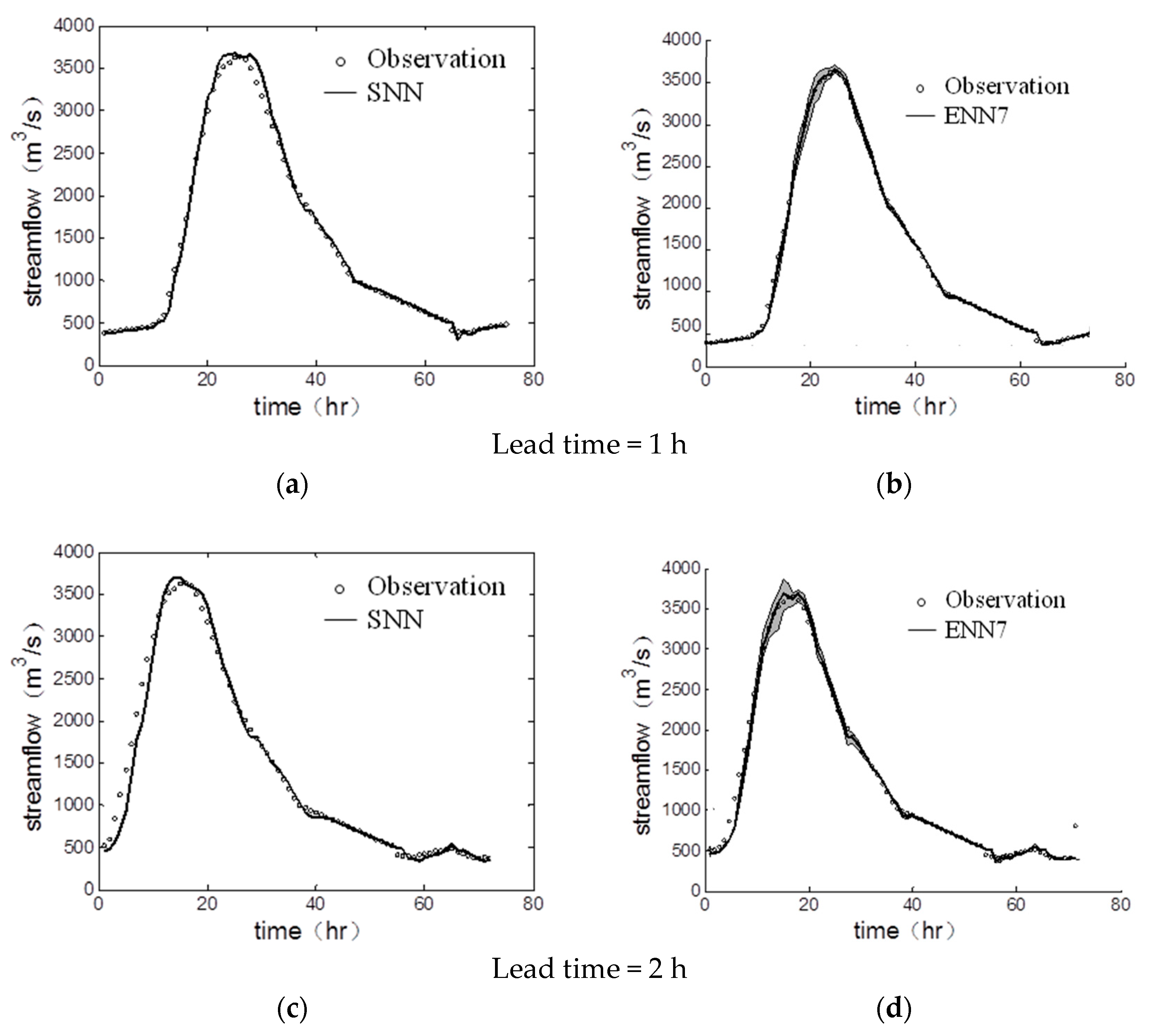
The most important mission is to accurately predict peak flow. Compared to the deterministic prediction from the single model, the ensemble models provide the probabilistic outputs to reduce the uncertainty of model predictions. Figure 5 and Figure 6 illustrate the comparison between SNN and ENN7 models for the largest peak flow during the testing phase in the Longquan Creek and Jinhua River watershed, respectively. In Figure 5 and Figure 6, the circles represent the actual streamflow, the grey area represents the predictive interval consisting of twenty ensemble members, and the black line represents the model prediction. Generally, both SNN and ENN7 models produced reliable predictions for the lead time of one hour in both watersheds. However, as the lead time increases, the predictive hydrograph produced by SNN has a significant time-lag problem, which may result in the failure of flood warning or flood prevention. The predictive hydrograph obtained from ENN7 has much better predictions, and the time-lag problem is insignificant. Furthermore, the SNN underestimated the streamflow in the rising limb and overestimated the streamflow in the recession limb for 2 h and 3 h lead time in both watersheds. On the other hand, the outputs of ENN7 fit the observations well and the predictive interval produced by twenty ensemble members covers almost the whole of the actual streamflow, indicating the ENN7 model maintained robust predictive capability for 2 h and 3 h ahead streamflow prediction. In Figure 5 and Figure 6, it is seen that most of the observed peak flow is covered by the predictive interval (gray area). In the other words, this demonstrates that ENN can effectively reduce the quantitative uncertainty of hydrologic models [35,36].

Based on the presented results, it is found that the model accuracy in the Jinhua River watershed is slightly better than that in the Longquan Creek watershed. This is mainly because the Longquan Creek watershed is located upstream, where the flow velocity is much higher than that in midstream and downstream. Thus, further analysis of peak flow prediction must be discussed.

Table 5. Peak flow prediction produced by ENN7 in both watersheds.

ENN7		Lead Time = 1 h		Lead Time = 2 h		Lead Time = 3 h
	Qp	Qp’ (m3/s)	Error (%)	Qp’ (m3/s)	Error (%)	Qp’ (m3/s)	Error (%)
	Longquan Creek Basin
Event 1	1191	1215	2	1261	6	1181	−0.8
Event 2	2640	2618	−0.8	2510	−5	2466	−6.5
Event 3	1410	1403	−0.5	1524	8	1280	−9
	Jinhua River Basin
Event 1	2520	2523	0.1	2507	−0.5	2508	−0.5
Event 2	3040	3062	0.7	3045	0.2	3165	4.1
Event 3	3640	3665	0.7	3611	−0.8	3731	2.5

Qp: Actual peak flow; Qp’: Forecasted peak flow.

displays the peak flow predictions obtained from the ENN7 model on the first three largest flood events from the testing dataset in both watersheds. The relative error of model predictions in the Longquan Creek watershed and the Jinhua River watershed are within 10% and 5%, respectively, for 1–3 h ahead streamflow prediction, suggesting that the ENN model was able to produce reliable peak flow predictions.

4.3. Sensitivity of Ensemble Neural Networks

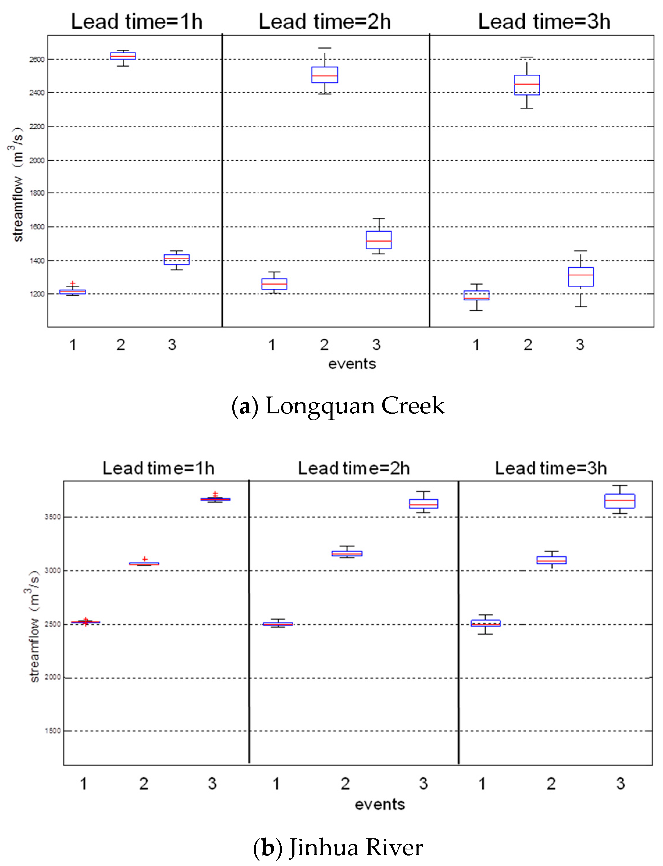
To understand whether the ensemble models are sensitive to hydrological and physiographical conditions, Figure 7 and Figure 8 show the peak flow predictions of the three largest events and the RMSE of the testing dataset at the two watersheds, respectively. It is clear from the boxplot (Figure 7) that the peak flow predictions of twelve ENN models are quite stable and consistent for 1–3 h ahead prediction. Figure 8 indicates the overall performance of twelve ENN models in the testing phase. In general, longer lead time may cause larger bias of model output (larger RMSE value when lead time = 3 h, see Figure 8). However, for the streamflow prediction, the results still show a consistent trend of the twelve ENN models in both watersheds for 1–3 h ahead prediction, in which the ENN7 has the lowest RMSE in both the Longquan Creek and Jinhua River watershed. This result demonstrates that the ESP with the combination of the boosting resampling algorithm (generating member) and Bayesian model average (integrating member) was better than others. Figure 8 also shows the trends of RMSE values of the 12 ENNs in both watersheds. There are three ensemble combinations with different trends of RMSE values in both watersheds (ENN3 and ENN11 when lead time = 1 h, ENN4 when lead time = 2 h). The results indicate that RMSE values depend on ensemble combinations. However, the figure demonstrates that there are similar trends (9 of 12 are similar) in both watersheds (lower sensitivity of ensemble neural networks). In summary, the results displayed in Figure 7 and Figure 8 also indicate the ENN models not only present a higher accuracy of predictive capability, but also reveal their lower sensitivity in ESP.

5. Conclusions

Streamflow prediction is critical for assessing imminent flood risk and evaluating and planning flood mitigation activities. In general, uncertainty and sensitivity are two important considerations in hydrological modeling. The main purpose of this study was to integrate the ensemble technique concept into artificial neural networks to reduce uncertainty and discuss the sensitivity in streamflow predictions. The results show that the ENNs were able to effectively reduce the uncertainty in hydrological modeling, compared to the SNN. Additionally, the best ensemble strategy was identified through both case studies as the combination of boosting resampling and Bayesian model average. The main achievements and innovations of this study are concluded as follows: (1) The ENN models greatly improved the accuracy of streamflow prediction compared to SNN models for 1–3 h ahead prediction in both watersheds. The improvement made by the ENNs is about 20% to 40% in terms of RMSE; (2) the relative error of peak flow predictions in both the Longquan Creek and Jinhua River watershed obtained from the ENN7 model demonstrates that the ensemble model is capable of reflecting the possible maximum flood, which is a valuable reference for flood prevention; (3) the best ensemble strategy integrated into the ANN-based hydrological models in two study watersheds is the same, indicating that the ensemble strategy has low sensitivity to the hydrological and physiographical factors. In other words, the artificial neural network combined with ensemble technique can be applicable for generating streamflow predictions in different flood-prone areas.

References

- Chang, F.J.; Tsai, M.J. A nonlinear spatio-temporal lumping of radar rainfall for modeling multi-step-ahead inflow forecasts by data-driven techniques. J. Hydrol. 2016, 535, 256–269. [Google Scholar] [CrossRef]
- Chokmani, K.; Ouarda, T.; Hamilton, S. Comparison of ice-affected streamflow estimates computed using artificial neural networks and multiple regression techniques. J. Hydrol. 2008, 349, 383–396. [Google Scholar] [CrossRef]
- Shu, C.; Ouarda, T.B.M.J. Flood frequency analysis at ungauged sites using artificial neural networks in canonical correlation analysis physiographic space. Water Resour. Res. 2007, 43, W07438. [Google Scholar] [CrossRef]
- Gong, Y.; Zhang, Y.; Lan, S.; Wang, H. A Comparative Study of Artificial Neural Networks, Support Vector Machines and Adaptive Neuro Fuzzy Inference System for Forecasting Groundwater Levels near Lake Okeechobee, Florida. Water Resour. Manag. 2016, 30, 375–391. [Google Scholar] [CrossRef]
- Maiti, S.; Tiwari, R.K. A comparative study of artificial neural networks, Bayesian neural networks and adaptive neuro-fuzzy inference system in groundwater level prediction. Environ. Earth Sci. 2014, 71, 3147–3160. [Google Scholar] [CrossRef]
- Sreekanth, J.; Datta, B. Stochastic and Robust Multi-Objective Optimal Management of Pumping from Coastal Aquifers Under Parameter Uncertainty. Water Resour. Manag. 2014, 28, 2005–2019. [Google Scholar] [CrossRef]
- Tsai, W.P.; Chiang, Y.M.; Huang, J.L.; Chang, F.J. Exploring the Mechanism of Surface and Ground Water through Data-Driven Techniques with Sensitivity Analysis for Water Resources Management. Water Resour. Manag. 2016, 30, 4789–4806. [Google Scholar] [CrossRef]
- Tsai, W.P.; Chang, F.J.; Chang, L.C.; Herricks, E.E. AI techniques for optimizing multi-objective reservoir operation upon human and riverine ecosystem demands. J. Hydrol. 2015, 530, 634–644. [Google Scholar] [CrossRef]
- Yin, X.A.; Yang, Z.F.; Petts, G.E.; Kondolf, G.M. A reservoir operating method for riverine ecosystem protection, reservoir sedimentation control and water supply. J. Hydrol. 2014, 512, 379–387. [Google Scholar] [CrossRef]
- Deolia, V.K.; Purwar, S.; Sharma, T.N. Stabilization of Unknown Nonlinear Discrete-Time Delay Systems Based on Neural Network. Intell. Control Autom. 2012, 3, 337–345. [Google Scholar] [CrossRef]
- Goyal, V.; Deolia, V.K.; Sharma, T.N. Neural network based sliding mode control for uncertain discrete-time nonlinear systems with time-varying delay. Int. J. Comput. Intell. Res. 2016, 12, 125–138. [Google Scholar]
- Dechant, C.M.; Moradkhani, H. Improving the characterization of initial condition for ensemble streamflow prediction using data assimilation. Hydrol. Earth Syst. Sci. 2011, 15, 3399–3410. [Google Scholar] [CrossRef] [Green Version]
- Faber, B.A.; Stedinger, J.R. Reservoir optimization using sampling SDP with ensemble streamflow prediction (ESP) forecasts. J. Hydrol. 2001, 249, 113–133. [Google Scholar] [CrossRef]
- Hao, Z.; Hao, F.; Singh, V.P. A general framework for multivariate multi-index drought prediction based on Multivariate Ensemble Streamflow Prediction (MESP). J. Hydrol. 2016, 539, 1–10. [Google Scholar] [CrossRef]
- Araghinejad, S.; Azmi, M.; Kholghi, M. Application of artificial neural network ensembles in probabilistic hydrological forecasting. J. Hydrol. 2011, 407, 94–104. [Google Scholar] [CrossRef]
- Tiwari, M.K.; Chatterjee, C. Uncertainty assessment and ensemble flood forecasting using bootstrap based artificial neural networks (BANNs). J. Hydrol. 2010, 382, 20–33. [Google Scholar] [CrossRef]
- Kasiviswanathan, K.S.; Cibin, R.; Sudheer, K.P.; Chaubey, I. Constructing prediction interval for artificial neural network rainfall runoff models based on ensemble simulations. J. Hydrol. 2013, 499, 275–288. [Google Scholar] [CrossRef]
- Tiwari, M.K.; Adamowski, J. Urban water demand forecasting and uncertainty assessment using ensemble wavelet-bootstrap-neural network models. Water Resour. Res. 2013, 49, 6486–6507. [Google Scholar] [CrossRef] [Green Version]
- El-Shafie, A.; Najah, A.; Alsulami, H.M.; Jahanbani, H. Optimized Neural Network Prediction Model for Potential Evapotranspiration Utilizing Ensemble Procedure. Water Resour. Manag. 2014, 28, 947–967. [Google Scholar] [CrossRef]
- Ohba, M.; Kadokura, S.; Yoshida, Y.; Nohara, D.; Toyoda, Y. Downscaling medium-range ensemble forecasts using a neural network approach. Proc. Int. Assoc. Hydrol. Sci. 2015, 369, 7–11. [Google Scholar] [CrossRef] [Green Version]
- Khalil, B.; Broda, S.; Adamowski, J.; Ozga-Zielinski, B.; Donohoe, A. Short-term forecasting of groundwater levels under conditions of mine-tailings recharge using wavelet ensemble neural network models. Hydrogeol. J. 2015, 23, 121–141. [Google Scholar] [CrossRef]
- Rumelhart, D.E. Learning Internal Representations by Error Propagation; MIT Press: Cambridge, MA, USA, 1986; ISBN 0-262-68053-X. [Google Scholar]
- Ouarda, T.B.M.J.; Shu, C. Regional low-flow frequency analysis using single and ensemble artificial neural networks. Water Resour. Res. 2009, 45, 114–122. [Google Scholar] [CrossRef]
- Chiang, Y.M.; Hao, R.N.; Ho, H.C.; Chang, T.J.; Xu, Y.P. Evaluating the contribution of multi-model combination to streamflow hindcasting by empirical and conceptual models. Hydrol. Sci. J. 2017, 62, 1456–1468. [Google Scholar] [CrossRef]
- Breiman, L. Bagging predictors. Mach. Learn. 1996, 24, 123–140. [Google Scholar] [CrossRef] [Green Version]
- Freund, Y.; Schapire, R.E. Experiments with a New Boosting Algorithm. In Proceedings of the Thirteenth International Conference on Machine Learning, Bari, Italy, 3–6 July 1996; pp. 148–156. [Google Scholar]
- Wolpert, D.H. Stacked generalization. Neural Netw. 1992, 5, 241–259. [Google Scholar] [CrossRef] [Green Version]
- Drucker, H. Improving Regressors using Boosting Techniques. In Proceedings of the Fourteenth International Conference on Machine Learning, Nashville, TN, USA, 8–12 July 1997; pp. 107–115. [Google Scholar]
- Breiman, L. Stacked regressions. Mach. Learn. 1996, 24, 49–64. [Google Scholar] [CrossRef] [Green Version]
- Hoeting, J.A.; Madigan, D.M.; Raftery, A.E.; Volinsky, C.T. Bayesian model averaging: A tutorial (with discussion). Stat. Sci. 1999, 14, 382–401. [Google Scholar]
- Kass, R.E.; Raftery, A.E. Bayes factors. J. Am. Stat. Assoc. 1995, 90, 773–795. [Google Scholar] [CrossRef]
- Leamer, E.E. Specification Searches: Ad Hoc Inference with Nonexperimental Data; Wiley: New York, NY, USA, 1978; p. 370. ISBN 978-0471015208. [Google Scholar]
- Pearson, K. Notes on regression and inheritance in the case of two parents. Proc. R. Soc. Lond. 1895, 58, 240–242. [Google Scholar] [CrossRef]
- Seibert, J. On the need for benchmarks in hydrological modelling. Hydrol. Process. 2001, 15, 1063–1064. [Google Scholar] [CrossRef]
- Abbaspour, K.C.; Johnson, A.; van Genuchten, M.T. Estimating uncertain flow and transport parameters using a sequential uncertainty fitting procedure. Vadose Zone J. 2004, 3, 1340–1352. [Google Scholar] [CrossRef]
- Xiong, L.; Wan, M.; Wei, X.; O’Connor, K.M. Indices for assessing the prediction bounds of hydrological models and application by generalised likelihood uncertainty estimation. Hydrol. Sci. J. 2009, 54, 852–871. [Google Scholar] [CrossRef]
Figure 1.
The architecture of the streamflow prediction model.
Figure 2.
Study area of Longquan Creek and the Jinhua River watersheds and the locations of gauges.
Figure 3.
Scatterplots of observations and predictions produced by the SNN and ENN7 models in the Longquan Creek watershed.
Figure 4.
Scatterplots of observations and predictions produced by the SNN and ENN7 models in the Jinhua River watershed.
Figure 5.
Comparison between SNN and ENN7 models for the largest peak flow of the testing phase in the Longquan Creek watershed. (a) SNN, lead time = 1 h; (b) ENN7, lead time = 1 h; (c) SNN, lead time = 2 h; (d) ENN7, lead time = 2 h; (e) SNN, lead time = 3 h; (f) ENN7, lead time = 3 h.
Figure 6.
Comparison between SNN and ENN7 models for the largest peak flow of the testing phase in the Jinhua River watershed. (a) SNN, lead time = 1 h; (b) ENN7, lead time = 1 h; (c) SNN, lead time = 2 h; (d) ENN7, lead time = 2 h; (e) SNN, lead time = 3 h; (f) ENN7, lead time = 3 h.
Figure 7.
The boxplot of peak flow prediction on the first three largest events obtained from 12 ENN models (a) Longquan Creek; (b) Jinhua River.
Figure 8.
The comparison of ENN models at both watersheds (a) Lead time = 1 h; (b) Lead time = 2 h; (c) Lead time = 3 h.