Article

pCO2 Dynamics of Stratified Reservoir in Temperate Zone and CO2 Pulse Emissions During Turnover Events

Department of Environmental Engineering, Chungbuk National University, Cheongju 28644, Korea
*
Author to whom correspondence should be addressed.
Water 2018, 10(10), 1347; https://doi.org/10.3390/w10101347
Submission received: 16 August 2018 / Revised: 25 September 2018 / Accepted: 26 September 2018 / Published: 28 September 2018
(This article belongs to the Section Water Quality and Contamination)

Abstract

:
This study explores the dynamic changes in the partial pressure of CO2 (pCO2) with depth, and the temporal variations of CO2 net atmospheric flux (NAF) in a stratified reservoir. A total of 16 field campaigns were conducted from the summer stratification to fall turnover period in 2017. A random forest (RF) model was developed to estimate the pCO2 using concurrently measured water quality variables. The results showed that the vertical distribution of pCO2 and associated temporal variations of the NAF are closely related to the stratification strength of the reservoir. The reservoir surface pCO2 was supersaturated (1542 µatm) in summer (July 11), but this decreased to undersaturation as algae grew. Meanwhile, dissolved CO2 continuously accumulated below the reservoir mixed-layer due to the thermal stratification barrier and organic-rich floodwater intrusion. Vertical mixing began instantly as the stratification strength began to weaken in mid-October, and the surface pCO2 increased sharply up to 1934 µatm. Consequently, the NAF drastically increased to 3235 mg−CO2 m−2·day−1, which implies that the NAF changes seasonally and large CO2 pulsing occurs during the turnover events. The results provide valuable information about pCO2 variability and physical mixing processes, as well as carbon budget estimation in stratified reservoirs, and offer an improved understanding of these phenomena.

Graphical Abstract

1. Introduction

Since 1750, concentrations of atmospheric greenhouse gases (GHGs) such as CO2, CH4, and N2O have increased continuously due to human activities. As of 2010, total GHG emissions were 49 Gt CO2-eq yr−1; in 2011, the atmospheric CO2 concentration was 391 ppm, which constitutes a 40% increase over pre-industrial levels [1]. Conversion of GHGs emissions into global warming potential (GWP100) produces the following component contributions: 76% of total GWP100 from CO2, 16% from CH4, and 6.2% from N2O [2]. CO2 not only accounts for the highest proportion of GHG emissions, but also exerts the greatest radiative forcing, which affects warming. Thus, CO2 is the most important species in global carbon cycle analyses.
Most global GHG inventory studies have divided the terrestrial and oceanic biospheres to estimate carbon absorption and emission. Currently, sources of GHGs from the terrestrial biosphere are categorized according to IPCC guidelines [3] as relating to energy; industrial processes and product use (IPPU); agriculture, forestry, and other land use (AFOLU); or waste. Inland waters such as rivers, lakes, and reservoirs are not considered separately [4]. However, the CO2 net atmospheric flux (NAF) through the interface between inland waters and the atmosphere is an important component of the global carbon cycle [5,6]. Previous work has suggested that about 50% of the carbon absorbed by the terrestrial biosphere is emitted from freshwater, which covers about 2% of the Earth’s surface [4,7]. Cole et al. [8] collected 4665 samples from 1835 lakes to examine the dissolved CO2 partial pressure (pCO2) in the lake surface; 87% of them were supersaturated instead of in equilibrium with the atmosphere. Algesten et al. [9] calculated the carbon loss by mineralization and sedimentation and net CO2 emission to the atmosphere for 79,536 lakes and 21 rivers in Scandinavian watersheds. They reported that 30–80% of the organic carbon flowing into the freshwater ecosystem was lost from the lakes, with mineralization in the lakes and subsequent emission to the atmosphere (mainly by diffusion) being the most important carbon loss process. Cole et al. [5] showed that the carbon NAF in freshwater was greater than that in surrounding areas in terms of emissions per unit area. Roehm et al. [10] reported that the pCO2 in the Eastmain River, Quebec, Canada was 400–1800 µatm, i.e., continuously at supersaturation.
The large CO2 emissions in inland waters arise from the fact that organic carbon (OC) precipitates about 50 times faster in inland waters than in oceans and accumulates in sediments, becoming a key factor in CO2 supersaturation in the lake [5,11,12,13,14]. OC reserves per unit area in reservoirs formed by artificial dams are much higher than those in natural lakes [15]. More than one million dams have been constructed and operated worldwide to supply water, control flooding, and generate hydroelectric power [16]. Dams interrupt the flow of natural rivers and increase the area of the reservoir, which accelerates the emission of carbon accumulated in reservoir sediments to the atmosphere through diverse pathways including diffusion, ebullition, and degassing processes [17,18]. According to Deemer et al. [19], as well as the sedimentation and decomposition of organic matter from outside the reservoir, artificial reservoirs have GHG emission sources which do not exist in natural lakes, including emissions from deposits exposed due to large fluctuations in the water level, and spillway emissions and emissions from hydroelectric power generation. Bevelhimer et al. [20] quantified GHG emissions from six hydropower reservoirs in the southwestern United States via selected emission mechanisms, namely diffusive emissions, ebullition, and tailwater degassing, and found diffusive emissions to be dominant. Under increased rainfall, flooding may transport large amounts of organic matter into the artificial reservoir from the upper watershed; this organic matter is accumulated in the lake and decomposed to emit final products such as gaseous CO2 and CH4, which maintain the CO2 supersaturation in the hypolimnion [21,22].
However, most of the reported carbon emission from reservoirs have been estimated using limited field data [5,23], for which the methodological and analytical uncertainties are quite high [6,24]. In particular, because carbon emissions from reservoir surface water vary widely over time and space [19,25], data measured at a specific time and place cannot represent overall CO2 fluxes, which are very temporally and spatially dynamic [26,27]. In deep lakes and reservoirs, mixing occurs between the upper and lower layers when thermal stratification is destroyed, and the accumulated supersaturated CO2 is spread to the surface layer. However, the CO2 pulse emission mechanism that occurs during the turnover period (in which thermal stratification is destroyed) has not been sufficiently studied [6,19]. This CO2 pulse emission process is closely related to thermal stratification and physical mixing processes in stratified reservoirs. However, data on CO2 concentration vertical distributions in stratified reservoirs is limited; thus, large-scale carbon emissions after the turnover period have not been accurately accounted for in reservoir carbon emissions estimations [28,29,30].
The purposes of this study were to investigate variations in pCO2 with water depth, and temporal changes of the CO2 NAF in a stratified reservoir located in a mid-latitude monsoon climate zone, to elucidate the dynamic changes in pCO2 and water quality variables with depth stemming from changes in the thermal stratification structure before and after the turnover period. A water thermometer chain was installed with probes at given depths to monitor changes in thermal stratification strength in the reservoir, and continuous measurements were made. Variations in pCO2 with depth were measured directly using a nondispersive infrared (NDIR) method; water quality variables that can affect pCO2 were measured simultaneously. In addition, a stepwise multiple linear regression (MLR) model and a random forest (RF) model for estimating pCO2 were developed using measured water quality variables as explanatory variables, and compared with pCO2 values calculated via thermodynamic equilibrium theory. These estimated pCO2 values were analyzed against the measured values, according to the variations of stratification strength and water quality, and used for estimating CO2 NAF based on the thin boundary layer method. The results of this study are expected to enhance our understanding of pCO2 variability dynamics in stratified reservoirs and the mechanisms behind CO2 pulse emissions during turnover periods.

2. Materials and Methods

2.1. Site Description

Daecheong Reservoir (36.5° N, 127.5° E), which constitutes the study area (Figure 1), was formed when the Daecheong Dam was built in the middle of the Geum River in Korea; the reservoir has a long, narrow shape. The dam fulfills multiple functions, providing water supply, flood control, and hydroelectric power generation. The total drainage area is 3204 km2 and the surface area of the reservoir is 72.8 km2. The total reservoir capacity is 1490 million m3, and the effective storage capacity is 790 million m3. The reservoir has a mid-latitude monsoonal climate and exhibits a typical warm monomictic mixing regime [7], with full vertical mixing in winter and a steady stratification for the rest of the year. The average depth of the Daecheong Reservoir is about 20 m. During the study period, the maximum depth at the dam front was 42 m. The annual precipitation during the study year (2017) was 1138.0 mm, which is slightly greater than the average annual precipitation of 1110.4 mm over the last 10 years.

2.2. Sampling and Analysis

Water quality is measured regularly (monthly) at four sites (R1–R4) in the Daecheong Reservoir; the site locations are shown in Figure 1. R4 was selected as the study site for its depth and strong thermal stratification during summer (June to August). The study period spanned July 2017 to November 2017 (five months) and included the summer season, when thermal stratification is strong, and fall, when turnover occurs due to vertical mixing. A buoy was installed at site R4 (36°28′28″ N, 127°29′16″ E), and the field study was performed at this fixed site. The reservoir depth varied between 37 and 42 m during the study period.
To investigate the thermal stratification structure in the reservoir, a thermometer chain was installed at R4, and continuous water temperature monitoring was performed at given water depths. Water thermometers (HOBO Water Temp Pro, Onset Co., Bourne, MA, USA) were installed at depths of 0, 2, 4, 6, 8, 10, 12, 14, 16, 18, 21, 24, 27, 30, and 33 m, and water temperature was measured at 10 min intervals. As both meteorological and hydrological data were needed to analyze the characteristics of the hydrodynamic mixing in the reservoir, data were collected from the Korea Meteorological Administration (KMA). Temperature, precipitation, wind direction, and wind speed data were obtained from an automated weather station located 1.2 km south of the monitoring point, and average local pressure (hPa) and solar radiation (MJ m−2) data were obtained from the Daejeon meteorological station located 15 km southwest. Hydrological and dam operational data (inflow, outflow, and reservoir water level) were collected from the K-water database [31].
A total of 16 field campaigns were conducted during the study period, especially during the turnover period, when the pCO2 temporal variability in the reservoir increased as the water body became unstable. In these field campaigns, pH, salinity (ppt), electronic conductivity (Cond, μS·cm−1), water temperature (Tw, °C), and dissolved oxygen (DO, mg·L−1) were measured using multi water quality sensors YSI-6600 and YSI PRO (YSI, Yellow Springs, OH, USA). Sampling was performed according to the field sampling manual [32] at 2 to 5 m intervals at up to a 30 m depth. The water samples were collected so as to completely fill a 1 L sterilized bottle with no air bubbles and were immediately transferred to the laboratory for analysis. The pH was measured with YSI pH1200 (YSI, USA), which has a measurement error of ± 0.02 at pH 7 and ± 0.01 at pH 4–10. Water quality variables, including chemical oxygen demand (COD, mg·L−1), total organic carbon (TOC, mg·L−1), dissolved organic carbon (DOC, mg·L−1), chlorophyll a (Chl-a, mg·m−3), and turbidity (Turb, NTU), were analyzed according to the Standard Method [33]. The pH measured at the site was used as a reference, and the pH value measured in the laboratory was used for the analysis.
pCO2 (µatm) was measured with water depth using an in situ NDIR detector (Pro-Mini CO2, Pro-Oceanus Systems Inc., Bridgewater, NS, Canada), which measures the wet mole fraction of gaseous CO2 in equilibrium with the surrounding water and uses an infrared (IR)-based detector to ensure accurate CO2 measurements at low and high concentrations. The IR detector measures the gas mole fraction of CO2 in the measuring cell, and the output is corrected for the total dissolved gas pressure (TDGP) change in the cell. The pressure sensor in the detector cell outputs a gas pressure, which is used internally to calibrate the CO2 measurement values. The measurement range of the NDIR detector was set to 0–6000 μatm, and the error of the measurements was ± 2% (120 μatm) of the maximum range.

2.3. Indirect pCO2 Estimation and Development of Statistical Models

To investigate the dynamic changes in pCO2 with water depth, pCO2 was directly measured in the field using the NDIR method. However, when only water quality data were available, pCO2 was calculated indirectly using two different methods: first, the CO2SYS program, into which the measured pH and alkalinity (Alk) values were entered [34]; second, statistical models (MLR and RF), with water quality variables and pCO2 as the explanatory and dependent variables, respectively. pCO2 was estimated via a best-fit statistical model due to the existence of previous studies indicating that the pH/Alk calculation is quite sensitive to the accuracy of the measured pH [35,36,37].
The CO2SYS program analyzes carbonate systems based on thermodynamic equilibrium theory and requires input data such as pH, Alk, DIC, water temperature, and salinity. In this study, the water temperature measured in the field and the pH and Alk values measured in the laboratory were used. Carbonate analysis was performed with salinity = 0 (freshwater) samples, which reflected the freshwater characteristics of the reservoir under investigation.
The MLR and RF models used the pCO2 measured 12 times at 0, 5, 10, 15, and 20 m as the dependent variable and the station pressure and water quality variables (pH, Tw, DO, Cond, Turb, Alk, DOC, COD, TOC, and Chl-a) as explanatory variables. The MLR model was developed using the R olsrr package [38,39], and the RF model was developed using the RF package [40]. The MLR model assumes that there is a linear relationship between one dependent variable and several independent variables and estimates the regression coefficient based on the given learning data. The MLR model was developed using a stepwise method that evaluates the performance of the given prediction model by excluding insignificant explanatory variables one by one. The RF model is an ensemble version of classification tree analysis and is used to model complex nonlinear relationships. The RF model randomly constructs trees with slightly different characteristics and determines the final predicted results from several decision trees using the average or majority voting method. The number of trees (ntree; a major variable) was 500, and the number of randomly extracted variables was set to p/3, where p is the number of variables.
The performance of the MLR and RF models was evaluated via the root mean squared error (RMSE), adjusted coefficient of determination (Adj-R2), and Akaike information criteria (AIC) values. Adj-R2 values closer to 1 and smaller AIC and RMSE values indicate better model performance.

2.4. Analysis of Reservoir Thermal Stratification and Stability

Physical properties such as the thermal stratification structure and water body stability were analyzed during the study period using the rLakeAnalyzer [41]. The input data for the rLakeAnalyzer include reservoir topography, reservoir water level, wind speed, salinity, and water temperature with water depth. The thermocline depth (m), Schmidt stability (St), and Lake number (LN) were calculated to schematize the water temperature with depth in a time series and identify the water body thermal stratification structure and strength. St is an indicator of water body stratification strength, and LN, an indicator of the ratio of internal vertical mixing strength, is derived from stratification strength and wind force [42,43]. Larger values of both indicators signify a more stable water body. The stabilization index of the water body was linked with the environmental variables profile data collected in the field campaigns, and the vertical distribution of pCO2 was analyzed according to stratification strength.

3. Results and Discussion

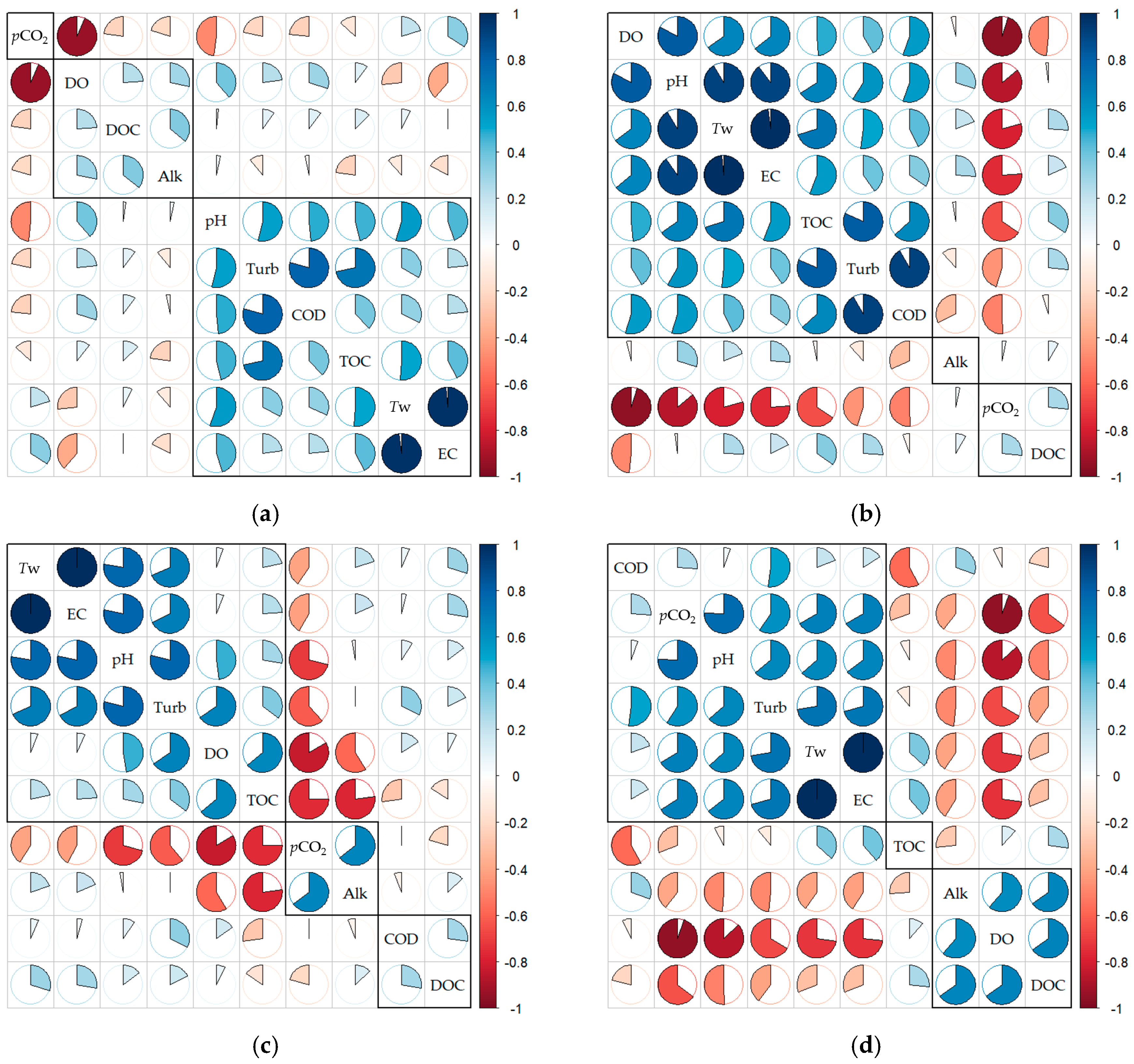
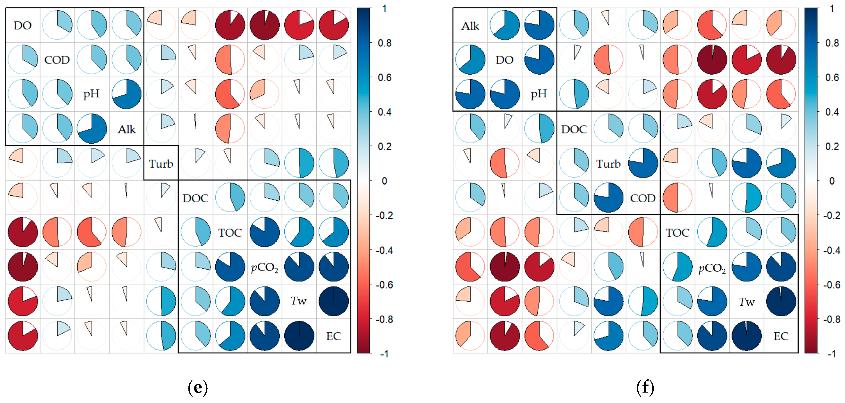
3.1. Summary Statistics and Correlation Analyses

The basic statistical values (minimum, maximum, medium, mean, and standard deviation) of the major environmental variables measured during the study period are shown in Table 1. The environmental variables covered the following ranges: pCO2 (215–6000 µatm), Tw (7.2–30.5 °C), Cond (130–187 μS·cm−1), DO (1.6–13.1 mg·L−1), pH (6.9–8.7), Turb (0.4–2.9 NTU), COD (1.2–10.3 mg·L−1), TOC (1.6–11.9 mg·L−1), DOC (1.6–8.3 mg·L−1), Chl-a (0.1–19.9 mg·m−3), and Alk (30.0–51.4 mg·L−1 as CaCO3).
Spearman correlation analysis was conducted to investigate correlations between measured variables, and the results are shown in Figure 2. Hierarchical cluster analysis was carried out, and grouping was performed using the complete-linkage clustering technique. According to an analysis of the entire dataset (Figure 2a), measured pCO2 was negatively correlated with all variables except Tw and Cond. In particular, the correlation coefficient with DO was −0.94, indicating a strong negative correlation.
The results observed at specific water depth (Figure 2b–f) also showed a strong negative correlation between measured pCO2 and DO; similar results were found between DO and pCO2 (R2 = 0.74, p < 0.001) in Janauca Lake in the Amazon River flood plain [44]. However, in that case, the DO concentration in water increased and the concentration of dissolved CO2 decreased due to active algal photosynthesis, which differs from the pattern observed in this study. The concentration of Chl-a (median = 1.1 mg·m−3) was very low in every layer except the surface layer in August and September, and the DO concentration in the reservoir mid-layer was decreased. Typically, DO concentration is influenced by gas exchange with the atmosphere, consumption by organic matter aerobic decomposition, and algal photosynthesis and respiration. Considering that measurements were taken primarily during the daytime during the survey period, DO reduction may have resulted largely from the decomposition of organic matter. Therefore, the strong inverse correlation between pCO2 and DO and increase in pCO2 in the water body may have been due to the aerobic decomposition of organic matter arising predominantly from the watershed.
The results from this study are consistent with those from previous studies [45,46,47,48], which demonstrate that DOC (allochthonous DOC) is an important source of CO2 supersaturation in terrestrial freshwater. Jonsson et al. [49] reported that pCO2 was increased due to aerobic decomposition of allochthonous DOC from the watersheds of 16 lakes in northern Sweden. However, the positive correlation shown between pCO2 and DOC in Jonsson et al. [49] was only observed herein at a water depth of 15 m (Figure 2e). This discrepancy may have arisen because most of the watershed DOC, which was transported via floodwaters, was decomposed before reaching the R4 site in front of the dam. The positive correlation between pCO2 and TOC, which is only evident in the mid-layer of the reservoir (15 and 20 m) where floodwaters containing organic matter were introduced, supports this inference.

3.2. Variations in Stratification Structure and Thermal Stability

Temporal changes in atmospheric temperature and the LN and St values analyzed by the rLakeAnalyzer are shown with temporal–depth changes in water temperature, as measured by the thermometer chain, in Figure 3a–d. Figure 3d also shows the dynamic changes in the metalimnion thickness and thermocline depth. The St and LN values were estimated using water temperature-with-depth data, which were measured at 10 min intervals from July 11 to December 31, 2017. During the study period, the atmospheric temperature ranged from a minimum of –9.1 °C to a maximum of 31 °C. LN ranged from 0.1 to 123.9, and St ranged from 9.6 to 2823.8 J·m−2.
At the beginning of the experiment on July 11, the air temperature was 26.7 °C and the St was 2383 J·m−2, displaying stable thermal stratification. The maximum stratification strength occurred on August 12, with a St of 2674 J·m−2. Then, a large amount of water entered the reservoir after five consecutive days of rainfall (125.5 mm), resulting in a temporary decrease in stratification strength. At this time, the LN value decreased sharply from 105.2 to 16.8, then increased to 120.6. The floodwaters propagated into the reservoir along the upper layer of the thermocline (the equal density layer) formed before the rainfall, increasing the depth of the existing thermocline from 15 m to 25 m and inducing an abrupt change in the thickness of the metalimnion layer.
As the air temperature dropped below 10 °C from October 30 onwards, the thickness of the metalimnion layer decreased sharply from 8.8 to 4.4 m, and the St weakened to 790.2 J·m−2. On November 27, the St had decreased to ~300 J·m−2, and the water layer was completely mixed up to a depth of 30 m, thereby removing most of the thermal stratification. As the atmospheric temperature decreased, the stratification became weaker, and the thermocline depth also tended to deepen gradually. In addition, the correlation between atmospheric temperature and stratification strength (St) was high, with a coefficient of 0.95.

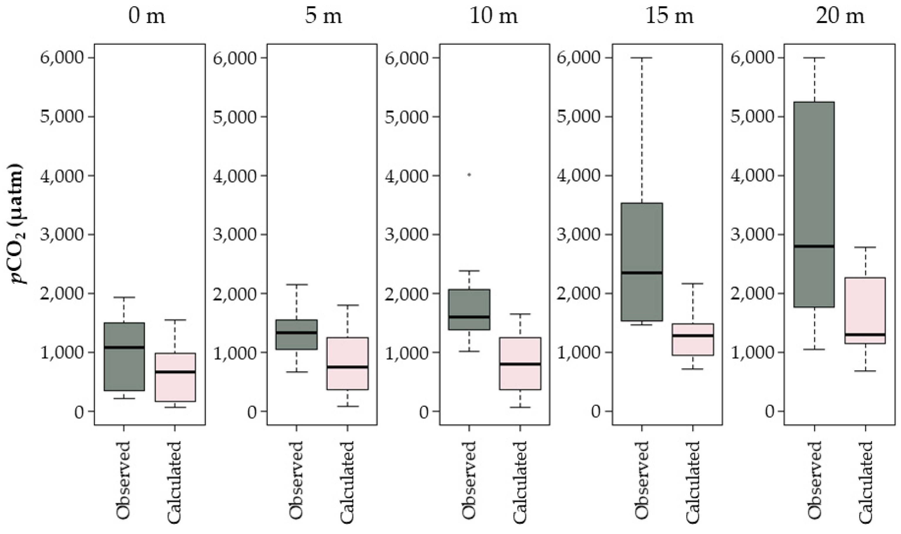
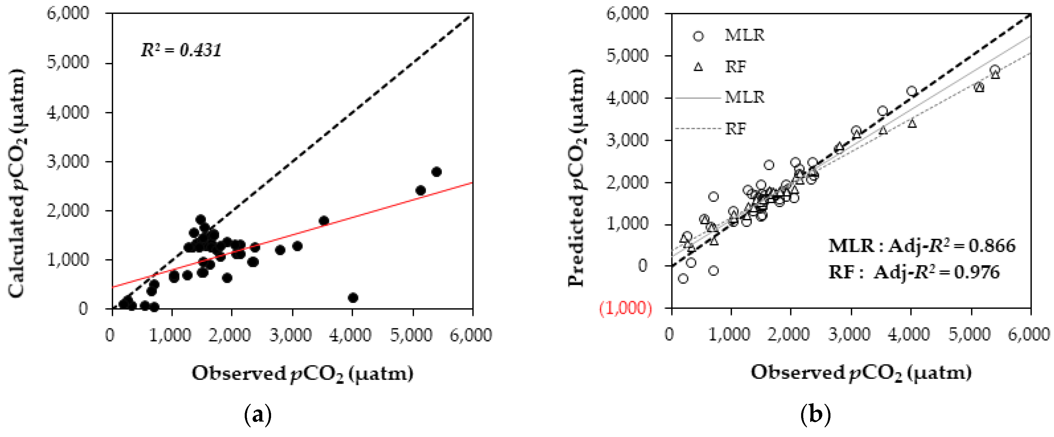
3.3. Comparisons of Measured and Estimated pCO2 Values

A total of 58 pCO2 values (µatm) measured with water depth were compared with the pCO2 values estimated by CO2SYS (Figure 4). The pCO2 values estimated by CO2SYS were 49.4% lower than the average measured pCO2. The RMSE between the estimated and measured pCO2 values was 1531 µatm for the entire dataset, 541 µatm for the surface layer (water depth = 0 m), and 2038 µatm for the bottom layer (water depth = 20 m). Thus, the deviation increased as the water depth increased (Figure 4). Moreover, the coefficient of determination (R2) was 0.43, indicating low significance. These results are consistent with previous studies performed at similar pH and DIC concentration ranges [32,35]. As mentioned in previous studies, this error between the measured and calculated pCO2 values can be attributed primarily to inaccurate pH measurements, and the error is greater at lower pH [35]. Furthermore, the dynamic variation in dissolved CO2 concentration—due to the decomposition of organic matter contained in floodwater introduced into the mid-layer of the reservoir—differs from the thermodynamic equilibrium assumption used by CO2SYS [6,47].
Thus, MLR and RF models were developed from major environmental variables to better predict pCO2 in water. The MLR model used a stepwise method for all explanatory variables, which included air pressure (Pa), Tw, Cond, DO, pH, COD, TOC, DOC, and Alk. Similar methods to those used in this study have been applied previously [35], however the previous study developed MLR and RF models using water quality data from only the surface layer of the water bodies (n = 10), and hence Chl-a and Turb—which herein showed little variation except in the surface layer—were determined to be major factors. In the current statistical evaluations, Chl-a and Turb contributed little to the prediction performance of the model; thus, they were excluded from the explanatory variables. The selected optimal MLR model included explanatory variables Tw, DO, pH, and DOC (Equation (1)). The Adj-R2 and AIC values were 0.866 and 577.5, respectively.
  p CO 2 = 95.24   ×   T w 440.87 × DO 1060.3   × pH 225.0 × DOC + 11 , 435.74  
The significance of the explanatory variables in the RF prediction model can be placed in the following order: DO > pH > Tw > Pa > Cond > Alk > DOC > COD > TOC. To prevent overfitting, cross validation was used to select the most parsimonious model; DO, pH, Tw, Pa, Cond, and DOC were selected as predictors, and Adj-R2 was 0.976, which indicates very high prediction performance (Figure 5).
The pCO2 measured by the NDIR method ranged from 215 to 6000 (mean = 2008) µatm, and the predicted values from the MLR and RF models ranged from −290 to 4679 (mean: 1797) µatm and 425 to 5525 (mean: 1895) µatm, respectively. The errors between the values estimated by the MLR and RF models and the measured values were 18.5% and 13.0%, respectively, which were much improved over the error for CO2SYS estimated values (49.4%) based on thermodynamic equilibrium theory (Figure 5). Thus, the unmeasured pCO2 values were estimated using the RF model, which featured the lowest error and superior prediction performance.

3.4. Dynamic Vertical Variations of pCO2 and Water Quality Variables

Temporal changes in daily precipitation (mm), daily mean wind speed (m·s−1), and Chl-a concentration in the surface layer (mg·m−3) are shown in Figure 6; the 12 campaign dates are denoted (a–l), respectively. Chl-a concentration data collected by K-water are also presented. Vertical profiles of pH, DOC, DO, and Tw for each survey date are shown in Figure 7. Variations of the pCO2 with depth are visualized along with the pCO2 predicted by the RF model and measured pCO2. The pCO2 measurement instrument failed after the July 27 measurement; the month of August was not included in the analysis.
On July 11 (Figure 7a), at the beginning of the study, thermal stratification was present. The pCO2 in the surface layer was 1542 µatm, and thus supersaturated rather than in equilibrium with the atmosphere. The pH was high nearer the surface, with values of 8.5 or more to a depth of 10 m, and relatively low (7.5) at 20 m. The vertical distribution of pCO2 was inversely correlated with pH, and the correlation coefficient was greater at a depth of 20 m than at the surface layer. DO sag phenomena occurred on July 20 (Figure 7b) and July 27 (Figure 7c); DO drastically decreased at depths of 5–15 m (the upper part of the thermocline was at 15 m). The pCO2 values were in the range of 3127–3155 µatm, and the DOC concentration was 2.448–2.738 mg·L−1, higher than the values at other water depths. The increase in pCO2 in the upper part of the thermocline was closely related to the rainfall event. Due to the 28.5 mm of rainfall experienced from July 14 to 15, a mid-layer density current containing organic matter flowed down to a depth of 10 m (i.e., in the upper part of the thermocline, which was equal in density current); this was related to the reduction in DO and pH and increase in pCO2 from organic matter decomposition. The maximum pCO2 values (3638–3895 µatm) were observed at depths of 10–12 m (above the thermocline) on July 27 (Figure 7c) after 25 mm of rainfall and again on July 24. Generally, heavy rainfall transports large amounts of organic matter from the watershed; pH decreases and pCO2 increases as organic matter decomposes in the water [50,51,52]. These results are consistent with a study by Jonsson et al. [47] showing high correlations between DOC concentration and pCO2 in 16 lakes in northern Sweden. In this study, aqueous pCO2 was supersaturated throughout the various DOC ranges (0.4–9.9 mg·L−1), which may have been caused by allochthonous DOC from the watershed and heterotrophic respiration in the reservoir.
On September 6 (Figure 7d), the thermocline was at a depth of 25 m, which was lower by about 10 m than that on July 27. The depths at which DO concentration was depleted and the pCO2 value was 2000 µatm or higher were extended to 10–30 m. The vertical distributions of pCO2, DO, and pH changed significantly as the floodwater, which included large amounts of organic matter, flowed into the upper part of the thermocline (25 m depth) after 57 mm of precipitation fell on July 31. The pCO2 of the surface layer was 346 µatm, which was undersaturated with regard to the atmospheric equilibrium state, but tended to significantly increase with increasing water depth. In particular, at a depth of 10 m, pCO2 had increased considerably to 4022 µatm and maintained similar concentrations up to 30 m in depth. DO was minimized at 10 m with a value of 1.59 mg/L, and the DO concentrations were low, with values of 3.87 mg/L or less down to 30 m. At this time, the maximum wind speed was 4.5 m·s−1, and the pCO2 in the surface layer seemed to be in equilibrium with the atmospheric concentration as a strong wind blew. In contrast, the drastic decrease in pCO2 in the surface layer in September was closely related to an increase in algal biomass after August (Chl-a concentration on August 2 = 1.0 mg·m−3 → September 7 = 7.8 mg·m−3) (Figure 6). Dense algae in the surface layer consume CO2 during the day and increase the DO [53]. This is consistent with previous studies suggesting that plankton metabolism significantly influences pCO2, and that higher DO concentrations are associated with lower CO2 emissions from the reservoir surface layer [20,44].
On September 12 (Figure 7e), the pCO2 in the surface layer was 410 µatm, similar to the atmospheric pCO2 level. Meanwhile, the pCO2 values at depths of 14–25 m were high, ranging from 4460 to 6000 µatm due to the decomposition of organic matter in floodwater. On October 10, the pCO2 in the surface layer was at its minimum value, of 215 µatm. However, the pCO2 in the mid-layer (depths of 14–25 m) maintained high values of 3000 µatm or more, possibly due to the heavy rainfall event (86.5 mm·day−1) on September 11. Drastic variations in DO, pH, and pCO2 were observed below the mixed-layer of the reservoir as large amounts of organic matter were introduced with the rainwater inflow and attendant organic matter decomposition.
As the thermal stratification strength weakened, the thermocline became deeper. On October 17 (Figure 7g), the pCO2 in the surface layer was 410 µatm, similar to the atmospheric concentration. However, the pCO2 was 2000 µatm or higher at depths of 10 m or less, gradually increasing with depth. On October 23 (Figure 7h), the pCO2 in the surface layer increased drastically to 1934 µatm, and similar pCO2 values (1751–2388 µatm) were observed from the surface layer to a depth of 25 m as the atmospheric temperature dropped and the thermocline weakened after October 10. At 30 m, the DO concentration was as low as 3.1 mg·L−1, and the pCO2 was 3640 µatm, the maximum value. These results indicate that the CO2 accumulated in the mid- and lower layers of the reservoir was transferred to the surface layer by vertical mixing as the thermal stratification in the reservoir weakened (St = 887 J·m−2, LN = 9.3). October 23 (Figure 7h) to November 21 (Figure 7l) featured similar vertical distributions of pCO2, pH, DO, and DOC from the surface layer to a depth of 28 m. However, at depths of 30 m and deeper, weak thermal stratification remained, the pH and DO concentration were lower, and the pCO2 was higher than in the completely mixed layer.

3.5. Temporal Variations of the CO2 NAF

The CO2 NAF between the reservoir surface and the atmosphere was estimated using the thin boundary layer method [54,55]. The difference between the measured pCO2 values in the water and the atmosphere was used as the concentration gradient. The gas exchange coefficient was derived as a function of wind speed and water temperature using the Wanninkhof and Knox [56] equation. The NAF shows (Figure 8) large temporal variations. There was an overall negative NAF (i.e., absorption of CO2 from the atmosphere) from July to mid-October, when the primary production of the reservoir increased with water temperature. This dramatically changed to a positive NAF (i.e., emission of CO2 from the reservoir) after the turnover event. On November 21, 2017, the NAF increased up to 3235 mg-CO2 m−2·day−1, and further to 16,519 mg-CO2 m-2·day−1 in January 2018 (not shown in Figure 8), which is much higher than the average NAF of 1400 mg-CO2 m−2·day−1 from other temperate reservoirs reported in Louis et al. [57]. These results suggest that the CO2 NAF in stratified reservoirs changes seasonally. Moreover, a large CO2 pulse emission could initiate at the reservoir surface during the turnover period.

4. Conclusions

Reservoirs have been reported as major emitters of GHGs, but the temporal variability of pCO2 in stratified reservoirs and CO2 pulse emissions mechanisms during fall turnover events have not been sufficiently studied. In this study, variations in pCO2 vertical distribution with stratification strength were examined in a monomictic reservoir located in a temperate region. pCO2 vertical mixing and supersaturation in the surface layer were explored, along with the changing thermal stratification structure before and after a turnover period in which thermal stratification was destroyed.
Calculations of pCO2 using pH and Alk values based on the thermodynamic equilibrium theory (in CO2SYS) showed increased error relative with increasing water depth; CO2SYS underestimated the measured values by 49.4%. This error can be attributed to inaccurate pH measurements and dynamic variation of the dissolved CO2 concentration due to the decomposition of organic matter, which differs from the thermodynamic equilibrium assumption used by CO2SYS. The MLR and RF models that were developed to estimate pCO2 in the reservoir showed greatly improved errors of 18.5% and 13.0%, respectively, compared to the mean measured pCO2 value.
The pCO2 distributions with water depth during the study period were closely related to rainfall events and the strength of the thermal stratification. Until the end of July, pCO2 was supersaturated in the surface layer and not in equilibrium with the atmosphere. However, after August, pCO2 rapidly decreased to below saturation as algae grew. In contrast, in the middle layer of the reservoir, floodwater carrying organic matter flowed into the upper part of the thermocline (the equal density layer after the rainfall event), and the middle layer DO concentration decreased due to the aerobic decomposition of the organic matter. Subsequent increases of the pCO2 were observed at the same layer. During periods of strong thermal stratification in the reservoir, high pCO2 values were maintained in the middle layer without spreading to the surface layer. However, after mid-October, when the stratification began to weaken, water instantly mixed between the upper and lower layers, producing relatively constant pCO2, pH, DO, and DOC from the surface to a depth of 28 m. As a result, the pCO2 in the surface layer increased sharply, and the pCO2 in the deep layer decreased, reaching equilibrium. These results suggest that large-scale CO2 pulse emissions were initiated at the reservoir surface during the turnover period.
The results of this study are important for understanding the carbon cycle in stratified reservoirs located in temperate zones, and particularly the “pulsed emissions” of carbon during turnover periods. However, as the study was conducted near the front of the dam, the results may not be representative of the whole domain of the Daecheong Reservoir. To analyze spatial variability, this study will be expanded to further locations in the Daecheong Reservoir in the future. In addition, the temporal and spatial changes of GHGs in the reservoir will be examined by applying numerical hydrodynamic and water quality modeling techniques, in order to comprehensively evaluate the processes of carbon emission from the stratified reservoir.

Author Contributions

Conceptualization, S.C. and H.P.; Field Experiments, H.P.; Models, H.P.; Formal Analysis, H.P.; Data Curation, S.C.; Writing, Original Draft Preparation, H.P.; Writing, Review and Editing, S.C.; Visualization, H.P.; Supervision, S.C.; Funding Acquisition, S.C.

Funding

This work was supported by a Korea Agency for Infrastructure Technology Advancement (KAIA) grant funded by the Ministry of Land, Infrastructure, and Transport (Grant number 18AWMP-B083066-05) and by the Basic Science Research Program of the National Research Foundation of Korea (NRF), which is funded by the Ministry of Education (Grant number 2016R1D1A3B03932308).

Conflicts of Interest

The authors declare no conflict of interest.

References

  1. IPCC. Climate change, the physical science basis. In Contribution of Working Group I to the Fifth Assessment Report of the Intergovernmental Panel on Climate Change; Cambridge University Press: Cambridge, NY, USA, 2013; ISBN 9781107057999. [Google Scholar]
  2. IPCC. Climate change, synthesis report. In Contribution of Working Groups I, II and III to the Fifth Assessment Report of the Intergovernmental Panel on Climate Change; IPCC: Geneva, Switzerland, 2014; ISBN 978-92-9169-143-2. [Google Scholar]
  3. IPCC National Greenhouse Gas Inventories Programme. IPCC Guidelines for National Greenhouse Gas Inventories; IGES: Hayama, Japan, 2006; ISBN 4-88788-032-4. [Google Scholar]
  4. Battin, T.J.; Luyssaert, S.; Kaplan, L.A.; Aufdenkampe, A.K.; Richter, A.; Tranvik, L.J. The boundless carbon cycle. Nat. Geosci. 2009, 2, 598–600. [Google Scholar] [CrossRef]
  5. Cole, J.J.; Prairie, Y.T.; Caraco, N.F.; McDowell, W.H.; Tranvik, L.J.; Striegl, R.G.; Duarte, C.M.; Kortelainen, P.; Downing, J.A.; Middelburg, J.J.; et al. Plumbing the Global Carbon Cycle: Integrating Inland Waters into the Terrestrial Carbon Budget. Ecosystems 2007, 10, 171–184. [Google Scholar] [CrossRef]
  6. Golub, M. Controls on Temporal Variation in Ecosystem-Atmosphere Carbon Dioxide Exchange in Lakes and Reservoirs. Ph.D. Thesis, University of Wisconsin-Madison, Madison, WI, USA, November 2016. [Google Scholar]
  7. Wetzel, R.G. Limnology: Lake and River Ecosystems; Academic Press: New York, NY, USA, 2001; ISBN 9780127447605. [Google Scholar]
  8. Cole, J.J.; Caraco, N.F.; Kling, G.W.; Kratz, T.K. Carbon dioxide supersaturation in the surface waters of lakes. Science 1994, 265, 1568–1570. [Google Scholar] [CrossRef] [PubMed]
  9. Algesten, G.S.; Sobek, A.K.; Bergstrom, A.; Agren, L.; Tranvik, J.; Jansson, M. Role of lakes for organic carbon cycling in the boreal zone. Glob. Chang. Biol. 2003, 10, 141–147. [Google Scholar] [CrossRef]
  10. Roehm, C.L.; Prairie, Y.T.; del Giorgio, P.A. The pCO2 dynamics in lakes in the boreal region of northern Québec, Canada. Glob. Biogeochem. Cycles 2009. [Google Scholar] [CrossRef]
  11. Einsele, G.; Yan, J.; Hinderer, M. Atmospheric carbon burial in modern lake basins and its significance for the global carbon budget. Glob. Planet. Chang. 2001, 30, 167–195. [Google Scholar] [CrossRef]
  12. Kortelainen, P.; Rantakari, M.; Huttunen, J.T.; Mattsson, T.; Alm, J.; Juutinen, S.; Larmola, T.; Silvola, J.; Martikainen, P.J. Sediment respiration and lake trophic state are important predictors of large CO2 evasion from small boreal lakes. Glob. Chang. Biol. 2006, 12, 1554–1567. [Google Scholar] [CrossRef]
  13. Stallard, F.R. Terrestrial sedimentation and the C cycle: Coupling weathering and erosion to carbon storage. Glob. Biogeochem. Cycles 1998, 12, 231–257. [Google Scholar] [CrossRef]
  14. Tranvik, L.J.; Downing, J.A.; Cotner, J.B.; Loiselle, S.A.; Striegl, R.G.; Ballatore, T.J.; Dillon, P.; Finlay, K.; Fortino, K.; Knoll, L.B.; et al. Lakes and reservoirs as regulators of carbon cycling and climate. Limnol. Oceanogr. 2009, 54, 2298–2314. [Google Scholar] [CrossRef] [Green Version]
  15. Downing, J.A.; Cole, J.J.; Middelburg, J.J.; Striegl, R.G.; Duarte, C.M.; Kortelainen, P.; Prairie, Y.T.; Laube, K.A. Sediment organic carbon burial in agriculturally eutrophic impoundments over the last century. Glob. Biogeochem. Cycles 2008. [Google Scholar] [CrossRef]
  16. Lehner, B.; Liermann, C.R.; Revenga, C.; Vörösmarty, C.; Fekete, B.; Crouzet, P.; Döll, P.; Endejan, M.; Freken, K.; Magome, J.; et al. High-resolution mapping of the world’s reservoirs and dams for sustainable river-flow management. Front. Ecol. Environ. 2011, 9, 494–502. [Google Scholar] [CrossRef]
  17. Winslow, L.A.; Read, J.S.; Hanson, P.C.; Stanley, E.H. Lake shoreline in the contiguous United States: Quantity, distribution and sensitivity to observation resolution. Freshw. Biol. 2013, 59, 213–223. [Google Scholar] [CrossRef]
  18. Prairie, Y.T.; Alm, J.; Beaulieu, J.; Barros, N.; Battin, T.; Cole, J.; del Giorgio, P.; DelSontro, T.; Guérin, F.; Harby, A.; et al. Greenhouse Gas Emissions from Freshwater Reservoirs: What Does the Atmosphere See? Ecosystems 2018, 21, 1058–1071. [Google Scholar] [CrossRef]
  19. Deemer, B.R.; Harrison, J.A.; Li, S.; Beaulieu, J.J.; DelSontro, T.; Barros, N.; Bezerra-neto, J.F.; Powers, S.M.; Santos, M.; Vonk, J.A. Greenhouse Gas Emissions from Reservoir Water Surfaces: A New Global Synthesis. BioScience 2016, 66, 949–964. [Google Scholar] [CrossRef] [Green Version]
  20. Bevelhimer, M.S.; Stewart, A.J.; Fortner, A.M.; Phillips, J.R.; Mosher, J.J. CO2 is Dominant Greenhouse Gas Emitted from Six Hydropower Reservoirs in Southeastern United States during Peak Summer Emissions. Water 2016, 8, 15. [Google Scholar] [CrossRef]
  21. Denfeld, B.A.; Wallin, M.B.; Sahlee, E.; Sobek, S.; Kokic, J.; Chmiel, H.E.; Weyhenmeyer, G.A. Temporal and spatial carbon dioxide concentration patterns in a small boreal lake in relation to ice-cover dynamics. Boreal Environ. Res. 2015, 20, 679–692. [Google Scholar]
  22. Laas, A.; Cremona, F.; Meinson, P.; Rõõm, E.; Nõges, T.; Nõges, P. Summer depth distribution profiles of dissolved CO2 and O2 in shallow temperate lakes reveal trophic state and lake type specific differences. Sci. Total Environ. 2016, 566, 63–75. [Google Scholar] [CrossRef] [PubMed]
  23. McDonald, C.P.; Stets, E.G.; Striegl, R.G.; Butman, D. Inorganic carbon loading as a primary driver of dissolved carbon dioxide concentrations in the lakes and reservoirs of the contiguous United States. Glob. Biogeochem. Cycles 2013, 27, 285–295. [Google Scholar] [CrossRef] [Green Version]
  24. Ballantyne, A.P.; Andres, R.; Houghton, R.; Stocker, B.D.; Wanninkhof, R.; Anderegg, W.; Cooper, L.A.; DeGrandpre, M.; Tans, P.P.; Miller, J.B.; et al. Audit of the global carbon budget: Estimate errors and their impact on uptake uncertainty. Biogeosciences 2015, 12, 2565–2584. [Google Scholar] [CrossRef]
  25. Wang, F.; Cao, M.; Wang, B.; Fu, J.; Luo, W.; Ma, J. Seasonal variation of CO2 diffusion flux from a large subtropical reservoir in East China. Atmos. Environ. 2015, 103, 129–137. [Google Scholar] [CrossRef]
  26. Mosher, J.J.; Fortner, A.M.; Phillips, J.M.; Bevelhimer, M.S.; Stewart, A.J.; Troia, M.J. Spatial and temporal correlates of greenhouse gas diffusion from a hydropower reservoir in the Southern United States. Water 2015, 7, 5910–5927. [Google Scholar] [CrossRef]
  27. Yang, M.; Grace, J.; Geng, X.; Guan, L.; Zhang, Y.; Lei, J.; Lu, C.; Lei, G. Carbon Dioxide Emissions from the Littoral Zone of a Chinese Reservoir. Water 2017, 9, 539. [Google Scholar] [CrossRef]
  28. Bastien, J.; Demarty, M.; Tremblay, A. CO2 and CH4 diffusive and degassing fluxes from 2003 to 2009 at Eastmain 1 reservoir, Québec, Canada. Inland Waters 2011, 1, 113–123. [Google Scholar] [CrossRef]
  29. Demarty, M.; Bastien, J.; Tremblay, A. Annual follow-up of gross diffusive carbon dioxide and methane emissions from a boreal reservoir and two nearby lakes in Québec, Canada. Biogeosciences 2011, 8, 41–53. [Google Scholar] [CrossRef] [Green Version]
  30. Beaulieu, J.J.; Smolenski, R.L.; Nietch, C.T.; Townsend-Small, A.; Elovitz, M.S. High methane emissions from a midlatitude reservoir draining an agricultural watershed. Environ. Sci. Technol. 2014, 48, 11100–11108. [Google Scholar] [CrossRef] [PubMed]
  31. K-Water. Available online: http://english.kwater.or.kr/ (accessed on 31 July 2018).
  32. UNESCO/IHA. GHG Measurement Guidelines for Freshwater Reservoirs; International Hydropower Association: London, UK, 2010; ISBN 978-0-9566228-0-8. [Google Scholar]
  33. APHA. Standard Methods for the Examination of Water and Wastewater, 21st ed.; American Public Health Association/American Water Works Association/Water Environment Federation: Washington, DC, USA, 2005; ISBN 9780875530475. [Google Scholar]
  34. Lewis, E.; Wallace, D. Program Developed for CO2 System Calculations; Department of Applied Science Brookhaven National Laboratory: Upton, NY, USA, 1998. [Google Scholar] [CrossRef]
  35. Raymond, P.A.; Caraco, N.F.; Cole, J.J. Carbon dioxide concentration and atmospheric flux in the Hudson River. Estuaries Coasts 1997, 20, 381–390. [Google Scholar] [CrossRef]
  36. Wang, Z.A.; Bienvenu, D.J.; Mann, P.J.; Hoering, K.A.; Poulsen, J.R.; Spencer, R.G.M. Holmes, R.M. Inorganic carbon speciation and fluxes in the Congo River. Geophys. Res. Lett. 2013, 40, 511–516. [Google Scholar] [CrossRef]
  37. Chung, S.W.; Park, H.S.; Yoo, J.S. Variability of pCO2 in surface waters and development of prediction model. Sci. Total Environ. 2018, 622–623, 1109–1117. [Google Scholar] [CrossRef] [PubMed]
  38. Breiman, L. Random forests. Mach. Learn. 2001, 45, 5–32. [Google Scholar] [CrossRef]
  39. Hebbali, A. Tools for Teaching and Learning OLS Regression. 2017. Available online: https://rsquaredacademy.github.io/olsrr/ (accessed on 31 July 2018).
  40. Liaw, A.; Wiener, M. Classification and regression by random forest. R News. 2002, 2, 18–22. Available online: https://www.r-project.org/doc/Rnews/Rnews_2002-3.pdf (accessed on 31 December 2002).
  41. Winslow, L.A.; Read, J.S.; Woolway, R.; Brentrup, J.; Leach, T.; Zwart, J.; Albers, S.; Collinge, D. Lake Physics Tools. 2017. Available online: https://github.com/GLEON/rLakeAnalyzer (accessed on 31 July 2018).
  42. Idso, S.B. On the concept of lake stability. Limnol. Oceanogr. 1973, 18, 681–683. [Google Scholar] [CrossRef] [Green Version]
  43. Imberger, J.; Patterson, J.C. Physical limnology. Adv. App. Mech. 1989, 27, 303–475. [Google Scholar] [CrossRef]
  44. Amaral, J.H.; Borges, A.V.; Melack, J.M.; Sarmento, H.; Barbosa, P.M.; Kasper, D.; Melo, M.L.; Fex-Wolf, D.D.; Silva, J.S.; Forsberg, B.R. Influence of plankton metabolism and mixing depth on CO2 dynamics in an Amazon floodplain lake. Sci. Total Environ. 2018, 630, 1381–1393. [Google Scholar] [CrossRef] [PubMed]
  45. dos Santos, M.A.; Rosa, L.P.; Sikar, B.; Sikar, E.; dos Santos, E.O. Gross greenhouse gas fluxes from hydro-power reservoir compared to thermos-power plants. Energy Policy 2006, 34, 481–488. [Google Scholar] [CrossRef]
  46. Tadonléké, R.D.; Marty, J.; Planas, D. Assessing factors underlying variation of CO2 emissions in boreal lakes vs. reservoirs. FEMS Microbiol. Ecol. 2012, 79, 282–297. [Google Scholar] [CrossRef] [PubMed]
  47. Pacheco, F.S.; Roland, F.; Downing, J.A. Eutrophication reverses whole-lake carbon budgets. Inland Waters 2013, 4, 41–48. [Google Scholar] [CrossRef]
  48. Hanson, P.C.; Pace, M.L.; Carpenter, S.R.; Cole, J.J.; Stanley, E.H. Integrating landscape carbon cycling: Research needs for resolving organic carbon budgets of lakes. Ecosystems 2015, 18, 363–375. [Google Scholar] [CrossRef]
  49. Jonsson, A.; Karlsson, J.; Jansson, M. Sources of carbon dioxide supersaturation in clearwater and humic lakes in northern Sweden. Ecosystems 2003, 6, 224–235. [Google Scholar] [CrossRef]
  50. Jones, S.E.; Kratz, T.K.; Chiu, C.Y.; McMahon, K.D. Influence of typhoons on annual CO2 flux from a subtropical, humic lake. Glob. Chang. Biol. 2009, 15, 243–254. [Google Scholar] [CrossRef]
  51. Marotta, H.; Duarte, C.M.; Pinho, L.; Enrich-Prast, A. Rainfall leads to increased pCO2 in Brazilian coastal lakes. Biogeosciences 2010, 7, 1607–1614. [Google Scholar] [CrossRef] [Green Version]
  52. Pquay, F.S.; Mackenzie, F.T.; Borges, A.V. Carbon dioxide dynamics in rivers and coastal waters of the “big island” of Hawaii, USA, during baseline and heavy rain conditions. Aquat. Geochem. 2007, 13, 1–18. [Google Scholar] [CrossRef]
  53. McManus, J.; Heinen, E.A.; Baehr, M.M. Hypolimnetic oxidation rates in Lake Superior: Role of dissolved organic material on the lake’s carbon budget. Limnol. Oceanogr. 2003, 48, 1624–1632. [Google Scholar] [CrossRef]
  54. Liss, P.; Slater, P. Fluxes of gases across the air-sea interface. Nature 1974, 247, 181–184. [Google Scholar] [CrossRef]
  55. Cole, J.; Prairie, Y.T. Dissolved CO2. In Encyclopedia of Inland Waters; Elsevier Science & Technology: Amsterdam, The Netherlands, 2009; pp. 30–34. [Google Scholar] [CrossRef]
  56. Wanninkhof, R.; Knox, M. Chemical enhancement of CO2 exchange in natural waters. Limnol. Oceanogr. 1996, 41, 689–697. [Google Scholar] [CrossRef]
  57. Louis, V.L.; Kelly, C.A.; Duchemin, É.; Rudd, J.W.M.; Rosenberg, D.M. Reservoir Surfaces as Sources of Greenhouse Gases to the Atmosphere: A Global Estimate: Reservoirs are sources of greenhouse gases to the atmosphere, and their surface areas have increased to the point where they should be included in global inventories of anthropogenic emissions of greenhouse gases. BioScience 2000, 50, 766–775. [Google Scholar] [CrossRef]
Figure 1. Location of the study site and monitoring station.
Water 10 01347 g001
Figure 2. Spearman correlation coefficients between environmental variables and pCO2 at (a) all depths (n = 45), (b) 0 m (n = 9), (c) 5 m (n = 9), (d) 10 m (n = 9), (e) 15 m (n = 9), and (f) 20 m (n = 9).
Water 10 01347 g002aWater 10 01347 g002b
Figure 3. Temporal variations of (a) air temperature, (b) Lake number (LN), (c) Schmidt stability (St), and (d) time–depth profile of water temperature.
Water 10 01347 g003
Figure 4. Box plot comparisons of observed (nondispersive infrared method) and calculated (pH/Alk method using CO2SYS) pCO2 by depth (0, 5, 10, 15, and 20 m).
Water 10 01347 g004
Figure 5. Observed pCO2 (NDIR method) compared to (a) calculated pCO2 (CO2SYS estimations) and (b) predicted pCO2 (MLR and RF models).
Water 10 01347 g005
Figure 6. Temporal variations in daily precipitation, wind speed, and chlorophyll a concentration (Chl-a) during the monitoring period: the arrows indicate 12 campaign dates.
Water 10 01347 g006
Figure 7. Dynamic vertical distributions of water temperature (Tw), pH, dissolved organic carbon (DOC), dissolved oxygen (DO), and pCO2. The observed pCO2 values were measured in situ using the NDIR method.
Water 10 01347 g007
Figure 8. Temporal variations of CO2 net atmospheric flux (NAF) during the monitoring period. Negative and positive values indicate absorption and emission of CO2, respectively.
Water 10 01347 g008
Table 1. Descriptive statistics of the observed variables.
IndexpCO21
(µatm)
Tw 2
(°C)
Cond 3
(μS·cm−1)
DO 4
(mg·L−1)
pHTurb 5
(NTU)
COD 6
(mg·L−1)
TOC 7
(mg·L−1)
DOC 8
(mg·L−1)
Chl-a 9
(mg·m−3)
Alk 10
(mg·L−1 as CaCO3)
nobs115820020020020016020020020094200
Min2157.21301.66.90.40.21.61.60.130.0
Max600030.518713.18.72.910.311.98.319.951.4
median153821.41577.17.40.82.52.52.61.142.0
Mean208521.3154.46.77.51.02.62.72.73.142.2
std dev15294.714.12.20.40.61.31.50.74.93.1
1 Partial pressure of CO2; 2 Water temperature; 3 Electric conductivity; 4 Dissolved oxygen; 5 Turbidity; 6 Chemical oxygen demand; 7 Total organic carbon; 8 Dissolved organic carbon; 9 Chlorophyll a; 10 Alkalinity; 11 number of observations.

