Experimental and Simulation Investigation on the Kinetic Energy Dissipation Rate of a Fixed Spray-Plate Sprinkler


1
School of Water Conservancy and Environment, Zhengzhou University, Zhengzhou 450001, China
2
College of Water Resources and Architectural Engineering, Northwest A&F University, Yangling 712100, Shaanxi, China
*
Author to whom correspondence should be addressed.
Water 2018, 10(10), 1365; https://doi.org/10.3390/w10101365
Submission received: 2 September 2018
/
Revised: 23 September 2018
/
Accepted: 28 September 2018
/
Published: 30 September 2018
(This article belongs to the Special Issue Precision Agriculture and Irrigation)
Abstract
:Sprinkler irrigation is promoted due to its remarkable advantages in water conservation, but the high energy consumption limits its development in a situation of energy scarcity. In order to determine the energy consumption of a fixed spray-plate sprinkler (FSPS), its discharge and initial trajectory velocity were investigated using a particle image velocimetry (PIV) technique and computational fluid dynamics (CFD) analyses. A nozzle diameter of 4.76 mm was used under windless conditions. Overall, good agreement between simulation results and experimental values was obtained. On the premise that the simulation method produced high accuracy, a series of simulations was performed with different nozzle diameters. The water distribution pattern, stream trajectory velocity and kinetic energy dissipation were analyzed. The results show that the jet produced at the nozzle is split by grooves after it hits the plate, with separation occurring earlier with decreasing nozzle diameter. The area of the flow cross-section of the outlet is mainly influenced by nozzle diameter rather than working pressure. The initial trajectory velocity of the grooves increases logarithmically with increasing working pressure. A high working pressure may not cause large kinetic energy dissipation. The dissipation rate of the FSPS ranged from 28.01–50.97%, i.e., a large kinetic energy rate was observed. To reduce this energy dissipation and improve water use efficiency, the structure of the FSPS should be optimized in further research.
1. Introduction
Agricultural production consumes enormous amounts of water, which is a threat to water resources [1]. Sprinkler irrigation is characterized by high levels of water conservation [2,3,4,5]. Commonly, linear-move and center-pivot irrigation machines are widely used for their high degree of automation [6]. The earlier sprinklers equipped in these machines were high-pressure impact, and in recent years, increasing energy costs have shifted the focus to increasing the energy efficiency of agricultural sprinkler applications and led to the development of various low-pressure sprinklers. The two main low-pressure spray-plate sprinklers are the rotating spray-plate sprinkler (RSPS) and fixed spray-plate sprinkler (FSPS) [7]. Compared with RSPS, the fixed spray-plate sprinkler (FSPS) offers the advantages of a relatively low working pressure, high wind resistance and low cost [2,8,9,10]. The working principle of the FSPS is simple: a jet of water from a nozzle strikes a refraction cone and forms a series of nappe adherences in the spray-plate grooves. The water distribution pattern from a single FSPS resembles a wetted circular crown [11]. However, as the water strikes the refraction cone, the energy lost at the plate is extremely large, creating uncertainty about the initial velocity of the drops [12]. The initial trajectory velocity across the grooves is less than the jet velocity from the nozzle. This results in a reduction in the wetted width and control area during the irrigation with a liner-move irrigation machine [13]. In order to evaluate energy utilization efficiency, research on kinetic energy dissipation is required.
The kinetic energy is mainly influenced by the velocity and discharge of the liquid. In general, the outlet flux of each groove and nozzle can be obtained using a weighing method. The calculation of initial jet velocity from the nozzle requires a measurement of flux, which is then divided by the nozzle area. However, the FSPSs used in pivot and linear movement irrigation systems are different from impact sprinklers [6], i.e., the jet produced at the nozzle undergoes an inelastic shock after it hits the plate, causing a large reduction in trajectory velocity [12]. Therefore, the main problem in calculating kinetic energy dissipation is in obtaining the initial trajectory velocity.
Considering the handicap in estimating the initial trajectory velocity of FSPS, an experimental measurement was performed by Sánchez-Burillo et al. [12] using the photographic method. The instantaneous drop velocity vector at a bounded region close to the sprinkler was measured. Furthermore, a large head loss at the spray-plate was attained. By using the technique of low speed photography, Ouazaa et al. [14] determined drop velocity at a measurement point just after the plate, and the results showed that kinetic energy losses decreased with nozzle diameter increments. It is important to note that photographic method is available to acquire the initial trajectory velocity of FSPS. Besides, as one of photographic methods, the technique of particle image velocimetry (PIV) [15,16,17] can also be used in the measurement of jet velocity. The fundamental PIV is simple: once the fluid motion is received by the CCD camera, the positions of the droplet can be recorded at two instances of time, i.e., the droplet displacement, so it is realizable to calculate the trajectory velocity [18,19].
However, the measurement of velocity using the photographic method is inconvenient due to the requirement of a suitable experimental apparatus; in addition, the analysis of a large amount of samples is time consuming. With the development of computer technology and computational fluid dynamics (CFD) in recent years, numerical simulation has been widely used, as it offers the advantage of high efficiency [20,21]. Research on the initial trajectory velocity of a water jet has mainly focused on the free surface between the air and water. The interface tracking method, volume of fluid (VOF), which was proposed by Hirt and Nichols [22], providing insight into the underlying processes critical for primary and secondary atomization, is suitable in this regard [23,24,25]. In recent years, a coupled VOF with the level set method (LS-VOF) proposed by Osher and Sethian [26] has been tested by comparison against a standard VOF solver and experimental observation [27], and the result indicated that the LS-VOF model can improve surface tension implementation and provide a smooth variation of the physical properties across the interface between two fluids. Moreover, Jiang et al. [17] and Meredith et al. [28] have shown that the multiphase LS-VOF model can be successfully applied to simulate the performance of sprinklers.
Several articles have been published describing the kinetic energy losses of FSPS [12,14,29]; unfortunately, these data were collected using the experimental method. Considering that a limited number of studies have been carried out on the simulation of the initial trajectory velocity and kinetic energy dissipation rate of a FSPS, the objectives of this study are as follows: (1) use a PIV technique to determine the stream jet velocity from the grooves at different working pressures with a nozzle diameter of 4.76 mm; (2) investigate the flux and jet velocity of each groove using the numerical simulation method, and estimate the validity of numerical simulation results; (3) based on these simulation results of different nozzle diameters, analyze the water distribution pattern, jet velocity of the stream and kinetic energy dissipation of FSPS.
2. Experimental Setup
The selected FSPS was a Nelson D3000 (Nelson Irrigation Co., Walla Walla, WA 99362-2271, USA). The FSPS was equipped with a 4.76 mm diameter nozzle and a deflector plate with 36 grooves (Figure 1). The diameter of the spray-plate was 31 mm and had a cone with a height of 2.8 mm at its center. The nozzle was installed 12.5 mm above the spray-plate. During operation, the water jet from the nozzle hits the deflector, dividing the flow into 36 streams.
An experimental test (Figure 2) to evaluate the velocity of the stream was set up at the Irrigation Hydraulics Experiment Station at Northwest Agriculture and Forestry University, Yangling, China. It consisted of a water jet system and PIV system. The water jet system was comprised of: (1) a booster pump of 2.2 kW, which was controlled by a frequency conversion cabinet; (2) a water tank with a capacity of 0.5 m3; (3) a Nelson D3000 sprinkler coupled with a deflector plate with 36 grooves; and (4) a 32 mm diameter flow pipe and pressure sensor. The PIV system used to obtain the jet velocity consisted of: (1) a digital high-speed video camera (hotshot 512 sc); (2) a computer to collect data; and (3) analysis display software (MOVIAS Pro) for image processing. The experiment was performed using PIV visualization technology, i.e., PIV technology based on high-speed photography. As such, when the water stream jetted from the groove, the CCD camera recorded the scattered light distribution of the droplets at short intervals. The travel length over a fixed time was then processed using the MOVIAS Pro software and the velocity of the water jet calculated.
In general, the operating pressure could be adjusted between 34 and 413 kPa; accordingly, the working pressures were set to 50, 100, 150, 200 and 250 kPa. As the deflector plate had a tri-sectional structure and the grooves in each tri-section zone were symmetrical, the number of experimental grooves could be reduced to six. All experimental measurements were performed under windless conditions. As each stream jetting from a groove was relatively independent [30], each coherent jet emitted by the groove could be measured. In order to achieve high resolution images, the area of interest was set to 1280 × 800 pixels and the frames per second to 1000. Each measurement lasted for 2 min, and more than 20 drops for every combination were analyzed.
3. Numerical Simulation
3.1. Description of the Model
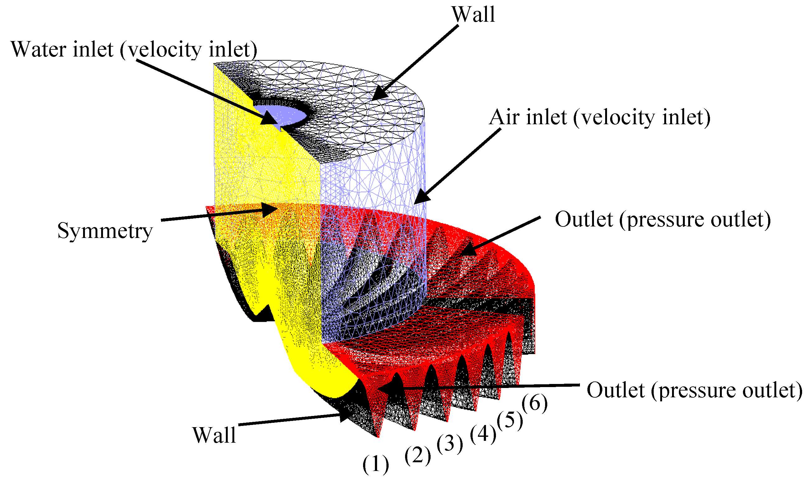
According to the actual size of the sprinkler, a three-dimensional flow region model was developed using the software Pro/Engineer. Considering the geometric symmetry of the FSPS, a symmetrical boundary condition was applied along a symmetry plane, i.e., only half of the domain was modeled. An unstructured mesh was used for the simulation domain using ANSYS ICEM software. Based on the experimental model, the boundaries of the numerical model were set as (i) the walls, (ii) the water inlet, (iii) the outlet, (iv) the air inlet and (v) symmetry (Figure 3). The Number 1 groove is located in the beginning of the tri-section; the Number 6 groove is near the symmetry axis of the trisection. A no-slip condition was applied to the walls; a velocity inlet condition was applied to the water and air inlets, and a pressure outlet condition was applied to the outlet. For mesh roughness to have a significant influence on the sharpness of the interface between air and water, a grid refinement of the groove outlet was performed. The calculation of initial jet velocity requires discharge to be measured, which is then divided by the nozzle area. The initial velocities for the water inlet at different working pressures are presented in Table 1.
3.2. Governing Equations
The numerical simulations were carried out using the CFD software ANSYS FLUENT 17.0. The mass conservation equation and Navier–Stokes equations for incompressible, viscous flow are given by Equations (1) and (2) [31,32]:
where ρ is fluid density (kg/m3); t is time; u is the flow velocity vector (m/s); p is pressure; u, v, w are averaged flow velocity components in the Cartesian coordinates x, y, and z, respectively (m/s); Fx, Fy, Fz are body forces, Fx = 0, Fy = 0, Fz = −ρg(N); and μ is dynamic viscosity (N s/m2). The concepts of div (divergence) and grad (gradient) are introduced as: .
In order to close the Navier–Stokes equations, the standard k-ε turbulence model was chosen to solve the unsteady calculation. The standard k-ε three-dimensional turbulence model is obtained from the following transport equations:
where k is turbulence kinetic energy (m2/s2); ε is turbulence dissipation (kg·m2/s3); i and j are vectors; and Cε1, Cε1 and σε are correcting coefficients.
The multiphase LS-VOF model was adopted for this study, offering the advantages of fewer iterative steps and lower computation time. Standard wall functions were applied as the near-wall treatment. The SIMPLE algorithm (semi-implicit method for the pressure-linked equations) was chosen to solve mass conservation and the Navier–Stokes equations. A second-order upwind scheme for the discretization of momentum, turbulent kinetic energy and turbulent dissipation rate was selected. The gravity and operating air pressure were set to 9.81 m/s2 and 101,325 Pa, respectively. The time step size (t) was set to 0.001 s, and the convergence precision was set to 0.0001 for all equations.
4. Results
Experimental data for flow rates and jet velocities were collected to compare with the simulation results. In general, the average velocities of water jetting from the grooves could not be obtained directly through the simulations; however, they could be calculated since the parameters of flow cross-section and mass flow rate were obtained. In order to obtain the cross-sectional area, the outlet flow pattern of each groove was observed through simulation with a 4.76 mm nozzle at the working pressure of 200 kPa, and Auto-CAD software was used to analyze the cross-sectional area. Cooperating with the simulation results of flux, the velocity with different volume fractions of water could be calculated. Figure 4 illustrates the calculated velocity of each groove with different water volume fractions. The velocity showed a large range of variation as the volume fraction changed from 0.3–0.8. The measured velocities, which ranged from 14.51 m/s–16.02 m/s, were used to calibrate the flow cross-section. In Figure 4, almost all the calculate velocities with a volume fraction of 0.5 and 0.6 were embraced in that region. Consequently, the shape of the free surface was determined from the water volume fraction using the ratio 0.55:1.
4.1. Comparison of Experimental Results and Simulated Values
Figure 5 illustrates the discharge of the 1st–6th groove, showing numerical simulation values (SVs) and experimental values (EVs). As shown, for the EVs at different working pressures, the flow rates increased when the groove number was increased from 1–6. The SVs showed a tendency to decrease slightly at the second groove and then increase, i.e., the minimum flow rate appeared at the second groove. Figure 5 also shows the phenomenon that all the SVs for the first groove were larger than the EVs, with relative errors of 2.60, 2.30, 3.15, 3.91 and 3.40%, respectively, for working pressures from 50–250 kPa. Conversely, the SVs were smaller than the EVs in the second groove, with a maximum relative error smaller than 1.94%. The primary reason for this was that a symmetry boundary condition was applied, meaning that scalar flux across this boundary was zero, and circumferential water movement to the boundary was ignored. The maximum relative error was no larger than 3.91% for all working conditions, implying that the SVs were close to the experimental results. In addition, when the working pressure was fixed, the maximum and minimum EVs for the six grooves showed a large difference (the same was true for the SVs). For example, when the working pressure was 50 kPa, the maximum and minimum flow rate EVs were 0.0165 m3/h and 0.0202 m3/h, respectively, i.e., a 20% difference (under the same conditions, the difference in the SVs was about 19.22%).
Velocity is an important parameter for evaluating the difference between the simulated and experimental results. The reported velocity of each stream was the average velocity calculated from flow rate divided by flow cross-section, as mentioned above. The free surface of the water outlet profile was determined in the calibration process. Numerical jet velocity results for the different working pressures were compared with the experimental results. Table 2 presents the data for six grooves at five working pressures. It shows that the relative deviation (RD) of each working pressure was smaller than 10%. When the working pressure was increased from 50–250 kPa, the maximum RD was 3.28, −4.07, 3.71%, 5.81 and 9.44% respectively, i.e., a generally increasing trend. The reason for this is that a higher working pressure yields a higher jet velocity as a large measurement error exists when the experimental jet velocity is high, and the simulation process neglected this factor. However, a good agreement between the simulation results and experimental values was obtained, which indicates that both PIV measurement and CFD simulation with the LS-VOF method could be used to analyze the jet velocity and discharge of the stream.
4.2. Fluid-Phase Nephogram and Initial Trajectory Velocity
Given the satisfactory agreement between the experimental and simulation results, the simulation method was used to evaluate the water surface profile and jet velocity with different nozzle types. Table 3 presents the contours of the water fraction at a pressure of 200 kPa and nozzle diameters of 2.98, 3.97, 4.76, and 7.12 mm. In this table, the contours of the water distribution pattern of the FSPS show that when the nozzle diameter is 2.98 mm, the stream is split by the grooves as soon as the water jetting from the nozzle strikes the cone in the center of the plate. However, separation of the stream along the groove was not obvious at increased nozzle diameters, e.g., when the nozzle diameter was increased to 7.12 mm, the stream was divided until the water flows out of the outlet. The water surface profile in Table 3 indicates that the area of flow cross-section of the third groove increased as the nozzle diameter increased. The free surfaces present as a convex line when the diameter as 2.98 or 3.97 mm, but present a concave line when the diameter was 4.76 or 7.12 mm.
Figure 6 shows the water surface profile at different working pressures with a nozzle diameter of 3.97 mm. The area of flow cross-section has a decreasing tendency with increasing working pressure, although the decline in value is not strong. The maximum and minimum values of the area were 4.71 × 10⁻⁷ m2 and 4.42 × 10⁻⁷ m2, respectively. Between the working pressures of 50 and 200 kPa, the maximum rate of change was about 6.15%. However, the rates of change were 38.01, 30.06 and 52.12% when the nozzle diameter was increased from 2.98–7.12 mm at 200 kPa of working pressure (Table 3). This indicates that compared to the nozzle diameter parameter, working pressure had little impact on the area of flow cross-section.
The initial trajectory velocity of each groove was calculated from the simulation results. Considering the negligible differences in jet velocity among the 36 grooves of the FSPS (Table 2), nozzle number average velocity was analyzed. As shown in Figure 7, the jet velocity curves present logarithmic increases with increasing working pressure. The figure also shows that the jet velocity increased when the nozzle diameter increased at a constant working pressure.
4.3. Kinetic Energy Dissipation
The kinetic energy dissipation is defined as the kinetic energy difference between the water inlet cross-section and the water outlet cross-section (Figure 4). The kinetic energy dissipation under different working conditions was calculated. As shown in Figure 8, dissipation decreased as the nozzle diameter increased at a constant working pressure. For example, when the sprinkler working pressure was 50 kPa, the energy dissipation was 50.97, 46.47, 37.57 and 28.01% for nozzle diameters of 2.97, 3.98, 4.76 and 7.12 mm respectively. When the working pressure was 200 kPa, the dissipation only very slightly decreased from 39.48 and 39.33% as the diameter increased from 3.98–4.76 mm. Calculation error may have caused this phenomenon. In addition, the level of kinetic energy dissipation fluctuated when the working pressure was changed with a fixed nozzle diameter, although regulation of the fluctuations affected by working pressure was not obvious.
Figure 8 also shows that the minimum dissipation of the FSPS was 28.01% at a nozzle diameter of 7.12 mm and working pressure of 50 kPa, i.e., a large kinetic energy rate was observed. This value was as large as 50.97% with a nozzle diameter of 2.98 mm. This indicates that more than half of the energy was converted into heat; the low efficiency of the FSPS was a critical factor affecting energy consumption. To reduce energy dissipation, the structure of the FSPS should be optimized in further research.
5. Discussion
This research contributes to the characterization of the energy dissipation of FSPS with an experimental and numerical simulation method. The discharge and velocity results indicated that the experimental method led to a larger data uncertainty than the numerical simulation method, and the instability of working pressure may be the main source of error [12]. In addition, the accuracy of initial trajectory velocity with the numerical simulation method is mainly influenced by the shape of the free surface. In this research, the shape of the free surface was calibrated using the measured value. Despite the fact that PIV is close enough to the outlet of the sprinkler, a 5–10 cm spacing exists between the measurement point and outlet of the groove, and this may result in a calculation error in the determination of free surface. However, in our prior research [33], the jet velocity close to the sprinkler had no significant difference with small spacing, i.e., the calculation of initial trajectory velocity with numerical simulation method appeared valid.
As the jet produced at the nozzle hit a plate, part of kinetic energy is transformed to heat energy. In addition, there is a discrepancy in elevation amounting to 12.5 mm between the nozzle and spray-plate, and part of the potential energy may likewise be transformed to heat energy while emitting. However, the gravity was taken into consideration in this research, and the calculation error caused by the minor change in potential energy can be ignored. The energy dissipation ranged from 28.01–50.97%, and a similar result was presented by Sánchez-Burillo et al. [12] with kinetic energy losses of 33–55%. According to Ouazaa et al. [14], the energy losses are 45% and 34.7% as the nozzle diameter are larger than 5.1 mm and 6.8 mm, respectively. In this paper, the largest energy dissipations are 40.59 and 30.14% with a nozzle diameter of 4.76 mm and 7.14 mm. All these results suggest that numerical simulation method can be applied to test jet velocity and the performance of FSPS.
6. Conclusions
Water scarcity is a serious problem throughout the world, especially in agricultural production. Sprinkler irrigation is characterized by high levels of water conservation. However, the kinetic energy dissipation can be very high. In this study, the discharge and jet velocity of an FSPS were investigated using a PIV technique and CFD analyses. The comparison of experimental and simulated results shows that the maximum relative error of discharge is no larger than 3.91%; this means that numerical simulation with the LS-VOF method achieved reliable results at different working pressures. On the basis that high accuracy was obtained using the simulation method, a series of simulations were performed. A fluid-phase nephogram shows that the jet produced at the nozzle is split by the grooves after it hits the plate. However, the separation effect of each stream along the grooves decreases with increasing nozzle diameter. Comparing working pressures, the nozzle diameter has an appreciable impact on the area of flow cross-section of the outlet, with the area increasing as nozzle diameter increased. The initial trajectory velocity of the grooves presents a logarithmic increase with the increase in working pressure.
Kinetic energy dissipation decreases as the nozzle diameter increases at a constant working pressure. A high working pressure may not cause large kinetic energy dissipation. In general, the dissipation rate of the FSPS ranged from 28.01–50.97%, i.e., a large kinetic energy rate was observed, and the same phenomenon was revealed by Sánchez-Burillo et al. [12]. In general, the shape, ridges and curvature of the deflecting plate determine the number of secondary jets, the vertical initial angle and initial velocity [12,34]; for the purpose of reducing energy dissipation, the structure of the deflecting plate could be optimized with a numerical simulation method in the future.
Author Contributions
Established the theoretical basis, Y.Z. Writing, original draft preparation, Y.Z. Writing, review and editing, B.S. and H.F. Funding acquisition, B.S. Performed the experiments, Y.Z. Software: D.Z. and Z.L. Visualization, H.F. and L.Y.
Funding
This research was funded by [the National Natural Science Foundation of China] grant number (51509224) and [the Scientific and Technological Research Program of Henan Province] grant number (162102310522).
Conflicts of Interest
The authors declare no conflict of interest.
References
- Gan, L.; Rad, S.; Chen, X.; Fang, R.; Yan, L.; Su, S. Clock Hand Lateral, a New Layout for Semi-Permanent Sprinkler Irrigation System. Water 2018, 10, 767. [Google Scholar] [CrossRef]
- Kincaid, D.C. Application rates from center pivot irrigation with current sprinkler types. Appl. Eng. Agric. 2005, 21, 605–610. [Google Scholar] [CrossRef]
- Playán, E.; Zapata, N.; Faci, J.M.; Tolosa, D.; Lacueva, J.L.; Pelegrín, J.; Salvador, R.; Sánchez, I.; Lafita, A. Assessing sprinkler irrigation uniformity using a ballistic simulation model. Agric. Water Manag. 2006, 84, 89–100. [Google Scholar] [CrossRef] [Green Version]
- Clemmens, A.J.; Dedrick, A.R. Irrigation Techniques and Evaluations Management of Water Use in Agriculture; Springer: Berlin/Heidelberg, Germany, 1994; pp. 64–103. [Google Scholar]
- Wrachien, D.D.; Lorenzini, G. Modelling Jet Flow and Losses in Sprinkler Irrigation: Overview and Perspective of a New Approach. Biosyst. Eng. 2006, 94, 297–309. [Google Scholar] [CrossRef]
- Faci, J.M.; Salvador, R.; Playán, E.; Sourell, H. Comparison of fixed and rotating spray plate sprinklers. J. Irrig. Drain. Eng. 2001, 127, 224–233. [Google Scholar] [CrossRef]
- Hanson, B.R.; Orloff, S.B. Rotator nozzles more uniform than spray nozzles on center-pivot sprinklers. Calif. Agric. 1996, 50, 32–35. [Google Scholar] [CrossRef]
- Playán, E.; Garrido, S.; Faci, J.M.; Galán, A. Characterizing pivot sprinklers using an experimental irrigation machine. Agric. Water Manag. 2004, 70, 177–193. [Google Scholar] [CrossRef] [Green Version]
- Hills, D.J.; Barragan, J. Application uniformity for fixed and rotating spray plate sprinklers. Appl. Eng. Agric. 1998, 14, 33–36. [Google Scholar] [CrossRef]
- Ouazaa, S.; Latorre, B.; Burguete, J.; Serreta, A.; Playán, E.; Salvador, R.; Paniagua, P.; Zapata, N. Effect of the start–stop cycle of center-pivot towers on irrigation performance: Experiments and simulations. Agric. Water Manag. 2015, 147, 163–174. [Google Scholar] [CrossRef] [Green Version]
- Sayyadi, H.; Nazemi, A.H.; Sadraddini, A.A.; Delirhasannia, R. Characterising droplets and precipitation profiles of a fixed spray-plate sprinkler. Biosyst. Eng. 2014, 119, 13–24. [Google Scholar] [CrossRef]
- Burillo, G.S.; Delirhasannia, R.; Playán, E.; Paniagua, P.; Latorre, B.; Burguete, J. Initial drop velocity in a fixed spray plate sprinkler. J. Irrig. Drain. Eng. 2013, 139, 521–531. [Google Scholar] [CrossRef]
- Zhang, Y.; Zhu, D.; Lin, Z.; Gong, X.; Wen, Y. Spatial Variation of Application Rate and Droplet Kinetic Energy for Fixed Spray Plate Sprinkler. Trans. Chin. Soc. Agric. Mach. 2015, 46, 85–90. [Google Scholar]
- Ouazaa, S.; Burguete, J.; Paniagua, M.P.; Salvador, R.; Zapata, N. Simulating water distribution patterns for fixed spray plate sprinkler using the ballistic theory. Span. J. Agric. Res. 2014, 12, 850–863. [Google Scholar] [CrossRef] [Green Version]
- Law, W.K.; Wang, H. Measurement of mixing processes with combined digital particle image velocimetry and planar laser induced fluorescence. Exp. Therm. Fluid Sci. 2000, 22, 213–229. [Google Scholar] [CrossRef]
- Kadem, N.; Tchiftchibachian, A.; Pascal, M. Investigation of the Influence of Sprinkler Fins and Dissolved Air on Jet Flow. J. Irrig. Drain. Eng. 2006, 132, 41–46. [Google Scholar]
- Jiang, Y.; Li, H.; Xiang, Q.; Chen, C. Comparison of PIV experiment and numerical simulation on the velocity distribution of intermediate pressure jets with different nozzle parameters. Irrig. Drain. 2017, 66, 510–519. [Google Scholar] [CrossRef]
- Westerweel, J. Fundamentals of digital particle image velocimetry. Exp. Fluids 1997, 23, 1379. [Google Scholar] [CrossRef]
- Willert, C.E.; Gharib, M. Digital particle image velocimetry. Exp. Fluids 1991, 10, 181–193. [Google Scholar] [CrossRef]
- Yan, H.; Ou, Y.; Nakano, K.; Xu, C. Numerical and experimental investigations on internal flow characteristic in the impact sprinkler. Irrig. Drain. Syst. 2009, 23, 11–23. [Google Scholar] [CrossRef]
- Tang, P.; Li, H.; Issaka, Z.; Chen, C. Impact forces on the drive spoon of a large cannon irrigation sprinkler: Simple theory, CFD numerical simulation and validation. Biosyst. Eng. 2017, 159, 1–9. [Google Scholar] [CrossRef]
- Hirt, C.W.; Nichols, B.D. Volume of fluid (VOF) method for the dynamics of free boundaries. J. Comput. Phys. 1981, 39, 201–225. [Google Scholar] [CrossRef]
- Ibrahim, A.A.; Jog, M.A. Nonlinear breakup model for a liquid sheet emanating from a pressure-swirl atomizer. J. Eng. Gas Turb. Power 2007, 129, 945–953. [Google Scholar] [CrossRef]
- Liu, G.M.; Huang, L.; Zhang, W.P.; Gao, X.H.; Lin, H.E.; Miao, X.H. Simulation and experiment on the characteristics of exhaust cooling and noise reduction equipment for marine diesel engine. Ship Eng. 2007, 8355, 325–328. [Google Scholar]
- Alhendal, Y.; Turan, A.; Aly, W.I.A. VOF simulation of marangoni flow of gas bubbles in 2D-axisymmetric column. Procedia Comput. Sci. 2010, 1, 673–680. [Google Scholar] [CrossRef]
- Osher, S.; Sethian, J.A. Fronts propagating with curvature-dependent speed: Algorithms based on Hamilton-Jacobi formulations. J. Comput. Phys. 1988, 79, 12–49. [Google Scholar] [CrossRef] [Green Version]
- Albadawi, A.; Donoghue, D.B.; Robinson, A.J.; Murray, D.B.; Delauré, Y.M.C. Influence of surface tension implementation in volume of fluid and coupled volume of fluid with level set methods for bubble growth and detachment. Int. J. Multiph. Flow 2013, 53, 11–28. [Google Scholar] [CrossRef]
- Meredith, K.V.; Zhou, X.; Wang, Y. Towards Resolving the Atomization Process of an Idealized Fire Sprinkler with VOF Modeling. In Proceedings of the 28th European Conference on Liquid Atomization and Spray Systems, València, Spain, 6–8 September 2017; pp. 257–264. [Google Scholar]
- Kincaid, D.C. Spraydrop kinetic energy from irrigation sprinklers. Trans. ASAE 1996, 39, 847–853. [Google Scholar] [CrossRef]
- Clark, G.A.; Srinivas, K.; Rogers, D.H.; Martin, V.L. Measured and simulated uniformity of low drift nozzle sprinklers. Trans. ASAE 2003, 4, 1–18. [Google Scholar]
- Ramamurthy, A.S.; Tadayon, R. Numerical simulation of flows in cut-throat flumes. J. Irrig. Drain. Eng. 2008, 134, 857–860. [Google Scholar] [CrossRef]
- Aydin, M.C.; Emiroglu, M.E. Determination of capacity of labyrinth side weir by CFD. Flow Meas. Instrum. 2013, 29, 1–8. [Google Scholar] [CrossRef]
- Zhang, Y.; Zhu, D.; Lin, Z.; Gong, X. Water distribution model of fixed spray plate sprinkler sased on ballistic trajectory equation. Trans. Chin. Soc. Agric. Mach. 2015, 46, 55–61. [Google Scholar]
- Deboerm, D.W. Drop and Energy Characteristics of a Rotating Spray-Plate Sprinkler. J. Irrig. Drain. Eng. 2002, 128, 137–146. [Google Scholar] [CrossRef]
Figure 1.
Fixed spray-plate sprinkler (FSPS) used in the investigation.

Figure 2.
Experimental setup for velocity observation using particle image velocimetry (PIV).

Figure 3.
3D modeling of FSPS.

Figure 4.
Calculated velocity with different volume fractions of water.

Figure 5.
Jet flow rates for various numbers of grooves. SV, simulation value; EV, experimental value.
Figure 5.
Jet flow rates for various numbers of grooves. SV, simulation value; EV, experimental value.

Figure 6.
Water surface profile of the third groove with a nozzle diameter of 3.97 mm.

Figure 7.
Numerical results of initial trajectory velocity at different nozzle diameters.

Figure 8.
Kinetic energy dissipation of FSPS.


Table 1.
Inlet velocities (m/s) of four nozzle diameters for the simulations.
| Working Pressure (kPa) | Nozzle Diameter (mm) | |||
|---|---|---|---|---|
| 2.98 | 3.97 | 4.76 | 7.14 | |
| 50 | 9.80 | 9.95 | 9.87 | 9.92 |
| 100 | 13.43 | 13.87 | 13.69 | 13.76 |
| 150 | 16.39 | 17.03 | 16.75 | 16.88 |
| 200 | 18.54 | 19.23 | 19.42 | 19.40 |
| 250 | 21.22 | 21.38 | 21.65 | 21.51 |
Table 2.
Initial trajectory velocity (m/s) with various numbers of grooves corresponding to a 4.98-mm nozzle at different working pressures.
Table 2.
Initial trajectory velocity (m/s) with various numbers of grooves corresponding to a 4.98-mm nozzle at different working pressures.
| Groove Number | Working Pressure (kPa) | ||||||||||||||
|---|---|---|---|---|---|---|---|---|---|---|---|---|---|---|---|
| 50 | 100 | 150 | 200 | 250 | |||||||||||
| EV | SV | RD | EV | SV | RD | EV | SV | RD | EV | SV | RD | EV | SV | RD | |
| m s−1 | m s−1 | 100% | m s−1 | m s−1 | 100% | m s−1 | m s−1 | 100% | m s−1 | m s−1 | 100% | m s−1 | m s−1 | 100% | |
| Groove 1 | 7.90 | 7.84 | −0.71 | 11.40 | 11.22 | −1.66 | 13.02 | 13.25 | 1.72 | 14.51 | 15.18 | 4.41 | 15.78 | 16.47 | 4.17 |
| Groove 2 | 7.71 | 7.48 | −3.10 | 11.21 | 10.78 | −4.07 | 12.75 | 12.58 | −1.33 | 15.30 | 14.56 | −5.08 | 14.55 | 15.73 | 7.50 |
| Groove 3 | 7.69 | 7.79 | 1.28 | 11.61 | 11.29 | −2.83 | 13.42 | 13.10 | −2.42 | 15.25 | 15.06 | −1.25 | 15.72 | 16.35 | 3.84 |
| Groove 4 | 7.67 | 7.93 | 3.28 | 11.28 | 11.37 | 0.75 | 12.92 | 13.38 | 3.41 | 16.02 | 15.36 | −4.32 | 16.79 | 16.65 | −0.81 |
| Groove 5 | 7.90 | 7.98 | 1.07 | 11.52 | 11.43 | −0.82 | 12.89 | 13.39 | 3.71 | 16.32 | 15.50 | −5.28 | 15.19 | 16.77 | 9.44 |
| Groove 6 | 7.75 | 7.78 | 0.31 | 10.92 | 11.13 | 1.86 | 12.84 | 13.08 | 1.87 | 15.99 | 15.11 | −5.81 | 15.53 | 16.40 | 5.32 |
EV: experimental value; SV: simulation value; RD: relative deviation.
Table 3.
Contours of the water fraction at 200 kPa of working pressure.
| Nozzle Diameter (mm) | Figure: Contour of Water Distribution Pattern | Subfigure: Water Surface Profile of Third Groove |
|---|---|---|
| 2.98 |  | Area: 2.74 × 10⁻⁷ m2 |
| 3.97 |  | Area: 4.42 × 10⁻⁷ m2 |
| 4.76 |  | Area: 6.32 × 10⁻⁷ m2 |
| 7.12 |  | Area: 1.32 × 10⁻⁶ m2 |
© 2018 by the authors. Licensee MDPI, Basel, Switzerland. This article is an open access article distributed under the terms and conditions of the Creative Commons Attribution (CC BY) license (http://creativecommons.org/licenses/by/4.0/).
Share and Cite
MDPI and ACS Style
Zhang, Y.; Sun, B.; Fang, H.; Zhu, D.; Yang, L.; Li, Z. Experimental and Simulation Investigation on the Kinetic Energy Dissipation Rate of a Fixed Spray-Plate Sprinkler. Water 2018, 10, 1365. https://doi.org/10.3390/w10101365
AMA Style
Zhang Y, Sun B, Fang H, Zhu D, Yang L, Li Z. Experimental and Simulation Investigation on the Kinetic Energy Dissipation Rate of a Fixed Spray-Plate Sprinkler. Water. 2018; 10(10):1365. https://doi.org/10.3390/w10101365
Chicago/Turabian StyleZhang, Yisheng, Bin Sun, Hongyuan Fang, Delan Zhu, Lingxia Yang, and Zhansong Li. 2018. "Experimental and Simulation Investigation on the Kinetic Energy Dissipation Rate of a Fixed Spray-Plate Sprinkler" Water 10, no. 10: 1365. https://doi.org/10.3390/w10101365
Note that from the first issue of 2016, this journal uses article numbers instead of page numbers. See further details here.