Trend Analysis of Long-Term Reference Evapotranspiration and Its Components over the Korean Peninsula

Abstract

In this study, the spatial and temporal trends of reference evapotranspiration (ET_o) and its components consisting of the energy term (EN_o) and the aerodynamic term (AE_o) were considered over the Korean Peninsula. The T-test and Mann–Kendall (MK) test were used to detect parameter trends after removing the effect of serial correlation from annual and seasonal time series between 1980 and 2017. Due to the lack of solar-radiation data for North Korea (NK), a regionally calibrated model based on South Korea (SK) weather data was developed to estimate daily solar radiation in NK. The results showed that spatial distribution of the ET_o increased southward in the range from 705 mm/year in the northeast to 1195 mm/year in the southeast of the Korean Peninsula. The spatial patterns of the EN_o and AE_o varied from the minimum in the north and increased southward, reaching their maximum values in the southern parts of the Korean Peninsula. The mean annual ET_o values of SK and NK were also compared. Over the 37-year period, mean annual evapotranspiration in SK was approximately 18% higher than that in NK. Moreover, mean areal EN_o and AE_o in SK were higher than in NK. The trend of the EN_o on annual and seasonal scales was also upward. In contrast, the trend of the AE_o decreased over the Korean Peninsula through all seasons and annual scales. These opposite trends in the EN_o and AE_o parameters mitigated the significant trends of the ET_o. Finally, the stronger significant upward trend of the energy term led to significant increasing trends of ET_o on the Korean Peninsula, with EN_o being the dominant component in the increase of the ET_o.

1. Introduction

Aside from precipitation, evapotranspiration (ET) is the most important component of the hydrological cycle. ET determines crop-water requirements and can play an important role in groundwater recharge, water distribution, seasonal water management, long-term estimates of water supply, and the design and management of hydraulic structures. A common procedure to estimate ET is to calculate reference evapotranspiration (${\mathrm{ET}}_{\mathrm{o}}$) and multiply it by an appropriate crop coefficient [1]. Careful attention to ${\mathrm{ET}}_{\mathrm{o}}$ is necessary for the determination of water budget, efficient irrigation scheduling, and water-resource management [2]. Since the variability of ${\mathrm{ET}}_{\mathrm{o}}$ directly affects the availability of water resources, detecting the trends of ${\mathrm{ET}}_{\mathrm{o}}$is necessary [3]. Additionally, this parameter can reflect the effects of climate change [4].

Many empirical methods have been suggested and utilized by researchers to estimate ET [5]. The Food and Agriculture Organization (FAO) of the United Nations recommends the FAO Penman–Monteith (FAO PM) method as a unique standard method for estimating ${\mathrm{ET}}_{\mathrm{o}}$ [6], which consists of energy and aerodynamic terms.

In recent decades, several studies have detected global or regional ET trends. On the global scale, both increasing and decreasing trends worldwide have been reported for ET [7,8,9]. Previous studies have demonstrated that the ${\mathrm{ET}}_{\mathrm{o}}$ trend varies regionally. Some studies reported increasing trends in ${\mathrm{ET}}_{\mathrm{o}}$ (e.g., Wang et al. (2014) in China [10], Tabari et al. (2012) in Iran [11], and Silva (2004) in Brazil [12]). Downward trends in ET have also been found in several countries worldwide, including China [13], Japan [14], New Zealand [15], Thailand [16], and the United States [17]. Moreover, several researchers have reported both positive and negative ${\mathrm{ET}}_{\mathrm{o}}$ trends in areas with different climate types. Gao et al. [18] found a decreasing trend in most areas of east China, while there was a positive trend in the west and the northern parts of northeast China. Moreover, Li et al. [19] indicated mixed trends of significantly increasing ${\mathrm{ET}}_{\mathrm{o}}$ in the lower Huai River Basin (HRB) and decreasing ${\mathrm{ET}}_{\mathrm{o}}$ in the upper-middle HRB and Yi-Shu-Si River Basin of China. In another study, Mosaedi et al. [20] reported mixed trends of significantly increasing and decreasing ${\mathrm{ET}}_{\mathrm{o}}$ in different parts of Iran (i.e., in mountainous, semidesert, coastal wetland, and semimountainous areas).

The above studies provide useful information on ET trends; however, these studies have obtained more or less similar results in different parts of the world. Interestingly, as of now, there is no study investigating which ${\mathrm{ET}}_{\mathrm{o}}$ term (energy term or aerodynamic term) has the main impact on the change in ${\mathrm{ET}}_{\mathrm{o}}$ trends and how these terms change over the seasons in an area characterized by heterogeneous weather and geographic conditions. The Korean Peninsula, which is exposed to subtropical monsoons, is covered by nearly 70% mountainous areas and, being a peninsula, is surrounded by water on three sides, resulting in complex spatial and temporal weather conditions. In this study, we focus on the analysis of ${\mathrm{ET}}_{\mathrm{o}}$ trends, as well the as aerodynamic and energy terms of ${\mathrm{ET}}_{\mathrm{o}}$, to understand how it varies annually and seasonally over the Korean Peninsula. To this end, the spatial and temporal variation of ${\mathrm{ET}}_{\mathrm{o}}$ and the energy and aerodynamic terms of the FAO PM method were explored using the T-test and MK test over seasonal and annual time scales.

2. Methods

2.1. Estimation of $E{T}_o$

The FAO PM method is recommended as a standard method for estimating ${\mathrm{ET}}_{\mathrm{o}}$. The reference surface is defined as a hypothetical crop that has evaporation similar to an extension surface of green grass with a height of 0.12 m, an albedo of 0.23, and a constant surface resistance of 70 s m⁻¹, and that is actively growing and well-watered. The FAO PM method can be expressed as follows [6]:

$${\mathrm{ET}}_{\mathrm{o}}=\frac{0.408\Delta \left(R_n-G\right)+\gamma \frac{900}{T+273}{u}_2\left(e_s-e_a\right)}{\Delta +\gamma \left(1+0.34u_2\right)}$$

(1)

where ${\mathrm{ET}}_{\mathrm{o}}$ is the reference evapotranspiration (mm day⁻¹), Δ is the slope vapor pressure curve (KPa °C⁻¹), R_n is the net radiation (MJ m⁻² day⁻¹), G is the soil heat flux density (MJ m⁻² day⁻¹), $\gamma$ is the psychrometric constant (KPa °C⁻¹), T is the average daily air temperature (°C), $u_2$ is the wind speed at 2 m above ground level (m s⁻¹), $e_s$ is the saturation vapor pressure (KPa), and $e_a$ is the actual vapor pressure (KPa). Other relevant equations used in computing ${\mathrm{ET}}_{\mathrm{o}}$ via the FAO PM method are explained in FAO 56 [6] and summarized in Table S1.

Because the FAO PM method is a combination of energy and aerodynamic components, it can be written as follows:

$${\mathrm{ET}}_{\mathrm{o}}=\frac{0.408\Delta \left(R_n-G\right)}{\Delta +\gamma \left(1+0.34u_2\right)}+\frac{\gamma \frac{900}{T+273}{u}_2\left(e_s-e_a\right)}{\Delta +\gamma \left(1+0.34u_2\right)}={\mathrm{EN}}_{\mathrm{o}}+{\mathrm{AE}}_{\mathrm{o}}$$

(2)

where ${\mathrm{EN}}_{\mathrm{o}}$ is the energy component (mm day⁻¹) and ${\mathrm{AE}}_{\mathrm{o}}$ is the aerodynamic component (mm day⁻¹) of the FAO PM equation. The energy term represents the ${\mathrm{ET}}_{\mathrm{o}}$ when the heat-exchange budget of the surface is obtained based on solar radiation and temperature under the condition in which short and well-watered reference vegetation is exposed to bright sunshine and light wind speed. The aerodynamic term reveals the ${\mathrm{ET}}_{\mathrm{o}}$ when short and well-watered reference vegetation is exposed to high wind speed and a large vapor-pressure deficit.

In this study, the daily ET_o was calculated for each station. Then, the mean seasonal and annual ET_o values for each year were derived by adding the daily values during each season and the annual ET_o was obtained by summing the seasonal values.

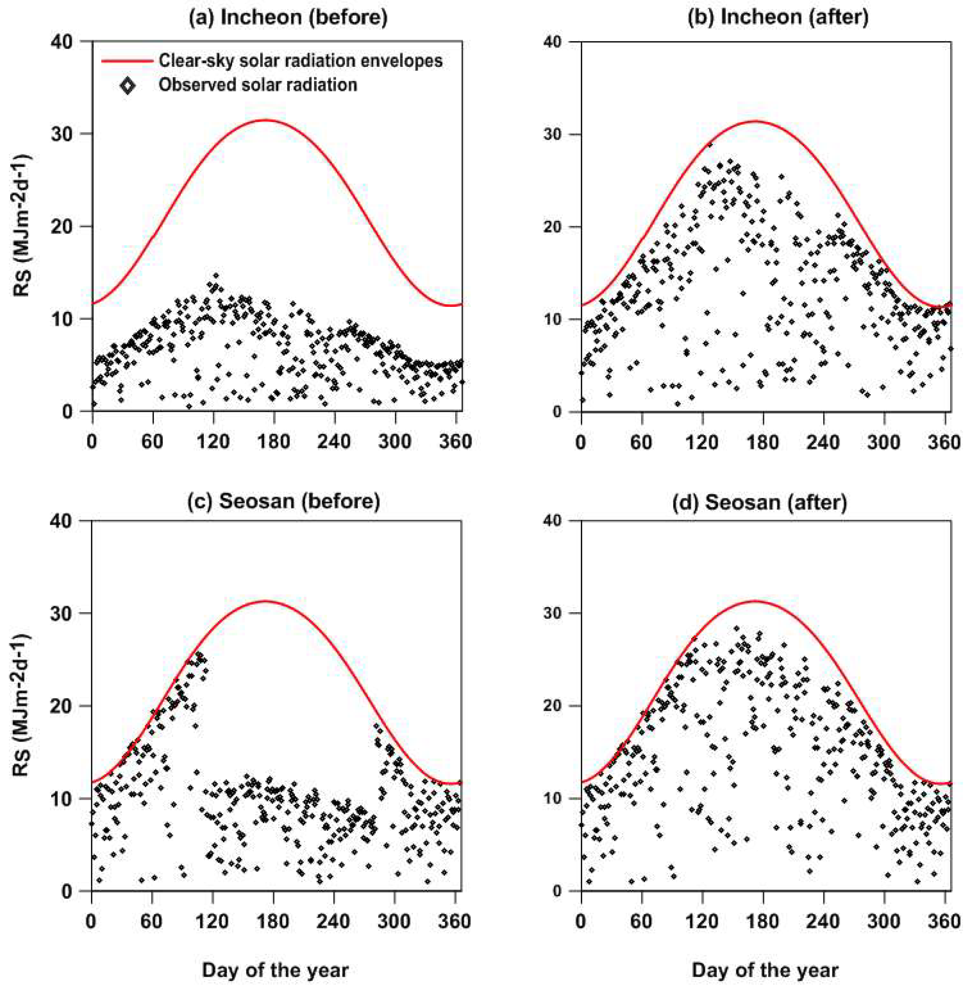
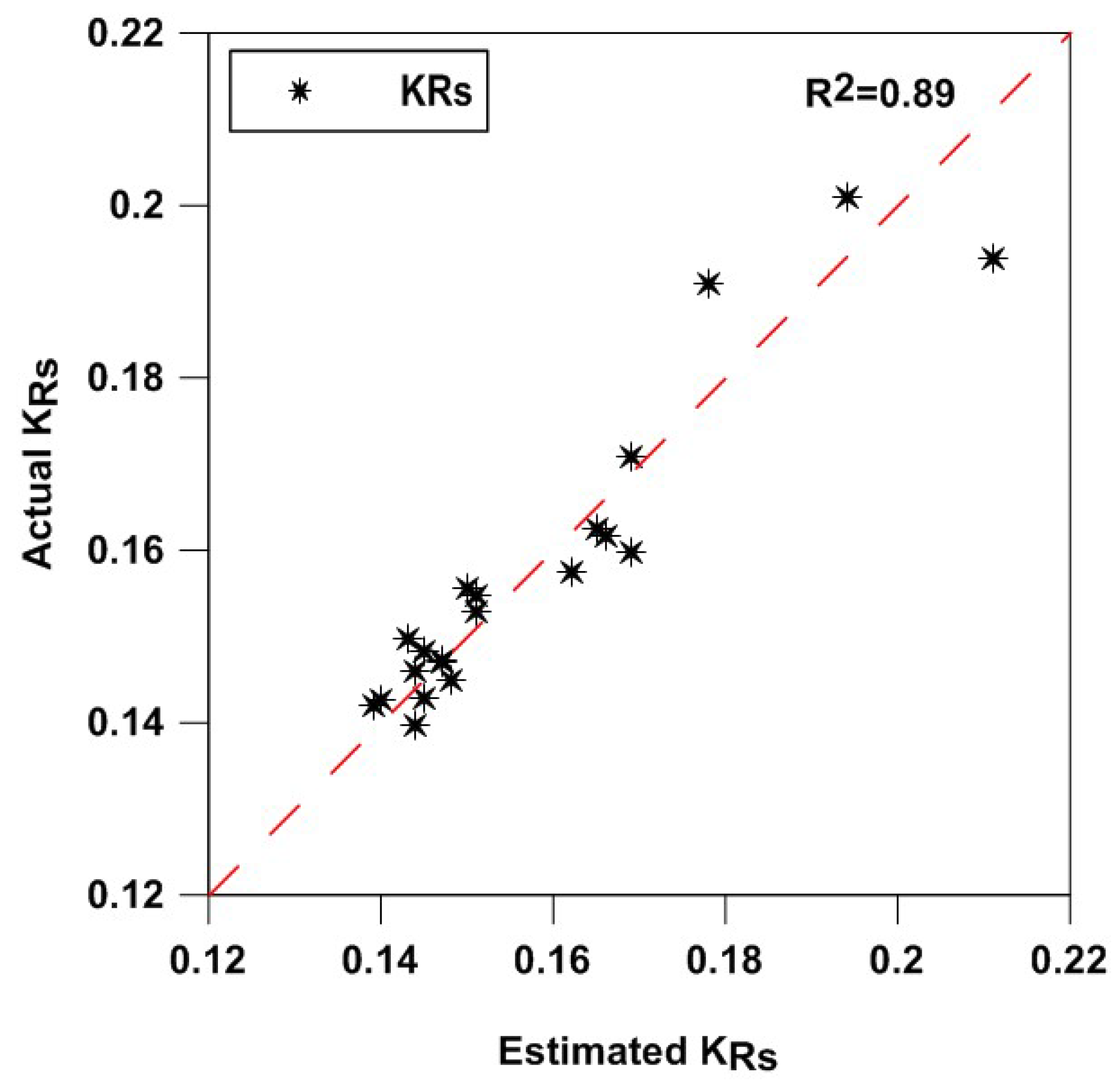
2.2. Estimation of Solar Radiation

Solar radiation, or total sunshine hours, is one of the inputs used in the FAO PM method to estimate ET_o. However, when solar-radiation or sunshine-duration data are unavailable, FAO 56 recommends using Hargreaves’ radiation formula to estimate solar radiation. Hargreaves’ radiation formula is calibrated and validated for various stations in different climate conditions. This formula, proposed by Reference [21], is expressed as follows:

$$R_s= K_{Rs} \sqrt{\left(TD\right)} R_a$$

(3)

where $R_s$ is the solar radiation (MJ m⁻² day⁻¹); TD is the diurnal temperature, which is the difference between the maximum temperature ($T_{max}$) and the minimum temperature ($T_{min}$) (°C); K_Rs is the adjustment coefficient; and R_a is the extraterrestrial radiation (MJ m⁻² day⁻¹), which varies throughout the day of the year and latitude.

Hargreaves (1994) [22] suggested values of $K_{Rs}=0.16$ for inland areas and $K_{Rs}=0.19$ for coastal regions. However, other studies have recommended calibrating $K_{Rs}$ regionally to obtain an accurate estimation of solar radiation using long-term mean temperature ($T_{mean}$) and diurnal temperature (TD) [23,24,25]. In the regional calibration of $K_{Rs}$, $K_{Rs}$ values are calculated using the ratio of the daily $R_s$ to $R_a$ and the square root of TD for each meteorological station. Then, the different relations for $K_{Rs}$ are determined using multiple regression with the long-term mean $T_{mean}$ and TD ($\frac{T_{mean}}{TD})$, station elevation (EL), and latitude (φ) as the independent variables. After statistical analysis, the selected relation for $K_{Rs}$ was applied to estimate $R_{\mathrm{s}}$ using Equation (3).

2.3. Trend-Analysis Method

Parametric T-tests [26] and nonparametric Mann–Kendall trend tests [27,28,29] were used to determine the trends in the seasonal and annual ${\mathrm{ET}}_{\mathrm{o}}$ and components of the FAO PM method (i.e., ${\mathrm{EN}}_{\mathrm{o}}$ and ${\mathrm{AE}}_{\mathrm{o}})$.

2.3.1. Parametric T-Test

The T-test is a parametric test considering the assumption that data are normally distributed and uses a statistical technique for detecting trends in a time series by fitting a linear equation to observations. The estimated equation uses a linear relationship between X as an independent variable and Y as a dependent variable, and is written as follows:

$$Y=A+B\times X$$

(4)

where $A$ and $B$ denote the intercept and the slope of the regression line, respectively. Positive slope A represents an upward trend and a negative slope indicates a downward trend in a time series. The T-tests apply the hypothesis test on the standard slope coefficient, and the result defines as $T_o$ and is calculated with the following equation:

$$T_o=\frac{B_1}{SE}$$

(5)

where $B_1$ is the standard slope of the regression line and $SE$ is the standard error of the slope. $SE$ is calculated as follows:

$$SE=\frac{\sqrt{{{\displaystyle \sum }}_{i=1}^n{\left(y_i-\overline{y}\right)}^2/n-2}}{\sqrt{{{\displaystyle \sum }}_{i=1}^n{\left(x_i-\overline{x}\right)}^2}}$$

(6)

where, $x_i$ is an independent variable and $y_i$ is an independent variable in the time series. $\overline{x}$ is the average of $x_i$ and $\overline{y}$ is the average of $y_i$ in the time series, and n is the number of observed data. $T_o$ has a t distribution with n—2 degrees of freedom, where n is the total number of observations. Null hypothesis has no significant trend for $T_o$ if

$$-t_{\frac{\alpha }{2},n-2}<T_o<t_{\frac{\alpha }{2},n-2}$$

(7)

where $t_{\frac{\alpha }{2},n-2}$ and $-t_{\frac{\alpha }{2},n-2}$ represent the standard normal deviates and $\alpha$ determines the level of significance. In this test, 5% and 10% significance levels are considered.

2.3.2. Nonparametric Mann–Kendall test

The Mann–Kendall (MK) test is a nonparametric test used to analyze the null hypothesis of no change in the mean of a series (no trend) against the alternative hypothesis of an increase or decrease over time (existence of a trend) [30]. This method is frequently used to determine trends in hydrological variables. Kendall’s statistic S is obtained using the following equations:

$$S={\displaystyle \sum }_{i=1}^{n-1}{\displaystyle \sum }_{j=i-1}^{n}Sgn\left(X_j-X_i\right)$$

(8)

$$\mathrm{Sgn}\left(X_j-X_i\right)=\{\begin{array}{c}+1 if\left(X_j-X_i\right)>0\\ 0 if\left(X_j-X_i\right)=0\\ -1 if\left(X_j-X_i\right)<0 \end{array}$$

(9)

where n is the number of observations, X_j and X_i are sequential data (j > i), and Sgn ($X_j-X_i$) is a sign function that extracts the sign of $X_j-X_i$. Statistic S has normal distribution with zero mean and variance and is computed as

$$Var \left(S\right)= \frac{\left[n\left(n-1\right)\left(2n+5\right)-{{\displaystyle \sum }}_{i=1}^{m}t\left(t-1\right)\left(2t+5\right)\right]}{18}$$

(10)

where m is the number of ties, t is the size of the ith tie, and Σ is the summation of all ties. MK statistic Z is estimated as follows:

$$Z=\{\begin{array}{c}\frac{S-1}{\sqrt{Var \left(S\right)}} if S>0\\ 0 if S=0\\ \frac{S+1}{\sqrt{Var \left(S\right)}} if S<0 \end{array}$$

(11)

where Z is the standard normal variable, with positive values of Z indicating increasing trends, whereas negative values indicate decreasing trends. The null hypothesis H_o that Z has no significant trend is accepted if $-Z_{1-\frac{\alpha }{2}}\le Z\le Z_{1-\frac{\alpha }{2}}$, where α is the significance level for the test (5% and 10% significance levels) and +$Z_{1-\frac{\alpha }{2}}$ and $-Z_{1-\frac{\alpha }{2}}$ are the critical values for the two-sided hypothesis. The slope of the trends in the nonparametric MK test can be calculated as follows:

$$\beta =Median \left[\frac{X_j-X_i}{j-i}\right] for all i<j$$

(12)

where $X_j$ and $X_i$ are sequential data (j > i) and β is Theil–Sen’s estimator, which is a robust estimate of the trend magnitude in the MK test. A positive Theil–Sen slope indicates an increasing trend and a negative slope represents a decreasing trend in a time series.

2.4. Impact of Serial Correlation in a Time Series

The parametric T-test and MK test are designed for serially independent series. Therefore, the presence of incorrect rejection of the null hypothesis when there is no trend (Type I error) is correct only when the data are independent. As serial correlation increases, the variance of the test statistic and the rejection rate of the null hypothesis increase, specifically when there is a positive serial correlation [30,31]. In this study, the prewhitening approaches proposed by von Storch and Navarra [32] were used to eliminate the effect of serial correlation by removing the lag-one autoregressive component $\left(r_1\right)$ of the series with serial correlation before applying trend tests. To this end, $r_1$ was computed and compared to the 95% confidence limits. If $r_1$ ranged between $\frac{-1-1.96\sqrt{n-2}}{n-1}\le r_1\le \frac{-1+1.96\sqrt{n-2}}{n-1}$, $r_1$ was not significant; otherwise, $r_1$is significant ($n$ is the number of data). The trend tests are applied to the original time series $\left(x_1,x_2,\dots ,x_n\right)$ if $r_1$ is not significant. However, if $r_1$ is significant, then the time series should be prewhitened as $\left(x_2-r_1{x}_1,x_3-r_1{x}_2,\dots ,x_n-r_1{x}_{n-1}\right)$ to remove the effect of serial correlation prior to application of the trend tests [31,33].

3. Study Area and Data

The Korean Peninsula is in northeastern Asia and is divided into two parts: South Korea (SK) and North Korea (NK). Figure 1 shows the spatial distribution of stations (name and code) of topographic and land-cover characteristics of the study area. The Korean Peninsula is connected to the northeastern part of mainland China and is surrounded by oceans along the eastern, western, and southern coasts. The peninsula is mountainous in the northern and eastern parts and has well-developed plains in the western and southern parts. The climate of the peninsula is affected by the East Asian monsoon in summer and typhoons in autumn. Nearly two-thirds of the annual rainfall occurs during the flooding season in the summer months [34]. Winters are cold, with typical January temperatures below freezing and minimal precipitation and little snow accumulation outside of the mountainous areas. However, climate differs dramatically from North to South Korea. The northern regions have a colder climate in the more mountainous area (in the north and east), while the southern regions have a warm and wet climate in the flat plains of the southern and western peninsula. Monthly average rainfall is approximately 112.5 mm in SK and 74.5 mm in NK. Mean annual temperature is 13.1 °C in SK, from 1.2 °C in winter to 24.1 °C in summer, and 9.0 °C in NK, from –4.7 °C in winter to 21.5 °C in summer.

The detection of ${\mathrm{ET}}_{\mathrm{o}}$ trends requires the use of long-term meteorological data, including the daily observed $R_s$,$T_{max}$, $T_{min}$, dew-point temperature $(T_{dew})$, and wind speed $\left(W_s\right)$. Daily meteorological data from 21 meteorological stations in SK and 27 stations in NK were collected from the Korea Meteorological Administration (https://data.kma.go.kr) within a sufficient meteorological time period (1980–2017). Statistics for the observed daily $R_s$ are available for the 21 weather stations in SK but not for those in NK. The spatial distribution of the stations in SK and NK is shown in Figure 1.

The data quality and integrity assessments were performed using the procedures explained by Reference [6] prior to the analysis. The missing data were filled with averaged values from the neighboring sites using an inverse-distance weighting method [35]. The numbers of missing data for each parameter of stations in SK and NK are provided in Table S2. For the quality check for temperature, the observed $T_{max}$ and $T_{min}$ data were compared against the long-term temperature extremes for each year [24]. To evaluate the integrity of solar-radiation data, the observed solar-radiation data of each station were compared with the clear-sky solar-radiation envelope ($R_{so}$) for each year. $R_{so}$ is a function of a day of the year, latitude, and elevation. The calculated $R_{so}$ can be plotted as an upper envelope of observed Rs. This method is especially useful for areas with high air pollution or airborne dust without clear skies. In these regions, there were differences between the measured $R_s$ and calculated $R_{so}$, and $R_s$ was significantly below or above the computed $R_{so}$. This issue was further investigated by using multiplicative factor (${\left(R_s\right)}_{cor}=a.R_s),$ additive factor (${\left(R_s\right)}_{cor}=a+R_s),$or a combination of these variables to force the measured R_S to reach the computed $R_{so}$ (where a is the corrective factor). Additional explanation about the integrity of solar-radiation data using clear-sky comparisons can be found in FAO 56 [6,24,36]. There were differences between $R_s$and $R_{so}$ for some years at stations in SK. These mismatches were found and modified for all stations in SK. Figure 2 shows the time series of solar radiation before and after this prescreening for the Incheon station in 1980 and Seaosan station in 1982.

4. Results and Discussion.

4.1. Regional Calibration of $K_{Rs}$ and Estimation of Solar Radiation

Due to the lack of solar-radiation data in NK, $R_s$ was estimated based on Hargreaves’ formula and the regionally calibrated formula for $K_{Rs}$. The different relationships were determined by multiregression of long-term mean values of $\frac{T_{mean}}{TD}$, EL, and $\phi$ as the independent variables and station values of $K_{Rs}$ as the dependent variable. The following equation was selected as the best model after statistical analysis:

$$K_{Rs}=0.032\frac{T_{mean}}{TD}+ \left(2.29\times {10}^{-5}\mathrm{EL}\right)+0.105$$

(13)

Figure 3 depicts the actual $K_{Rs}$ against the computed $K_{Rs}$ using Equation (13) in SK. The estimated $K_{Rs}$ values are well-correlated with the calculated values, with a high correlation coefficient (R² = 0.89) and small root-mean-square error (RMSE = 0.007). Using the $K_{Rs}$ values for all stations in SK and NK, $R_s$ was estimated using Hargreaves’ formula (Equation (3)) for all stations in SK and NK.

Table 1. Statistical analysis for comparison of daily observed and calculated solar-radiation data for 21 stations of South Korea (SK).

Station Code	Station Name	R2	Root-Mean-Square Error (RMSE)
100	Daegwalryeong	0.87	3.00
101	Chuncheon	0.85	3.07
105	Gangnung	0.86	3.10
108	Seoul	0.84	3.57
112	Incheon	0.82	3.73
114	Wonju	0.66	4.96
129	Seosan	0.85	4.11
131	Cheongju	0.83	3.49
133	Daejeon	0.86	2.68
135	Chupungyong	0.81	3.53
136	Andong	0.84	2.98
138	Pohang	0.85	3.18
143	Daegu	0.89	2.71
146	Jeonju	0.88	2.81
156	Gwangju	0.88	2.70
159	Busan	0.86	3.17
165	Mokpo	0.89	2.59
184	Jeju	0.92	2.67
185	Gosan	0.87	2.84
169	Heuksando	0.90	1.78
192	Jinju	0.88	2.56

shows the statistical analysis for the comparison of observed and calculated daily solar-radiation data for 21 stations in SK. The results show good agreement between observed and estimated solar-radiation data in SK. However, because $K_{Rs}$ was determined using regional calibration data in SK, there is uncertainty in the estimated $R_s$ in NK.

4.2. Estimation of $E{T}_o$ Using the Penman–Monteith Method

The time series of the annual ${\mathrm{ET}}_{\mathrm{o}}$ for 27 stations in NK and 21 stations in SK are illustrated as a box-and-whisker plot in Figure 4a and b, respectively. In NK, the maximum and minimum estimated ${\mathrm{ET}}_{\mathrm{o}}$ values were at Huicheon station (1005.5 mm) and Seonbong station (660.3 mm), respectively. In SK, the maximum estimated ${\mathrm{ET}}_{\mathrm{o}}$ was 1192.8 mm for Daegu station, whereas the minimum was 826 mm for Daegwalryeong station, indicating that the mean annual ${\mathrm{ET}}_{\mathrm{o}}$ in SK is higher than that in NK.

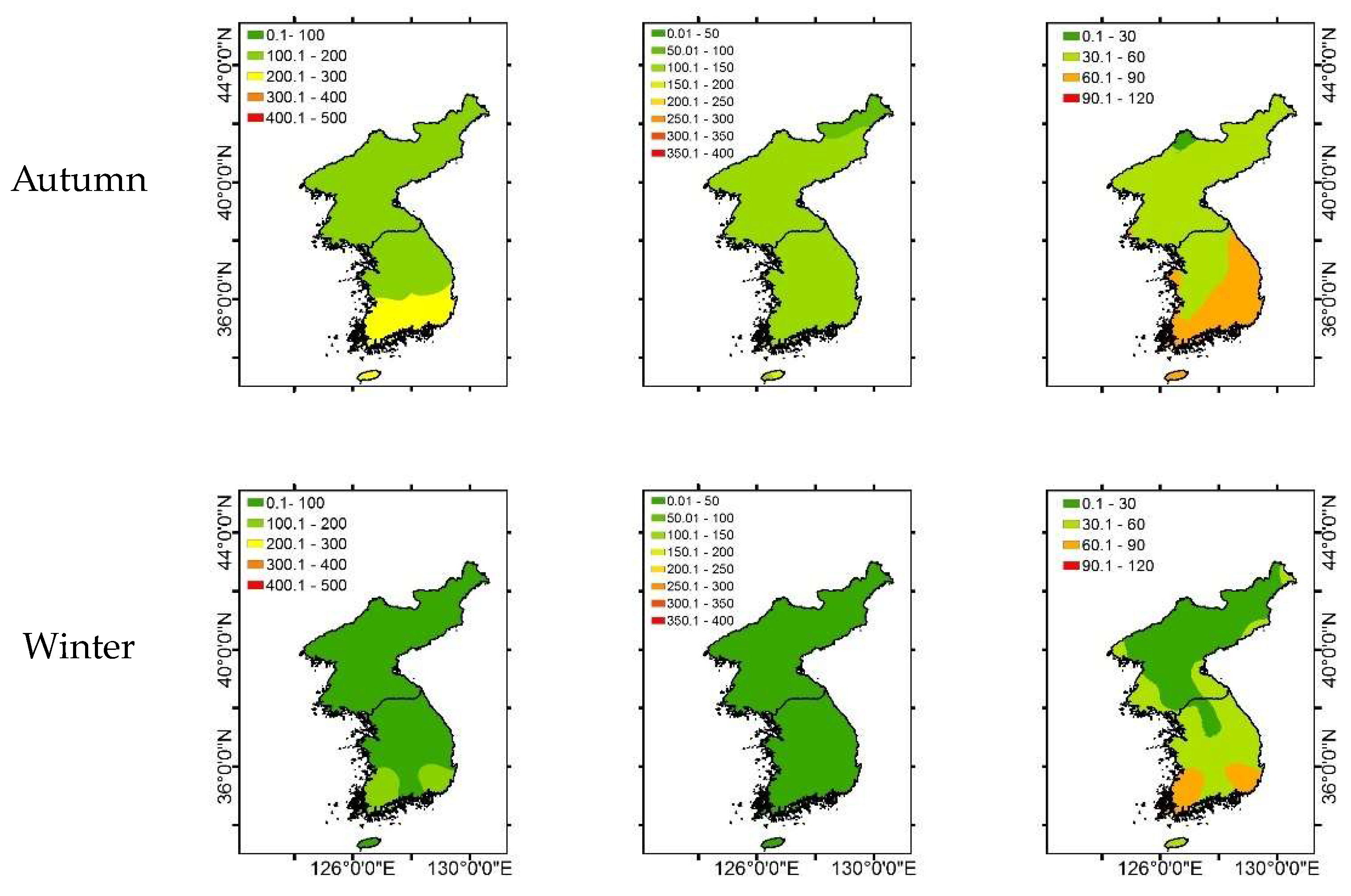
4.3. Spatial Distribution of Mean Annual and Seasonal $E{T}_o$, $E{N}_o$, and $A{E}_o$

The Kriging method was used to interpolate the mean annual and seasonal ${\mathrm{ET}}_{\mathrm{o}}$, ${\mathrm{EN}}_{\mathrm{o}}$, and ${\mathrm{AE}}_{\mathrm{o}}$ over the Korean Peninsula by including the data of all stations in SK and NK. The Kriging method is widely used for spatial analysis by using geographic information systems (GIS). This method applies the distance-weighting approach to interpolating the data by including information from specific locations [37]. The spatial distribution pattern of the mean annual ${\mathrm{ET}}_{\mathrm{o}}$ averaged from 1980 to 2017 is shown in Figure 5, which reflects the combined effect of meteorological variables and topographic characteristics across the Korean Peninsula. The annual ${\mathrm{ET}}_{\mathrm{o}}$ variation exhibits a clear spatial pattern (southward increase), ranging from 705 $\mathrm{mm}/\mathrm{year}$ to 1195 $\mathrm{mm}/\mathrm{year}$ over the entire basin. A lower ${\mathrm{ET}}_{\mathrm{o}}$ is present in the northeast, while higher values are found in the southeast of the Korean Peninsula.

The spatial distribution of mean annual ${\mathrm{EN}}_{\mathrm{o}}$ and ${\mathrm{AE}}_{\mathrm{o}}$ show that there is a distinct pattern of minimum values in the northern area and maximum values in the southern area of the Korean Peninsula with different directions of variation. The spatial distribution of ${\mathrm{EN}}_{\mathrm{o}}$ decreases from the southwest to the northeast direction of the Korean Peninsula, while regarding the ${\mathrm{AE}}_{\mathrm{o}}$, the maximum was established in the southeastward direction and the minimum in the northward. This pattern occurs because the energy term mainly affects the $R_s$ and T. $R_{\mathrm{s}}$ is different based on the latitude due to the differences in the position of the sun [6], and it is higher near the equatorial region than the polar region. Thus, higher $R_s$ were observed in the southern part (higher latitude) of the Korean Peninsula than the northern part (lower latitude). Additionally, T in North Korea mainly affects the propagation of Siberian cold weather, and the movement of this cold stream from Siberia to North Korea produces temperature drops in the region. However, T in South Korea is higher, which is mostly affected by the subtropical warm current. Therefore, the higher magnitude of $R_{\mathrm{s}}$ and T in South Korea causes a higher value of ${\mathrm{EN}}_{\mathrm{o}}$ in SK than NK. ${\mathrm{AE}}_{\mathrm{o}}$ primarily affects the relative humidity and wind speed. The intense value of relative humidity and wind speed in the southern part causes higher ${\mathrm{AE}}_{\mathrm{o}}$ in SK relative to NK. In general, the higher value of ${\mathrm{EN}}_{\mathrm{o}}$ and ${\mathrm{AE}}_{\mathrm{o}}$ in SK than NK results in higher ${\mathrm{ET}}_{\mathrm{o}}$ in SK.

Moreover, the seasonal spatial distribution of ${\mathrm{ET}}_{\mathrm{o}}$ shows that the highest amount of ${\mathrm{ET}}_{\mathrm{o}}$ occurs in the summer and then in spring, while winter has the lowest value of ${\mathrm{ET}}_{\mathrm{o}}$. This pattern exists due to the high amount of ${\mathrm{EN}}_{\mathrm{o}}$ in the summer and the seasonal spatial distribution of ${\mathrm{EN}}_{\mathrm{o}}$. Furthermore, the comparison of the spatial distribution of ${\mathrm{ET}}_{\mathrm{o}}$ with ${\mathrm{EN}}_{\mathrm{o}}$ and ${\mathrm{AE}}_{\mathrm{o}}$ in different seasons shows that ${\mathrm{ET}}_{\mathrm{o}}$ in spring and summer is mostly affected by ${\mathrm{EN}}_{\mathrm{o}}$, whereas in autumn and winter it is mostly caused by ${\mathrm{AE}}_{\mathrm{o}}$. This finding indicates that ${\mathrm{ET}}_{\mathrm{o}}$ in spring and summer has a stronger effect resulting from the superimposed effect of $R_s$ and T in autumn and winter by the combined influence of RH and WS.

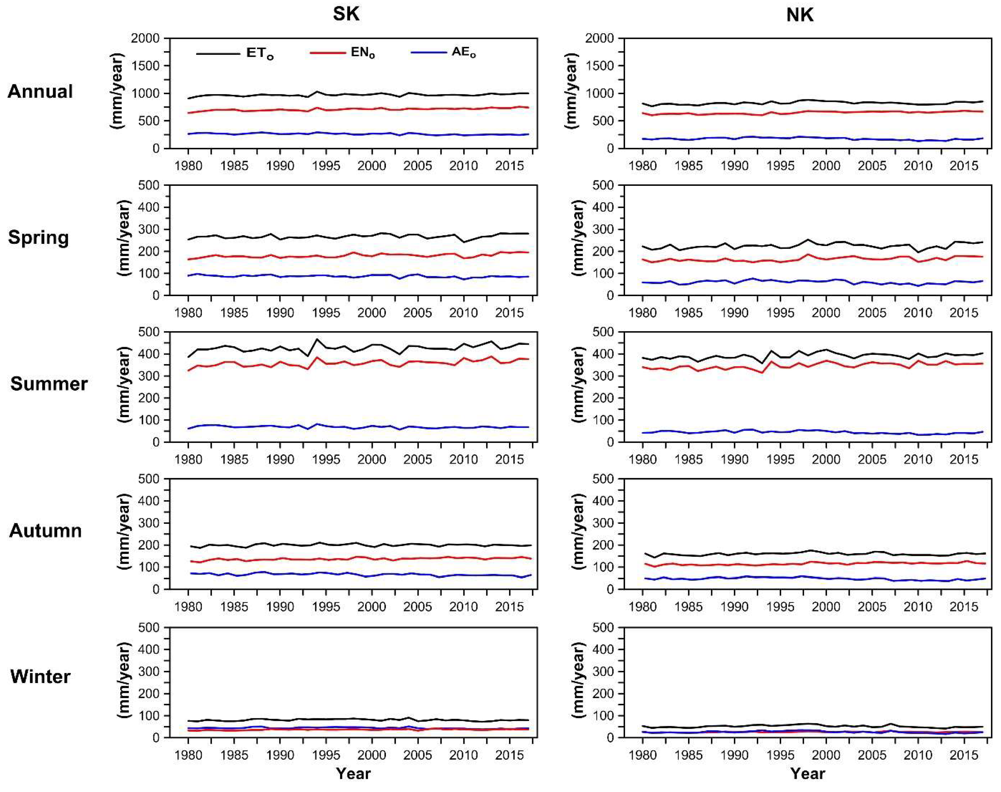
4.4. Differences in the Mean Annual and Seasonal $E{T}_o$, $E{N}_o$, and $A{E}_o$ between SK and NK

The time series of seasonal and annual ${\mathrm{ET}}_{\mathrm{o}}$, ${\mathrm{EN}}_{\mathrm{o}}$, and ${\mathrm{AE}}_{\mathrm{o}}$ from 1980 to 2017 averaged over the entire catchment in SK and NK are graphically presented in Figure 6, and the comparison of the results is reported in

Table 2. Mean seasonal and annual ${\mathrm{ET}}_{\mathrm{o}}$, ${\mathrm{EN}}_{\mathrm{o}}$, and ${\mathrm{AE}}_{\mathrm{o}}$ from 1980 to 2017 and ratios with ${\mathrm{ET}}_{\mathrm{o}}.$

Period	ETo	Annual ETo	ENo	AEo	ENo/ETo	AEo/ETo
	(mm/year)	(%)	(mm/year)	(mm/year)	(%)	(%)
South Korea
Spring	267.6	27.6	180.5	87.1	67.4	32.6
Summer	426.9	44.0	358.0	68.9	83.9	16.1
Autumn	196.0	20.2	133.3	62.8	68.0	32.0
Winter	80.6	8.3	36.6	43.9	45.5	54.5
Annual	971.2	100.0	708.4	262.7	72.9	27.1
North Korea
Spring	224.9	27.3	164.4	60.5	73.1	26.9
Summer	391.1	47.5	346.3	44.8	88.6	11.4
Autumn	155.9	18.9	111.4	44.4	71.5	28.5
Winter	51.7	6.3	25.9	25.8	50.1	49.9
Annual	823.5	100.0	648.0	175.5	78.7	21.3

. The mean annual ${\mathrm{ET}}_{\mathrm{o}}$ in SK is 971.2 mm/year, whereas that for NK is 823.5 mm/year, which indicates that the mean annual ${\mathrm{ET}}_{\mathrm{o}}$ in SK is 18% higher than that in NK over the 37-year period. In addition, the annual ${\mathrm{EN}}_{\mathrm{o}}$ and ${\mathrm{AE}}_{\mathrm{o}}$ terms are 708.4 and 262.7 mm/year in SK and 648.0 and 175.5 mm/year in NK, respectively. It follows that mean areal ${\mathrm{EN}}_{\mathrm{o}}$ and ${\mathrm{AE}}_{\mathrm{o}}$ are higher, at 9.3% and 49.7%, respectively, in SK than in NK.

The most seasonal ${\mathrm{ET}}_{\mathrm{o}}$ occurs in summer, which constitutes 44% and 47.5% of the total ${\mathrm{ET}}_{\mathrm{o}}$ in SK and NK, respectively (Table 2). The lowest ${\mathrm{ET}}_{\mathrm{o}}$ occurs in winter in both SK and NK (8.3% in SK and 6.3% in NK). However, the annual ${\mathrm{ET}}_{\mathrm{o}}$ exhibits similar ratios in spring and autumn.

To understand which of the components of ${\mathrm{ET}}_{\mathrm{o}}$ (i.e., ${\mathrm{EN}}_{\mathrm{o}}$ and ${\mathrm{AE}}_{\mathrm{o}}$) result in higher ${\mathrm{ET}}_{\mathrm{o}}$ in SK than NK, the percentages of mean ${\mathrm{EN}}_{\mathrm{o}}$ and ${\mathrm{AE}}_{\mathrm{o}}$ were compared to the mean ${\mathrm{ET}}_{\mathrm{o}}$ for each season (see Table 2). The results reveal that spring and autumn have similar percentages of ${\mathrm{EN}}_{\mathrm{o}}$ and ${\mathrm{AE}}_{\mathrm{o}}$ in SK and NK, while the energy term $\left({\mathrm{EN}}_{\mathrm{o}}\right)$ constitutes almost 70% and the aerodynamic term covers $\left({\mathrm{AE}}_{\mathrm{o}}\right)$ 30% of the total ${\mathrm{ET}}_{\mathrm{o}}$ on the Korean Peninsula. The ${\mathrm{EN}}_{\mathrm{o}}$ in summer has the greatest impact on the ${\mathrm{ET}}_{\mathrm{o}}$ when compared to the other seasons and contains approximately 85% of the total ${\mathrm{ET}}_{\mathrm{o}}$ in SK and NK. Furthermore, in winter, ${\mathrm{EN}}_{\mathrm{o}}$ and ${\mathrm{AE}}_{\mathrm{o}}$ have almost the same portion of ${\mathrm{ET}}_{\mathrm{o}}$(approximately 50%). These results indicate that the ${\mathrm{EN}}_{\mathrm{o}}$ term plays an important role in ${\mathrm{ET}}_{\mathrm{o}}$ during the spring, summer, and autumn, while in the winter, both terms contribute equally to the amount of ${\mathrm{ET}}_{\mathrm{o}}$.

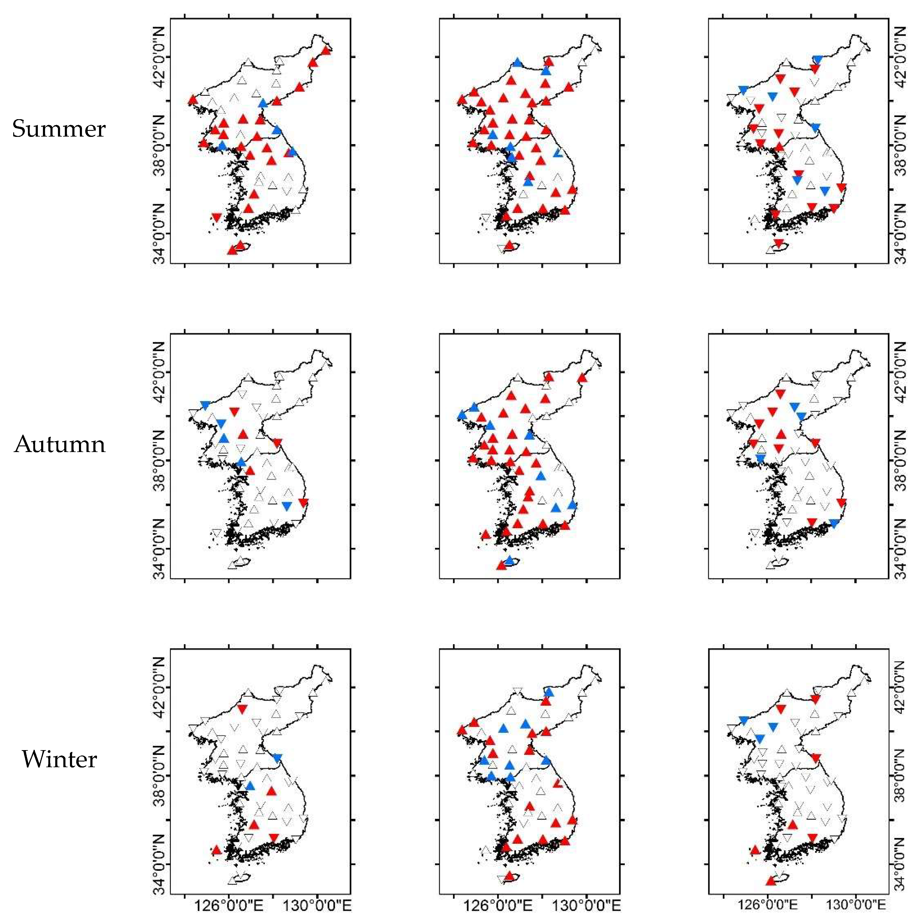
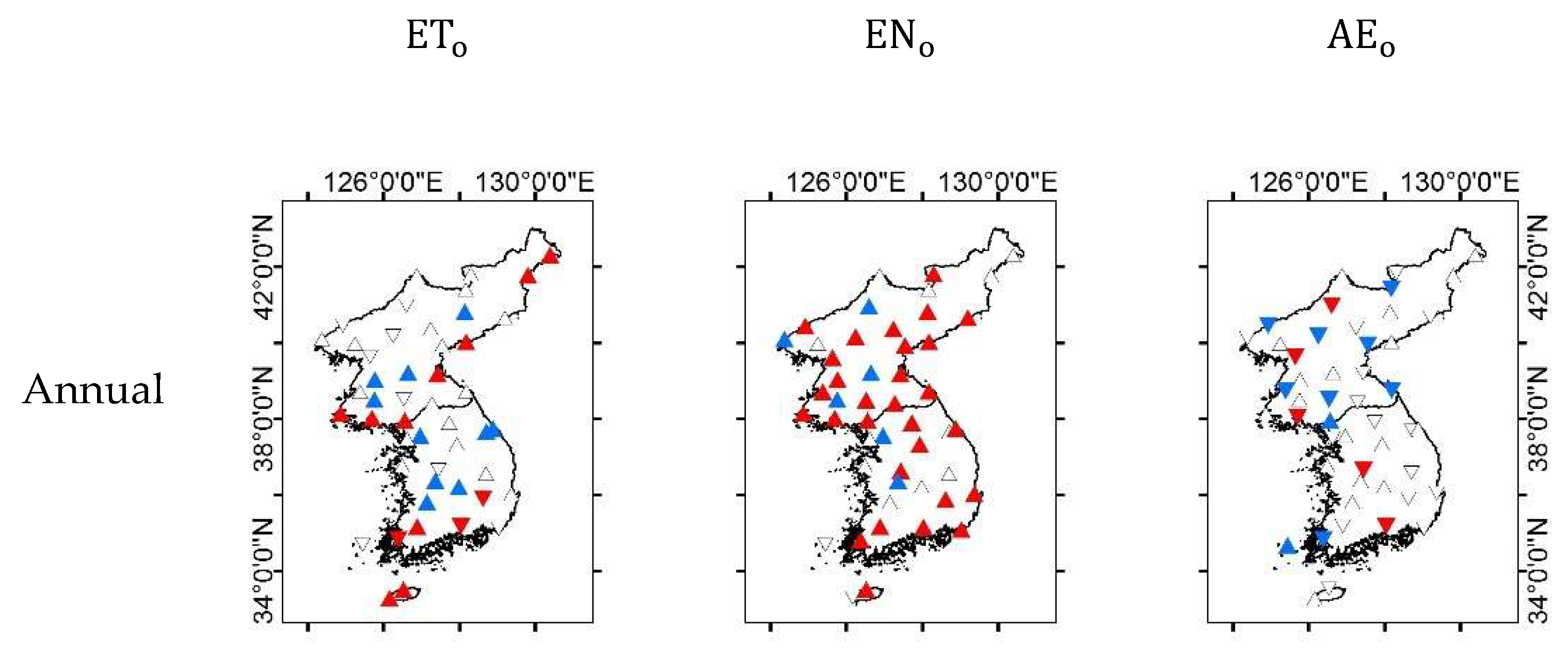
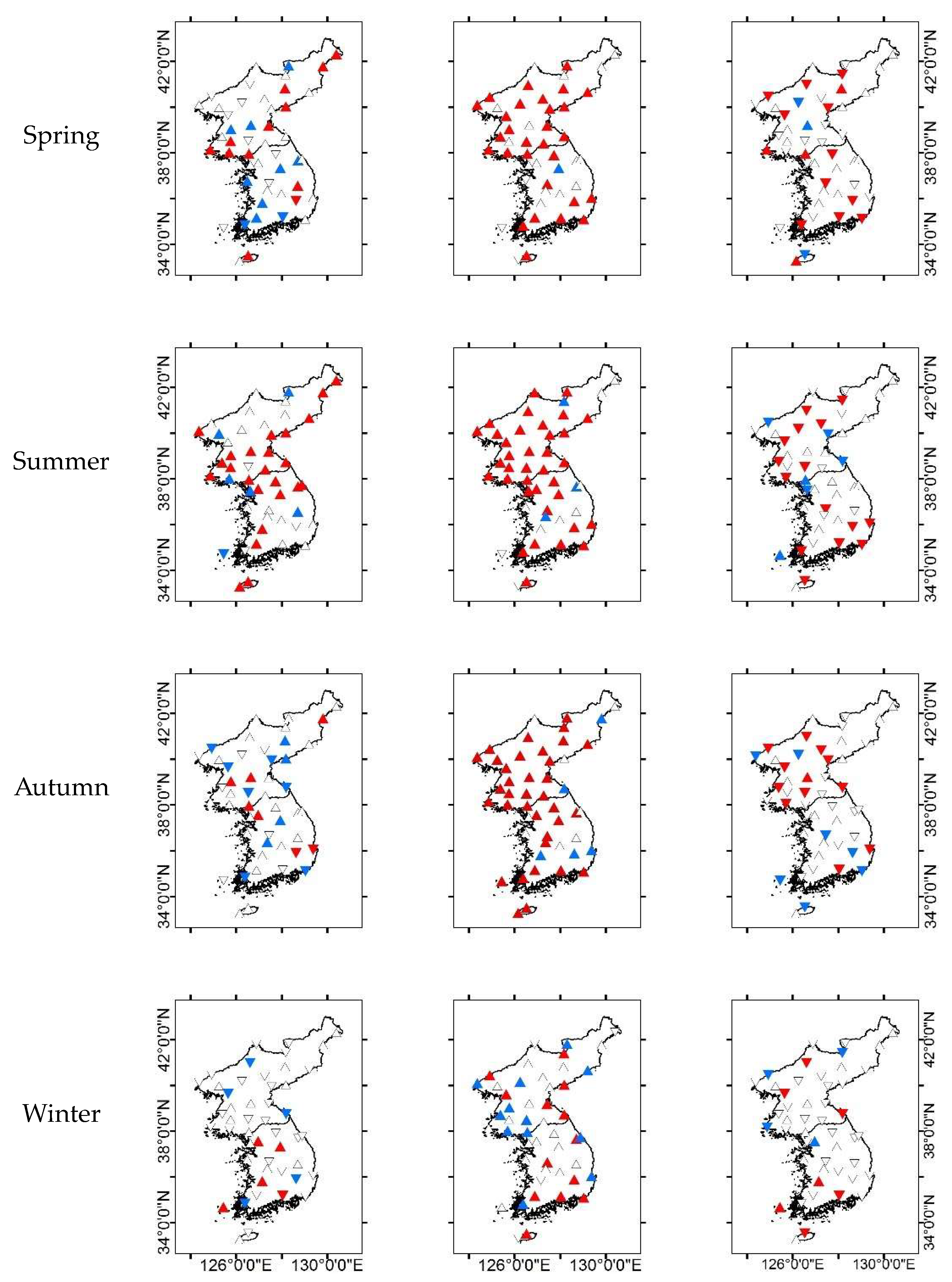
4.5. Spatial Variation of Annual and Seasonal $E{T}_o$, $E{N}_o$, and $A{E}_o$ Trends

The results of prewhitening for ${\mathrm{ET}}_{\mathrm{o}}$, ${\mathrm{EN}}_{\mathrm{o}}$, and ${\mathrm{AE}}_{\mathrm{o}}$ on an annual scale are reported in Tables S3–S5 as supplementary documents. The spatial distributions of stations in SK and NK from 1980 to 2017 with significant increasing or decreasing trends according to the MK test are presented in Figure 7. As shown, 43% of stations in SK reveal significant increasing trends, and 14% show significant decreasing trends in annual ${\mathrm{ET}}_{\mathrm{o}}$. The significant decreasing trend in SK is located in the southeastern area of the Korean Peninsula. However, 22% of stations in NK detected significant increasing trends, mainly located in the coastal areas, while 4% of the stations revealed significant decreasing trends. The annual spatial distribution of ${\mathrm{EN}}_{\mathrm{o}}$ showed that 66% of stations in SK, as well as NK, detected significant increasing trends, while no station showed significant decreasing trends for annual energy trends. In contrast, for ${\mathrm{AE}}_{\mathrm{o}}$, significant decreasing trends were detected at 19% of stations in SK and 33% stations in NK; however, there were no significant increasing trends for this variable. These results indicated that significant increasing trends on the Korean Peninsula are caused by the significant increasing trends in the energy term. As described above, the ${\mathrm{EN}}_{\mathrm{o}}$ is primarily related to solar radiation and temperature. It follows that the trends of $R_{\mathrm{s}}$ and T were increased on the Korean Peninsula. Similar results were also found using the T-test, and the results are shown in Figure 8.

The results showed that ${\mathrm{ET}}_{\mathrm{o}}$ increased more significantly on the plains than in the mountainous areas. ${\mathrm{EN}}_{\mathrm{o}}$ increased in both areas, while ${\mathrm{AE}}_{\mathrm{o}}$ decreased more significantly in the plains than in the mountainous areas.

In addition, the spatial distributions of the seasonal trends in ${\mathrm{ET}}_{\mathrm{o}}$ and its components were investigated. The spatial trends of ${\mathrm{ET}}_{\mathrm{o}}$ in spring revealed significant increasing trends for 29% and 44% of stations in SK and NK, respectively. Additionally, in summer, 33% of stations in SK and 59% of stations in NK detected significant increasing trends. This finding indicates that there is a more intense significant trend during spring and summer in NK. Moreover, the spatial distribution of ${\mathrm{ET}}_{\mathrm{o}}$ during autumn and winter revealed both significant upward and downward trends on the Korean Peninsula. Regarding the ${\mathrm{EN}}_{\mathrm{o}}$, only significant increasing trends were detected for stations, and no station detected a significant downward trend. In contrast, almost all significant detected trends for ${\mathrm{AE}}_{\mathrm{o}}$ are decreasing for all seasons over the Korean Peninsula. These opposite trends in ${\mathrm{EN}}_{\mathrm{o}}$ and ${\mathrm{AE}}_{\mathrm{o}}$caused the mitigation of the significant trends of ${\mathrm{ET}}_{\mathrm{o}}$. Furthermore, the stronger significant upward trends of energy terms led to significant increasing trends of ${\mathrm{ET}}_{\mathrm{o}}$ on the Korean Peninsula.

4.6. Difference in Trends of Mean Annual and Seasonal $E{T}_o$, $E{N}_o$, and $A{E}_o$ in SK and NK

The time series of ${\mathrm{ET}}_{\mathrm{o}}$, ${\mathrm{EN}}_{\mathrm{o}}$, and ${\mathrm{AE}}_{\mathrm{o}}$ from 1980 to 2017 were averaged over the entire SK and NK using the kriging method. Then, the parametric T-test and nonparametric MK test were performed to detect the trends of ${\mathrm{ET}}_{\mathrm{o}}$ and its components in the seasonal and annual scales, and the results are reported in

Table 3. Statistical trends in the seasonal and annual ${\mathrm{ET}}_{\mathrm{o}}$, ${\mathrm{EN}}_{\mathrm{o}}$, and ${\mathrm{AE}}_{\mathrm{o}}$ from 1980 to 2017.

Period	South Korea				North Korea
	Parametric T-Test		Nonparametric MK Test		Parametric T-Test		Nonparametric MK Test
	T	B	Z	β	T	B	Z	β
ETo
Spring	$\underset{\_}{\underset{\_}{1.67}}$	0.26	2.03	0.28	$\underset{\_}{\underset{\_}{1.94}}$	0.31	$\underset{\_}{\underset{\_}{2.09}}$	0.35
Summer	2.18	0.34	2.26	0.45	2.51	0.39	$\underset{\_}{\underset{\_}{2.63}}$	0.40
Autumn	0.59	0.09	0.04	–0.03	0.66	0.10	0.16	–0.03
Winter	–0.53	–0.08	–0.46	–0.06	–0.32	–0.05	–0.21	–0.07
Annual	2.42	0.38	2.69	0.60	1.30	0.21	0.98	0.08
ENo
Spring	2.23	0.35	$\underset{\_}{\underset{\_}{2.33}}$	0.23	2.42	0.38	$\underset{\_}{\underset{\_}{2.77}}$	0.33
Summer	3.47	0.55	$\underset{\_}{\underset{\_}{3.39}}$	0.65	2.90	0.46	$\underset{\_}{\underset{\_}{2.64}}$	0.54
Autumn	2.44	0.38	$\underset{\_}{\underset{\_}{2.03}}$	0.15	2.54	0.40	$\underset{\_}{\underset{\_}{2.08}}$	0.16
Winter	1.97	0.31	$\underset{\_}{\underset{\_}{2.15}}$	0.07	$\underset{\_}{\underset{\_}{1.66}}$	0.26	$\underset{\_}{\underset{\_}{1.96}}$	0.05
Annual	2.63	0.42	$\underset{\_}{\underset{\_}{2.86}}$	0.64	2.15	0.34	$\underset{\_}{\underset{\_}{2.15}}$	0.43
AEo
Spring	–2.73	–0.43	–2.34	–0.18	–0.82	–0.14	–0.64	–0.17
Summer	–2.61	–0.41	–2.54	–0.22	–1.60	–0.27	–1.62	–0.18
Autumn	–2.19	–0.35	–2.07	–0.21	–1.26	–0.21	–1.31	–0.16
Winter	–1.56	–0.25	–1.54	–0.10	–0.70	–0.12	–0.90	–0.09
Annual	–2.55	–0.40	–2.46	–0.52	–1.01	–0.17	–1.30	–0.49

– Underline indicates that the trend is statistically significant at the 95% confidence level. = Double underline indicates that the trend is statistically significant at the 90% confidence level.

. The positive values of T and Z indicate increasing trends, whereas negative values indicate decreasing trends. B and $\beta$ show the standard slope of the linear regression and Theil–Sen slope of the MK test, respectively, which reflect the rate of increase or decrease on seasonal and annual timescales. The results of the trends test for ${\mathrm{ET}}_{\mathrm{o}}$ showed that spring and summer trends in SK and NK exhibited significant increasing patterns, with stronger trends in summer. Furthermore, NK had more significant increasing trends for both seasons than those in SK. However, autumn showed increasing trends and winter decreasing trends, which were not significant on the Korean Peninsula. In addition, the annual trends of ${\mathrm{ET}}_{\mathrm{o}}$ indicated that although there are increasing trends in both SK and NK, significant trends were detected only in SK. A study conducted by Kim et al. [38] focused on the precipitation trends over the Korean Peninsula, and their results indicated that there was an increasing trend in precipitation in SK and a decreasing trend in NK during the summer months. The results of the present study showed that a significant increasing trend for ${\mathrm{ET}}_{\mathrm{o}}$ was observed in summers in NK. Lower precipitation and higher ${\mathrm{ET}}_{\mathrm{o}}$ in the summer months in NK could cause a reduction in soil moisture and vegetation cover and induce severe drought in NK.

The results of the trend tests in ${\mathrm{EN}}_{\mathrm{o}}$ SK indicate that all trends are significantly positive in SK and NK on the seasonal and annual scales, and the trends are stronger in SK except for autumn. In contrast, ${\mathrm{AE}}_{\mathrm{o}}$ exhibited decreasing trends during all seasons and the annual time series in SK and NK. However, significant decreasing trends were shown in spring, summer, autumn, and the annual time scale in SK, while the other trends were not significant. The results of the trends test of ${\mathrm{EN}}_{\mathrm{o}}$ and ${\mathrm{AE}}_{\mathrm{o}}$ indicate that there are opposite trends for the energy term and aerodynamic term on the Korean Peninsula. Although the energy term exhibited significant increasing trends, the aerodynamic terms showed decreasing trends on seasonal and annual time scales. These trends are primarily affected by meteorological effects on the energy and aerodynamic terms.

Additionally, the comparison between the results of the two tests indicates that similar results were obtained by the parametric T-test and nonparametric MK test on the Korean Peninsula on both seasonal and annual scales, which is related to the degree of normality of the distribution [39,40].

5. Conclusions

This study investigated ${\mathrm{ET}}_{\mathrm{o}}$, ${\mathrm{EN}}_{\mathrm{o}}$, and ${\mathrm{AE}}_{\mathrm{o}}$ trends in seasonal and annual time series for the Korean Peninsula from 1980 to 2017 by considering the lack of solar-radiation data in NK. First, a regionally calibrated model was constructed based on SK weather data to estimate the daily solar radiation in NK. Meteorological data were collected from 21 stations in SK and 27 stations in NK. Then, ${\mathrm{ET}}_{\mathrm{o}}$ was estimated using the FAO PM method. Next, the effects of serial correlation in the time series with significant $r_1$ were removed using prewhitening, and trend analysis was performed to understand the temporal variations in ${\mathrm{ET}}_{\mathrm{o}}$ over the 37-year period in SK and NK using parametric linear regression and nonparametric MK tests on both seasonal and annual time series. The following results may be drawn from the present study:

• The spatial distribution of the mean annual ${\mathrm{ET}}_{\mathrm{o}}$ exhibited increasing spatial variation in annual ${\mathrm{ET}}_{\mathrm{o}}$ from NK to SK. A lower ${\mathrm{ET}}_{\mathrm{o}}$ was evident for the northeastern Korean Peninsula, and higher values were found over the southeastern Korean Peninsula.
• The spatial distribution of the ${\mathrm{EN}}_{\mathrm{o}}$ and ${\mathrm{AE}}_{\mathrm{o}}$ revealed a clear distribution from the minimum in NK and reached the peak in SK for both energy and aerodynamic terms. The energy term is influenced by ${\mathrm{R}}_{\mathrm{s}}$ and T, and the aerodynamic term is affected by RH and WS. The lower latitude in NK causes a lower amount of ${\mathrm{R}}_{\mathrm{s}}$ than that in SK, and mean annual T in NK is lower than in SK because T in the northern area of the Korean Peninsula is mostly affected by the influx of cold air from the Siberian high. These superimposed effects cause the higher energy term in SK.
• A comparison of the mean annual ${\mathrm{ET}}_{\mathrm{o}}$ showed that the average annual ${\mathrm{ET}}_{\mathrm{o}}$ in SK was 18% higher than that in NK from 1980 to 2017. Additionally, the mean areal ${\mathrm{EN}}_{\mathrm{o}}$ and ${\mathrm{AE}}_{\mathrm{o}}$ is higher, at 9.3% and 49.7%, respectively, in SK than in NK.
• The results of the trends test indicate that the significant increasing trend of ${\mathrm{ET}}_{\mathrm{o}}$ is mainly caused by significant increasing trends in the ${\mathrm{EN}}_{\mathrm{o}}$ term in SK and NK. This finding indicates that ${\mathrm{EN}}_{\mathrm{o}}$ is the dominant component affecting the ${\mathrm{ET}}_{\mathrm{o}}$ over the Korean Peninsula. In addition, opposite trends exist for ${\mathrm{EN}}_{\mathrm{o}}$ and ${\mathrm{AE}}_{\mathrm{o}}$ on the Korean Peninsula (significant increasing trends for ${\mathrm{EN}}_{\mathrm{o}}$ and significant decreasing trends for ${\mathrm{AE}}_{\mathrm{o}}$ on seasonal and annual time scales). The different trends in the mentioned parameter mainly arise from the effect of meteorological variables on the energy and aerodynamic terms (${\mathrm{R}}_{\mathrm{s}}$ and T for ${\mathrm{EN}}_{\mathrm{o}}$ and WS and RH for ${\mathrm{AE}}_{\mathrm{o}}$).

In general, the findings of the present study showed an increasing trend in ${\mathrm{ET}}_{\mathrm{o}}$ over the Korean Peninsula. However, this increasing trend is an undesirable outcome from water-resource perspective because it represents the increasing demand for water in the Korean Peninsula. Therefore, the results obtained from this research, which is the first study to determine ${\mathrm{ET}}_{\mathrm{o}}$ trends for the Korean Peninsula, could be helpful for the future planning of agriculture and water demands. Moreover, understanding how the trends of these terms change during seasons could provide insight into the possible impact of climate change on future water resources of the Korean Peninsula. Although this study is limited to the Korean Peninsula, these results might be applicable to East Asia as well. Moreover, further research on the impacts of meteorological parameters on ${\mathrm{ET}}_{\mathrm{o}}$ over the Korean Peninsula could be of interest.

References

1. Gocic, M.; Trajkovic, S. Analysis of trends in reference evapotranspiration data in a humid agricultural water management climate. Hydrol. Sci. J. 2014, 59, 165–180. [Google Scholar] [CrossRef]
2. Song, Z.; Zhang, H.; Snyder, R.; Anderson, F.; Chen, F. Distribution and trends in reference evapotranspiration in the North China Plain. J. Irrig. Drain. Eng. 2010, 136, 240–247. [Google Scholar] [CrossRef]
3. Ren, J.; Li, Q.; Yu, M.; Li, H. Variation trends of meteorological variables and their impacts on potential evapotranspiration in Hailar region. Water Sci. Eng. 2012, 5, 137–144. [Google Scholar] [CrossRef]
4. Fennessey, N.M.; Kirshen, P.H. Evaporation and evapotranspiration under climate change in New England. J. Water Resour. Plann. Manag. 1994, 120, 48–69. [Google Scholar] [CrossRef]
5. Fisher, D.; Pringle III, H. Evaluation of alternative methods for estimating reference evapotranspiration. Agric. Sci. 2013, 4, 51–60. [Google Scholar] [CrossRef]
6. Allen, R.G.; Pereira, L.S.; Raes, D.; Smith, M. Crop Evapotranspiration- Guidelines for Computing Crop Water Requirements- FAO Irrigation and Drainage Paper 56; Food and Agriculture Organization of the United Nations: Rome, Italy, 1998. [Google Scholar]
7. Wang, K.; Dickinson, R.E. A review of global terrestrial evapotranspiration: Observation, modeling, climatology, and climatic variability. Rev. Geophys. 2012, 50, 1–54. [Google Scholar] [CrossRef]
8. McVicar, T.R.; Roderick, M.L.; Donohue, R.J.; Li, T.; Van Niel, T.G.; Thomas, A.; Grieser, J.; Jhajharia, G.; Himri, H.; Mahowald, N.M.; et al. Global review and synthesis of trends in observed terrestrial near-surface wind speeds: implication for evaporation. J. Hydrol. 2012, 416, 182–205. [Google Scholar] [CrossRef]
9. Zhang, Y.; Peña-Arancibia, J.L.; McVicar, T.R.; Chiew, F.H.S.; Vaze, J.; Liu, C.; Lu, X.; Zheng, H.; Wang, Y.; Liu, Y.; et al. Multi-decadal trends in global terrestrial evapotranspiration and its components. Nature: Sci. Rep. 2016, 6. [Google Scholar] [CrossRef] [PubMed] [Green Version]
10. Wang, X.; Liu, H.; Zhang, L.; Zhang, R. Climate change trend and its effects on reference evapotranspiration at Linhe Station, Hetao Irrigation District. Water Sci. Eng. 2014, 7, 250–266. [Google Scholar] [CrossRef]
11. Tabari, H.; Nikbakht, J.; Talaee, P.H. Identification of trend in reference evapotranspiration series with serial dependence in Iran. Water Resour. Manag. 2012, 26, 2219–2232. [Google Scholar] [CrossRef]
12. Da Silva, V.D.P.R. On climate variability in northeast of Brazil. J. Arid Environ. 2004, 58, 575–596. [Google Scholar] [CrossRef]
13. Yang, Z.; Zhang, Q.; Hao, X. Evapotranspiration trend and its relationship with precipitation over the loess plateau during the last three decades. Adv. Meteorol. 2016, 1–10. [Google Scholar] [CrossRef]
14. Asanuma, J.; Kamimera, H. Long-term trends of the pan evaporation as an index of the global hydrological change. Proceeding of the International Symposium on Disaster Mitigation and Basin-Wide Water Management. UNESCO; 2003. [Google Scholar]
15. Roderick, M.L.; Farquhar, G.D. Changes in New Zealand pan evaporation since the 1970s. Int. J. Climatol. 2005, 25, 2031–2039. [Google Scholar] [CrossRef] [Green Version]
16. Tebakari, T.; Yoshitani, J.; Suvanpimol, C. Time-Space Trend Analysis in Pan Evaporation over Kingdom of Thailand. J. Hydrol. Eng. 2005, 10, 205–21. [Google Scholar] [CrossRef]
17. Feng, G.; Cobb, S.; Abdo, Z.; Fisher, D.K.; Ouyang, Y.; Adeli, A.; Jenkins, J.N. Trend analysis and forecast of precipitation, reference evapotranspiration, and rainfall deficit in the blackland prairie of Eastern Mississippi. J. Appl. Meteorol. Climatol. 2016, 55, 1425–1439. [Google Scholar] [CrossRef]
18. Gao, G.; Chen, D.; Xu, C.; Simelton, E. Trend of estimated actual evapotranspiration over China during 1960–2002. J. Geophys. Res.: Atmospheres 2007, 112, 1–8. [Google Scholar] [CrossRef]
19. Li, M.; Chu, R.; Shen, S.; Islam, A.R.M.T. quantifying climatic impact on reference evapotranspiration trends in the huai river basin of Eastern China. Water 2018, 10, 144. [Google Scholar] [CrossRef]
20. Mosaedi, A.; Ghabaei Sough, M.; Sadeghi, S.H.; Mooshakhian, Y.; Bannayan, M. Sensitivity analysis of monthly reference crop evapotranspiration trends in Iran: A qualitative approach. Theor. Appl. Climatol. 2016, 128, 1–17. [Google Scholar] [CrossRef]
21. Hargreaves, G.H.; Samani, Z. Estimating potential evapotranspiration. J. Irrig. Drain. Div. 1982, 108, 225–230. [Google Scholar]
22. Hargreaves, G.H. Simplified coefficients for estimating monthly solar radiation in North America and Europe; Department paper, Utah State University: Logan, Utah, UT, USA, 1994. [Google Scholar]
23. Vanderlinden, K.; Giráldez, J.; Van Meirvenne, M. Assessing reference evapotranspiration by the hargreaves method in Southern Spain. J. Irrig. Drain. Eng. 2004, 130, 184–191. [Google Scholar] [CrossRef]
24. Lee, K. Relative comparison of the local recalibration of the temperature-based evapotranspiration equation for the Korea Peninsula. J. Irrig. Drain. Eng. 2010, 136, 585–594. [Google Scholar] [CrossRef]
25. Thepadia, M.; Martinez, C. Regional calibration of solar radiation and reference evapotranspiration estimates with minimal data in Florida. J. Irrig. Drain. Eng. 2012, 138, 111–119. [Google Scholar] [CrossRef]
26. Xu, C.Y.; Gong, L.; Jiang, T.; Chen, D.; Singh, V.P. Analysis of spatial distribution and temporal trend of reference evapotranspiration and pan evaporation in Changjiang (Yangtze River) catchment. J. Hydrol. 2006, 327, 81–93. [Google Scholar] [CrossRef]
27. Hirsch, R.M.; Slack, J.R.; Smith, R.A. Techniques of trend analysis for monthly water quality. Water Resour. Res. 1982, 18, 107–121. [Google Scholar] [CrossRef]
28. Belle, G.V.; Hughes, J.P. Nonparametric tests for trend in water quality. Water Resour. Res. 1984, 20, 127–136. [Google Scholar] [CrossRef]
29. Burn, D.H.; Elnur, M.A.H. Detection of hydrologic trends and variability. J. Hydrol. 2002, 255, 107–122. [Google Scholar] [CrossRef]
30. Bayazit, M.; Önöz, B. To prewhiten or not to prewhiten in trend analysis? Hydrol. Sci. J. 2007, 52, 611–624. [Google Scholar] [CrossRef] [Green Version]
31. Tabari, H.; Somee, B.S.; Zadeh, M.R. Testing for long-term trends in climatic variables in Iran. Atmos. Res. 2011, 100, 132–140. [Google Scholar] [CrossRef]
32. Von Storch, H.; Navarra, A. Analysis of Climate Variability-Applications of Statistical Techniques.; Springer Verlag Publishing: Heidelberg, Germany, 1999. [Google Scholar]
33. Partal, T.; Kahya, E. Trend analysis in Turkish precipitation data. Hydrol. Process. 2006, 20, 2011–2026. [Google Scholar] [CrossRef]
34. Bae, D.H.; Jung, I.W.; Chang, H. Long-term trend of precipitation and runoff in Korean river basins. Hydrol. Processes 2008, 22, 2644–2656. [Google Scholar] [CrossRef]
35. Xia, Y.; Fabian, P.; Stohl, A.; Winterhalter, M. Forest climatology: estimation of missing values for Bavaria, Germany. Agric. For. Meteorol. 1999, 96, 131–144. [Google Scholar] [CrossRef] [Green Version]
36. Allen, R.G. Assessing integrity of weather data for reference evapotranspiration estimation. J. Irrig. Drain. Eng. 1996, 122, 97–106. [Google Scholar] [CrossRef]
37. Daly, C. Guidelines for assessing the suitability of spatial climate data sets. Int. J. Climatol. J. R. Meteorolog. Soc. 2006, 26, 707–721. [Google Scholar] [CrossRef] [Green Version]
38. Kim, Y.; Kang, B.; Adams, J.M. Opposite trends in summer precipitation in South and North Korea. Int. J. Climatol. 2012, 32, 2311–2319. [Google Scholar] [CrossRef]
39. Huth, R.; Pokorna, L. Parametric versus non-parametric estimates of climatic trends. Theor. Appl. Climatol. 2004, 77, 107–112. [Google Scholar] [CrossRef]
40. Tabari, H.; Talaee, P.H. Temporal variability of precipitation over Iran: 1966–2005. J. Hydrol. 2011, 396, 313–320. [Google Scholar] [CrossRef]
Figure 1. Spatial distribution of (a) topographic characteristics and name of weather stations, and (b) land cover and code of stations on the Korean Peninsula.
Water 10 01373 g001
Figure 2. Adjustment of daily solar radiation using the clear-sky envelope for the Incheon station in 1980 ((a) and (b)), and the Seosan station in 1982 ((c) and (d)); results for before and after adjustment are shown.
Water 10 01373 g002
Figure 3. Actual value of KRs for each station compared with the results of Equation (13).
Water 10 01373 g003
Figure 4. Box-and-whisker plots of the variability of annual ET o for stations in (a) North Korea and (b) South Korea from 1980 to 2017. (Note: The line inside the boxes represents the median, and the upper and lower lines indicate 75% and 25%, respectively. The upper and lower portions of the whiskers represent the maximum and minimum annual ET o , respectively).
Water 10 01373 g004
Figure 5. Spatial distribution of mean annual ET o , EN o , and AE o . on annual and seasonal scales.
Water 10 01373 g005aWater 10 01373 g005b
Figure 6. Difference between the amount of mean annual and seasonal ET o , EN o , and AE o in SK and North Korea (NK).
Water 10 01373 g006
Figure 7. Spatial distribution of stations with increasing and decreasing trends according to the Mann–Kendall (MK) test on annual and seasonal ET o , EN o , and AE o during the period 1980 to 2017. Upward- and downward-pointing triangles indicate increasing and decreasing trends, respectively. Blue and red colors show the 90% and 95% confidence levels, respectively. The white color shows no significant trends.
Water 10 01373 g007aWater 10 01373 g007b
Figure 8. Spatial distribution of stations with increasing and decreasing trends according to the T-test on annual and seasonal ET o , EN o , and AE o during the period 1980 to 2017. Upward- and downward-pointing triangles indicate increasing and decreasing trends, respectively. Blue and red colors show the 90% and 95% confidence levels, respectively. The white color shows no significant trends.
Water 10 01373 g008aWater 10 01373 g008b