Using Water Temperature, Electrical Conductivity, and pH to Characterize Surface–Groundwater Relations in a Shallow Ponds System (Doñana National Park, SW Spain)

 ,
,
Abstract
:1. Introduction
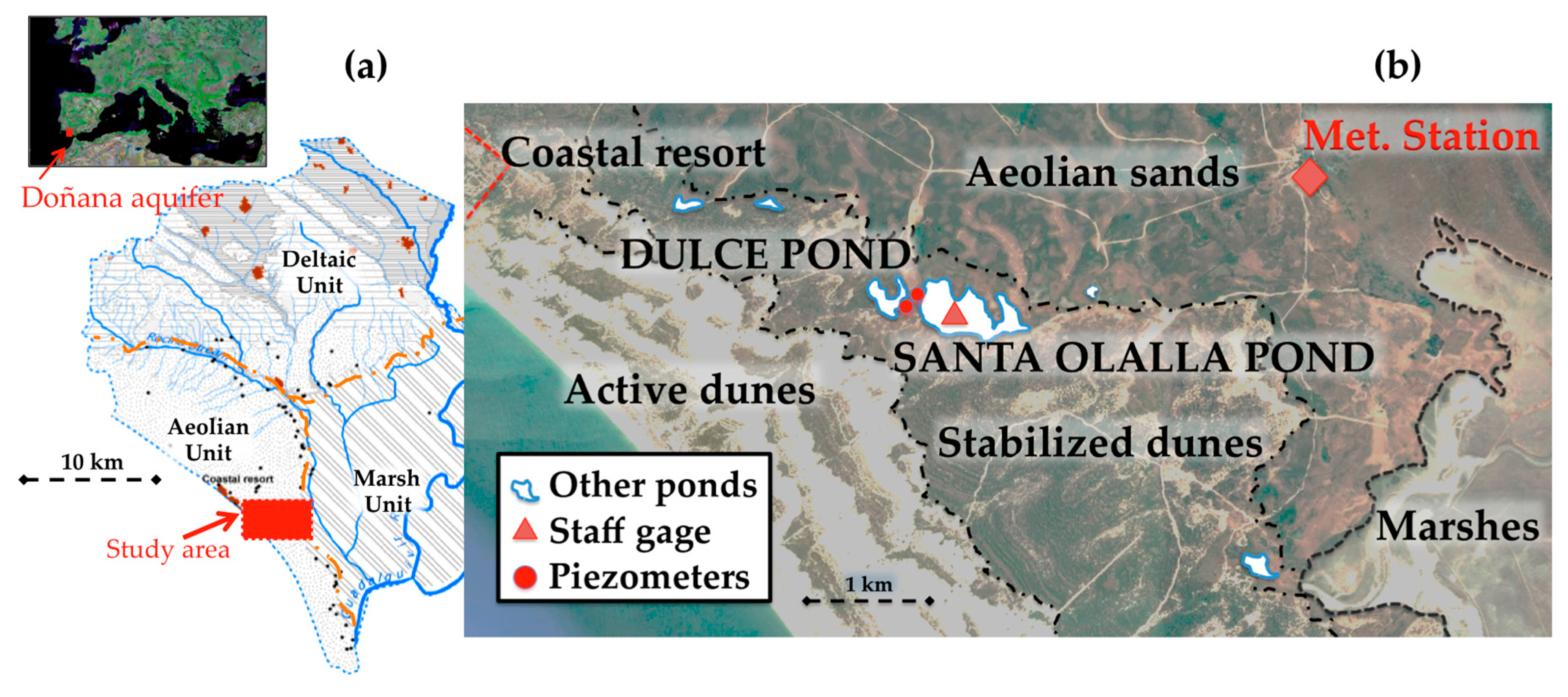
2. Materials and Methods
3. Results
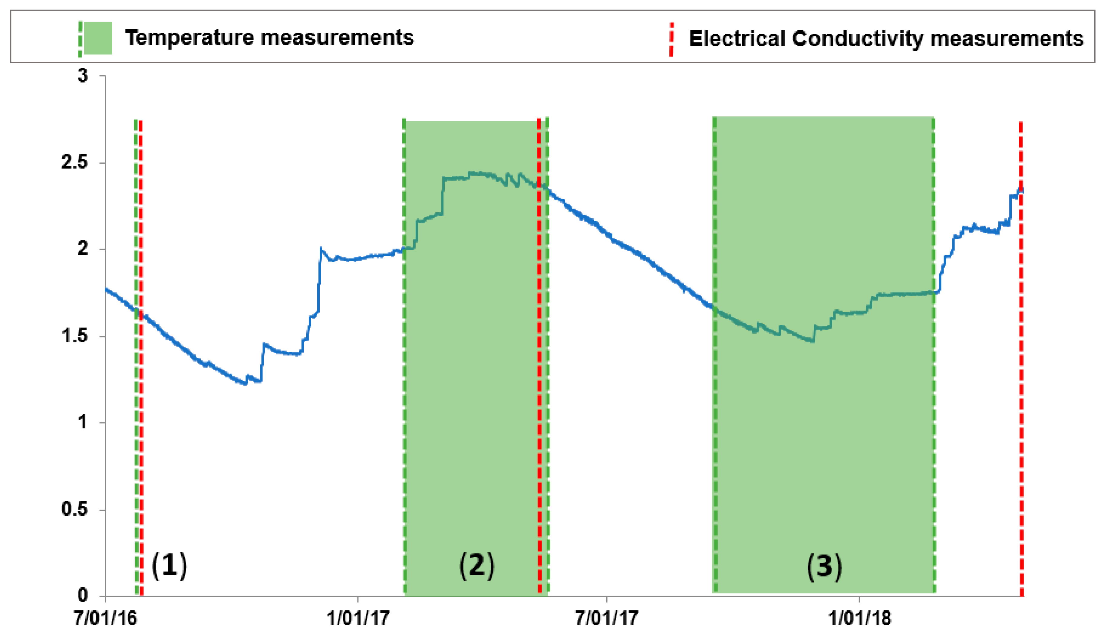
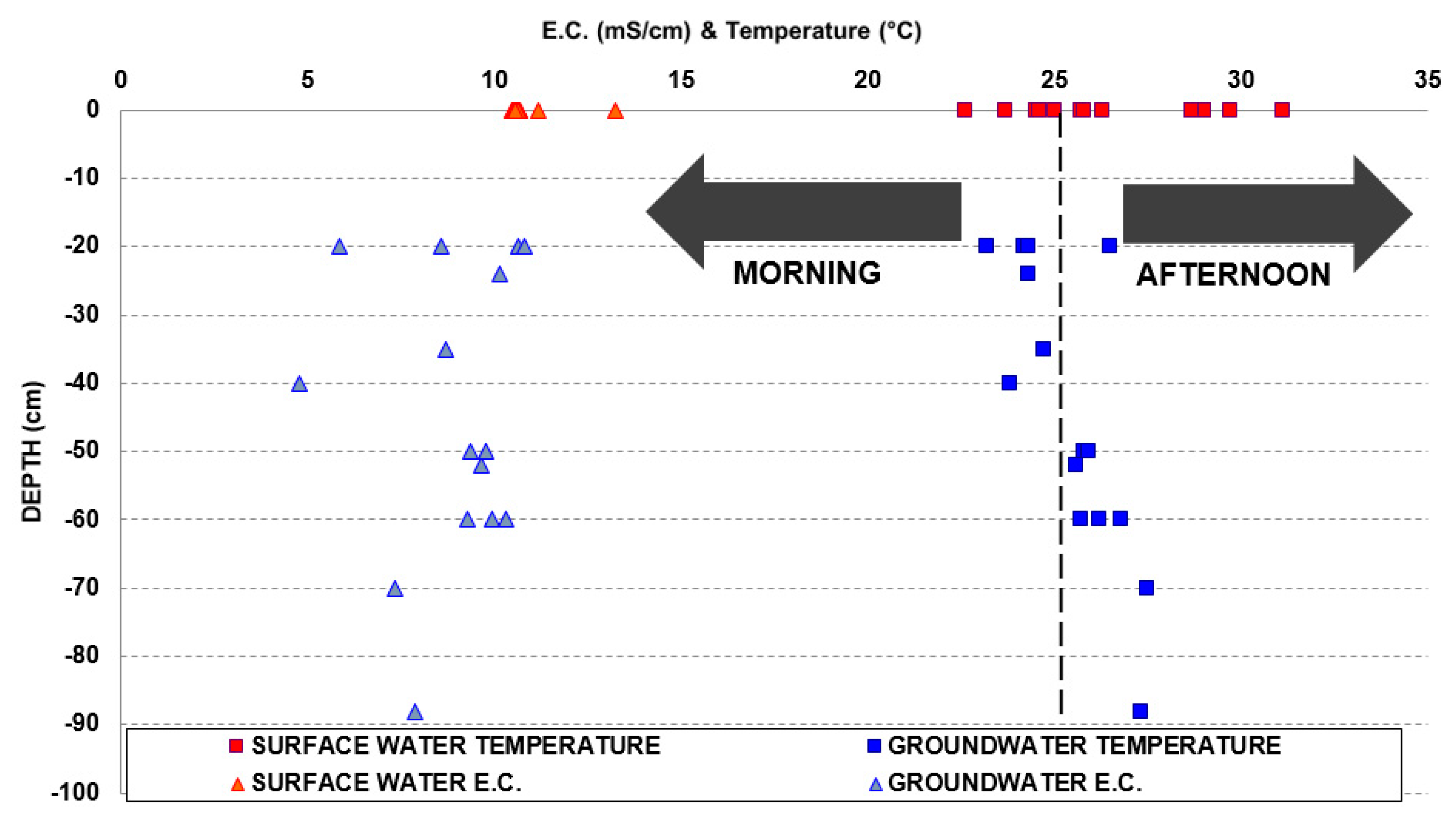
3.1. Field Campaigns in May–July (2016–2017–2018)
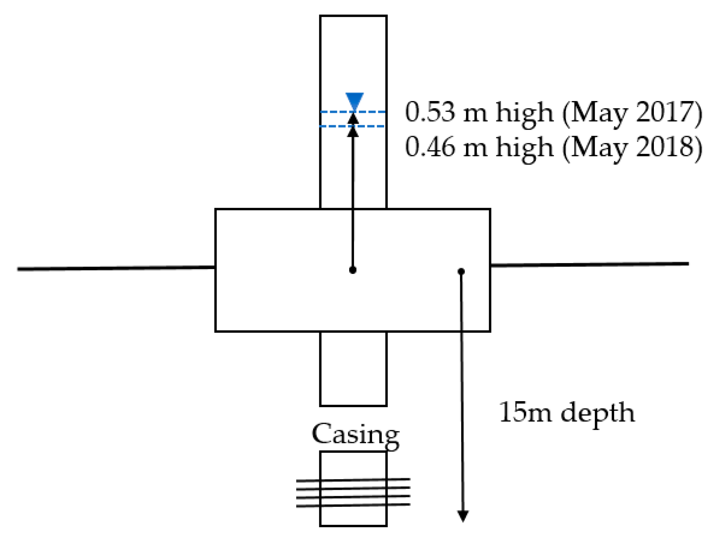
3.2. Heat Transfer Modelling to Estimate Groundwater Discharge
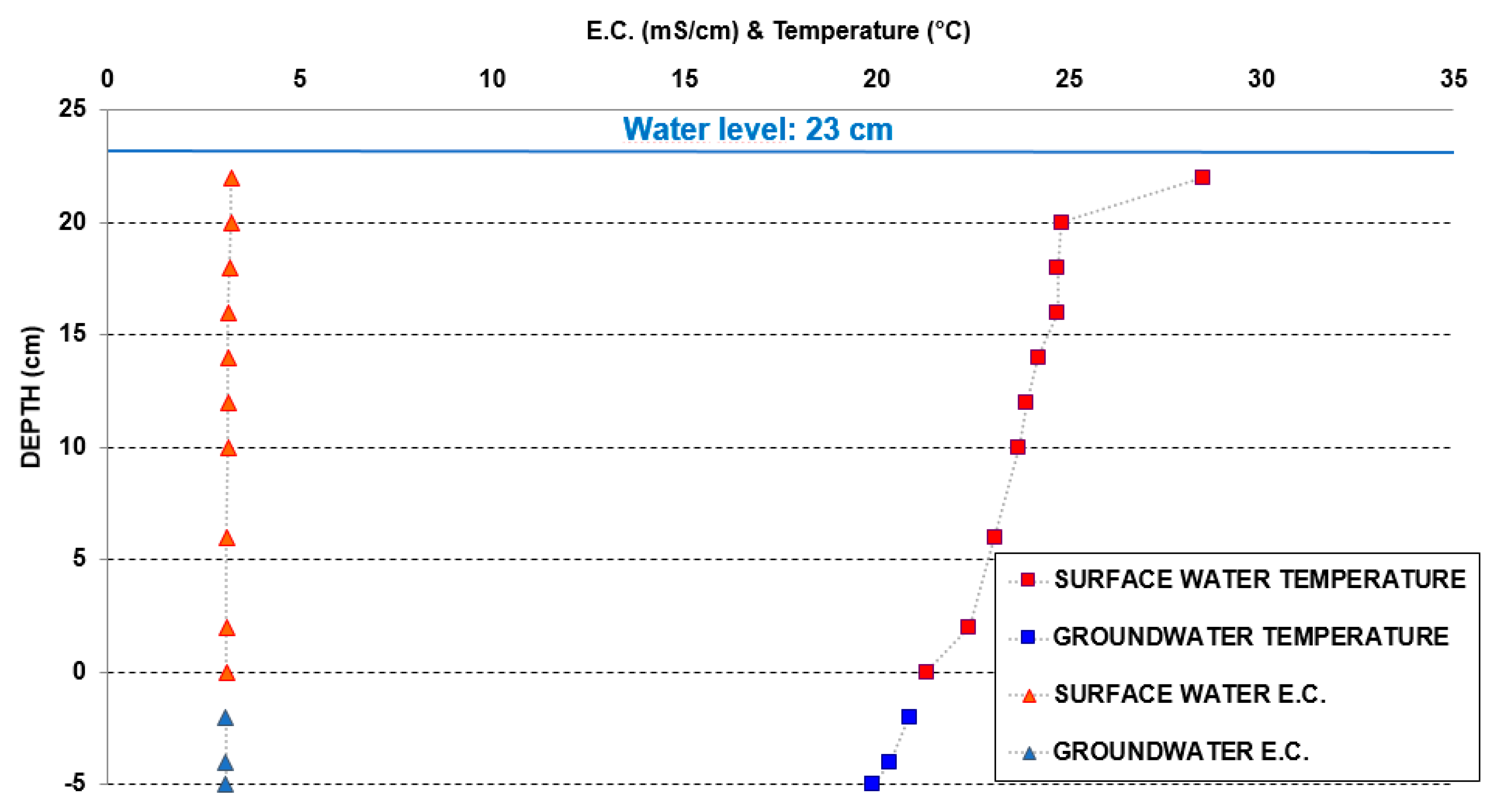
3.3. Thermal Behavior and Heat Transfer Modelling to Estimate Groundwater during Low Water Depth
4. Discussion
5. Conclusions
Author Contributions
Funding
Acknowledgments
Conflicts of Interest
Appendix A

| Location | Date | Time | EC (mS/cm) | Temperature (°C) | Depth (cm) |
|---|---|---|---|---|---|
| 1 | 12 July 2016 | 17:49 | 10.50 | 29.7 | 0 |
| 1 | 12 July 2016 | 05.84 | 26.5 | 20 | |
| 2 | 12 July 2016 | 18:07 | 10.47 | 29.0 | 0 |
| 2 | 12 July 2016 | 09.94 | 26.8 | 60 | |
| 3 | 12 July 2016 | 18:31 | 10.49 | 29.0 | 0 |
| 3 | 12 July 2016 | 10.32 | 25.7 | 60 | |
| 4 | 12 July 2016 | 18:50 | 10.50 | 28.7 | 0 |
| 4 | 12 July 2016 | 09.26 | 26.2 | 60 | |
| 5 | 12 July 2016 | 19:49 | 10.55 | 28.7 | 0 |
| 5 | 12 July 2016 | 07.35 | 27.5 | 70 | |
| 6 | 13 July 2016 | 10:20 | 10.63 | 22.6 | 0 |
| 6 | 13 July 2016 | 08.59 | 23.2 | 20 | |
| 7 | 13 July 2016 | 10:40 | 13.25 | 23.7 | 0 |
| 7 | 13 July 2016 | 04.77 | 23.8 | 40 | |
| 8 | 13 July 2016 | 10:58 | 10.68 | 24.5 | 0 |
| 8 | 13 July 2016 | 10.66 | 24.2 | 20 | |
| 9 | 13 July 2016 | 11:24 | 10.60 | 25.0 | 0 |
| 9 | 13 July 2016 | 08.68 | 24.7 | 35 | |
| 10 | 13 July 2016 | 11:51 | 10.61 | 24.6 | 0 |
| 10 | 13 July 2016 | 10.13 | 24.3 | 24 | |
| 11 | 13 July 2016 | 12:08 | 11.18 | 24.6 | 0 |
| 11 | 13 July 2016 | 10.82 | 24.3 | 20 | |
| 12 | 13 July 2016 | 12:48 | 10.70 | 25.7 | 0 |
| 12 | 13 July 2016 | 9.64 | 25.6 | 52 | |
| 13 | 13 July 2016 | 13:05 | 10.62 | 25.8 | 0 |
| 13 | 13 July 2016 | 09.35 | 25.8 | 50 | |
| 14 | 13 July 2016 | 13:27 | 10.65 | 26.3 | 0 |
| 14 | 13 July 2016 | 09.79 | 25.9 | 50 | |
| 15 | 13 July 2016 | 14:12 | 10.56 | 31.1 | 0 |
| 15 | 13 July 2016 | 07.89 | 27.3 | 88 |
Appendix B
| DISTANCE FROM SHORE (m) | EC (mS/cm) | pH | Temperature (°C) |
|---|---|---|---|
| SANTA OLALLA POND | |||
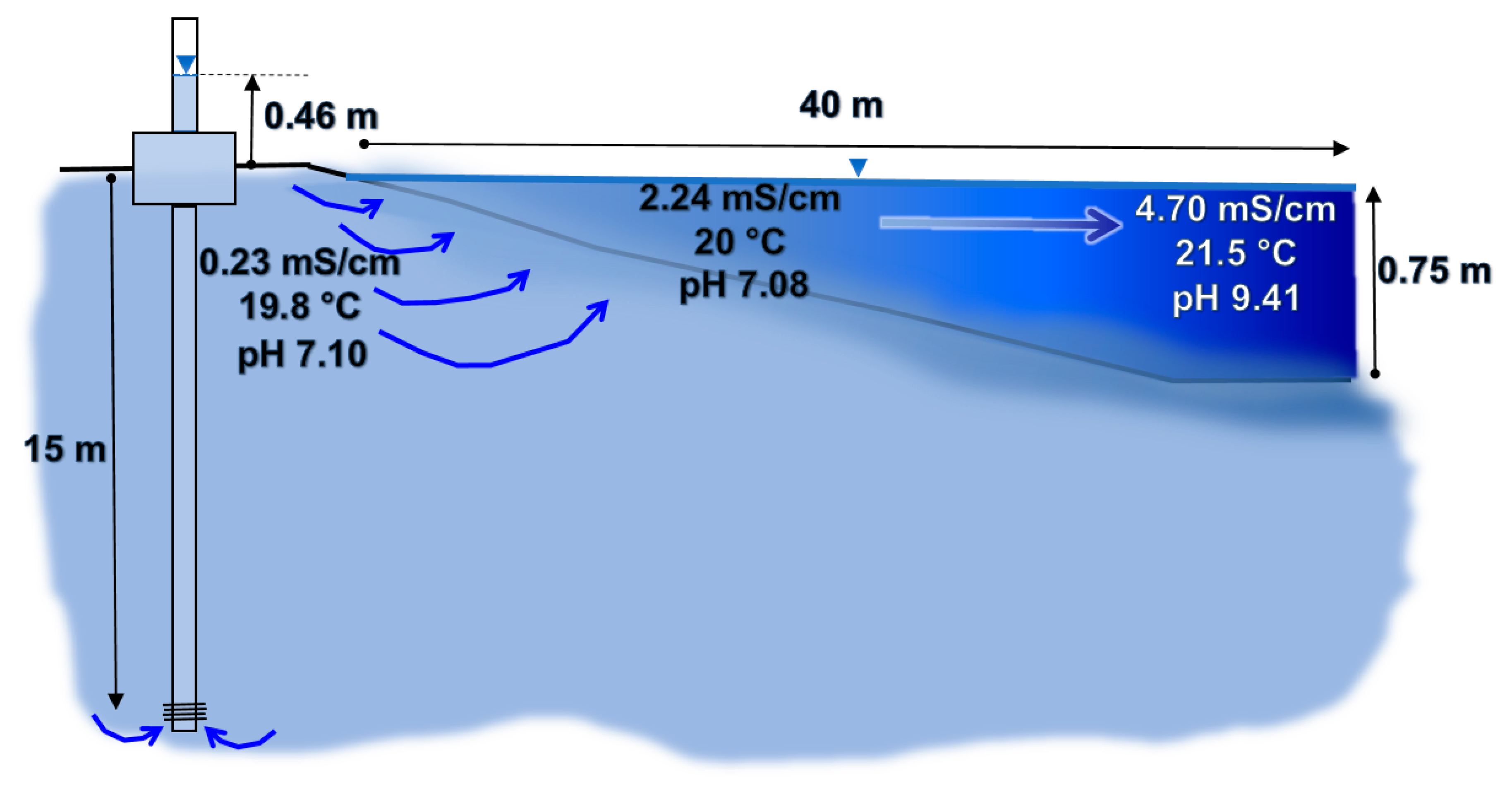
| 2 | 2.24 | 7.08 | 19.9 |
| 4 | 2.56 | 7.15 | 19.9 |
| 6 | 2.94 | 7.23 | 20.1 |
| 8 | 3.25 | 7.48 | 20.3 |
| 10 | 3.56 | 8.07 | 20.5 |
| 12 | 3.85 | 8.89 | 20.7 |
| 14 | 4.03 | 8.97 | 20.7 |
| 16 | 3.99 | 9.08 | 20.9 |
| 18 | 4.09 | 9.17 | 21.1 |
| 20 | 4.20 | 9.26 | 21.3 |
| 22 | 4.48 | 9.21 | 21.6 |
| 24 | 4.38 | 9.52 | 21.6 |
| 26 | 4.64 | 9.34 | 21.8 |
| 28 | 4.69 | 9.45 | 21.5 |
| 30 | 4.67 | 9.42 | 21.5 |
| 32 | 4.69 | 9.41 | 21.5 |
| 34 | 4.69 | 9.42 | 21.5 |
| 36 | 4.70 | 9.42 | 21.4 |
| 38 | 4.73 | 9.34 | 21.5 |
| 40 | 4.73 | 9.32 | 21.5 |
| DULCE POND | |||
| 2 | 1.22 | 7.11 | 20.0 |
| 4 | 1.22 | 7.23 | 20.1 |
| 6 | 1.19 | 7.09 | 19.9 |
| 8 | 1.15 | 7.15 | 20.3 |
| 10 | 1.11 | 7.31 | 20.7 |
| 12 | 1.10 | 8.06 | 21.2 |
| 14 | 1.10 | 8.22 | 21.4 |
| 16 | 1.10 | 8.41 | 21.6 |
| 18 | 1.10 | 8.53 | 21.9 |
| 20 | 1.10 | 8.54 | 21.8 |
| 22 | 1.10 | 8.58 | 21.8 |
References
- Green, A.J.; Alcorlo, P.; Peeters, E.T.; Morris, E.P.; Espinar, J.L.; Bravo-Utrera, M.A.; Bustamante, J.; Díaz-Delgado, R.; Koelmans, A.A.; Mateo, R.; et al. Creating a safe operating space for wetlands in a changing climate. Front. Ecol. Environ. 2017, 15, 99–107. [Google Scholar] [CrossRef] [Green Version]
- Lozano-Tomás, E. Las Aguas Subterráneas en Los Cotos de Doñana y su Influencia en Las Lagunas. Ph.D. Thesis, University Politécnica de Catalunya, Barcelona, Spain, 2004. [Google Scholar]
- Sacks, L.A.; Herman, J.S.; Konikow, L.F.; Vela, A.L. Seasonal dynamics of groundwater-lake interactions at Doñana National Park, Spain. J. Hydrol. 1992, 136, 123–154. [Google Scholar] [CrossRef]
- Swanson, T.E.; Cardenas, M.B. Ex-Stream: A MATLAB program for calculating fluid flux through sediment–water interfaces based on steady and transient temperature profiles. Comput. Geosci. 2011, 37, 1664–1669. [Google Scholar] [CrossRef]
- Bastola, H.; Peterson, E.W. Heat tracing to examine seasonal groundwater flow beneath a low-gradient stream in rural central Illinois, USA. Hydrogeol. J. 2016, 24, 181–194. [Google Scholar] [CrossRef]
- Irvine, D.J.; Lautz, L.K.; Briggs, M.A.; Gordon, R.P.; McKenzie, J.M. Experimental evaluation of the applicability of phase, amplitude, and combined methods to determine water flux and thermal diffusivity from temperature time series using VFLUX 2. J. Hydrol. 2015, 531, 728–737. [Google Scholar] [CrossRef] [Green Version]
- McCallum, A.M.; Andersen, M.S.; Rau, G.C.; Acworth, R.I. A 1-D analytical method for estimating surface water–groundwater interactions and effective thermal diffusivity using temperature time series. Water Resour. Res. 2012, 48. [Google Scholar] [CrossRef]
- Stonestrom, D.A.; Constantz, J. Heat as a Tool for Studying the Movement of Ground Water Near Streams; U.S. Department of the Interior, U.S. Geological Survey: Reston, WV, USA, 2003; Volume 1260.
- Rodríguez-Rodríguez, M.; Martos-Rosillo, S.; Fernández-Ayuso, A.; Aguilar, R. Application of a flux model and segmented-Darcy approach to estimate the groundwater discharge to a shallow pond. Case of Santa Olalla pond. Geogaceta 2018, 63, 27–30. [Google Scholar]
- Fernández-Ayuso, A.; Rodríguez-Rodríguez, M. Estimation of hydrogeological parameters by tidal influence methods in the recharge area of the sand aquifer in Doñana National Park (Huelva, Spain). Geogaceta 2018, 64. in press. [Google Scholar]
- Koch, F.W.; Voytek, E.B.; Day-Lewis, F.D.; Healy, R.; Briggs, M.A.; Werkema, D.; Lane, J.W., Jr. 1DTempPro: A program for analysis of vertical one-dimensional (1D) temperature profiles v2.0. U.S. Geol. Surv. Softw. Release 2015. [Google Scholar] [CrossRef]
- Goto, S.; Matsubayashi, O. Inversion of needle probe data for sediment thermal properties in the eastern flank of the Juan de Fuca Ridge. J. Geophys. Res. 2008, 113. [Google Scholar] [CrossRef]
- Silliman, S.E.; Booth, D.F. Analysis of time-series measurements of sediment temperature for identification of gaining vs. losing portions of Juday Creek, Indiana. J. Hydrol. 1993, 146, 131–148. [Google Scholar] [CrossRef]
- Jensen, K.H.; Bitsch, K.; Bjerg, P.L. Large-scale dispersion experiments in a sandy aquifer in Denmark: Observed tracer movements and numerical analyses. Water Resour. Res. 1993, 29, 673–696. [Google Scholar] [CrossRef]
- Rosenberry, D.O.; Hayashi, M. Assessing and measuring wetland hydrology. In Wetland Techniques; Anderson, T., Davis, C.A., Eds.; Springer: Dordrecht, The Netherlands, 2013; Volume 1, pp. 87–225. ISBN 978-94-007-6860-4. [Google Scholar]


| Modeling Conditions 1D Temp PRO V.2 | |
|---|---|
| Porosity | 0.3 (m3/m3) 1 |
| Thermal conductivity | 1 (W/m°C) 2 |
| Sediment heat capacity | 3.3 × 10⁶ (J/m3°C) 2 |
| Dispersivity | 5 × 10⁻⁴ m 3 |
© 2018 by the authors. Licensee MDPI, Basel, Switzerland. This article is an open access article distributed under the terms and conditions of the Creative Commons Attribution (CC BY) license (http://creativecommons.org/licenses/by/4.0/).
Share and Cite
Rodríguez-Rodríguez, M.; Fernández-Ayuso, A.; Hayashi, M.; Moral-Martos, F. Using Water Temperature, Electrical Conductivity, and pH to Characterize Surface–Groundwater Relations in a Shallow Ponds System (Doñana National Park, SW Spain). Water 2018, 10, 1406. https://doi.org/10.3390/w10101406
Rodríguez-Rodríguez M, Fernández-Ayuso A, Hayashi M, Moral-Martos F. Using Water Temperature, Electrical Conductivity, and pH to Characterize Surface–Groundwater Relations in a Shallow Ponds System (Doñana National Park, SW Spain). Water. 2018; 10(10):1406. https://doi.org/10.3390/w10101406
Chicago/Turabian StyleRodríguez-Rodríguez, Miguel, Ana Fernández-Ayuso, Masaki Hayashi, and Francisco Moral-Martos. 2018. "Using Water Temperature, Electrical Conductivity, and pH to Characterize Surface–Groundwater Relations in a Shallow Ponds System (Doñana National Park, SW Spain)" Water 10, no. 10: 1406. https://doi.org/10.3390/w10101406