Computationally Efficient Multivariate Calibration and Validation of a Grid-Based Hydrologic Model in Sparsely Gauged West African River Basins


1
Department of Geography, University of Bonn, Meckenheimer Allee 166, 53115 Bonn, Germany
2
UFZ—Helmholtz Centre for Environmental Research, 04318 Leipzig, Germany
*
Author to whom correspondence should be addressed.
Water 2018, 10(10), 1418; https://doi.org/10.3390/w10101418
Submission received: 6 September 2018
/
Revised: 2 October 2018
/
Accepted: 8 October 2018
/
Published: 10 October 2018
(This article belongs to the Special Issue Enhancing Hydrological Prediction through Modelling with Large Datasets)
Abstract
:The prediction of freshwater resources remains a challenging task in West Africa, where the decline of in situ measurements has a detrimental effect on the quality of estimates. In this study, we establish a series of modeling routines for the grid-based mesoscale Hydrologic Model (mHM) using Multiscale Parameter Regionalization (MPR). We provide a computationally efficient application of mHM-MPR across a diverse range of data-scarce basins using in situ observations, remote sensing, and reanalysis inputs. Model performance was first screened for four precipitation datasets and three evapotranspiration calculation methods. Subsequently, we developed a modeling framework in which the pre-screened model is first calibrated using discharge as the observed variable (mHM Q), and next calibrated using a combination of discharge and actual evapotranspiration data (mHM Q/ET). Both model setups were validated in a multi-variable evaluation framework using discharge, actual evapotranspiration, soil moisture and total water storage data. The model performed reasonably well, with mean discharge KGE values of 0.53 (mHM Q) and 0.49 (mHM Q/ET) for the calibration; and 0.23 (mHM Q) and 0.13 (mHM Q/ET) for the validation. Other tested variables were also within a good predictive range. This further confirmed the robustness and well-represented spatial distribution of the hydrologic predictions. Using MPR, the calibrated model can then be scaled to produce outputs at much smaller resolutions. Overall, our analysis highlights the worth of utilizing additional hydrologic variables (together with discharge) for the reliable application of a distributed hydrologic model in sparsely gauged West African river basins.
1. Introduction
Due to economic conditions in many West African countries, between 50 and 60% of the labor force works in the agricultural sector, mostly as self-sustaining farmers generating income by selling surpluses and cash-crops not intended for local consumption [1,2,3]. Therefore, water availability not only directly influences the food security of large parts of the population, but also economic development [4]. The estimation of available water resources using hydrologic modeling provides important information for planners and policy makers to mitigate problems arising due to water shortages. The subject of performing hydrologic predictions in sparsely gauged West African river basins has been well covered in recent years [4,5,6,7,8,9,10,11]. Due to a continuous decline in ground-based observation networks as a consequence of political unrest and financial instability [12,13], the authors explored the possibility of setting up the semi-distributed Soil and Water Assessment Tool (SWAT) model [14,15,16] for several West African river basins in a previous study [11]. While multi-objective validation of streamflow, actual evapotranspiration, soil moisture dynamics, and total water storage revealed the model to provide robust results, the applied scale was coarse due to computational constrains, with the smallest areas of fully distributed estimations, called subbasins in SWAT, being at least 500 km2 large.
Hydrologic models are generally calibrated by optimizing multiple free parameters to fit a model output against an observation using objective functions to measure the performance of the solution [17]. The continuous increase in computational power and availability of remotely sensed data for model parametrization has given rise to complex spatially distributed and semi-distributed hydrologic models in recent years [18]. Well-known examples for this are the spatially distributed MIKE-SHE model [19], and the semi-distributed SWAT model [14,15,16]. However, especially at the mesoscale, the main problems of contemporary hydrology—nonlinearity, scale, uniqueness, equifinality and uncertainty—remain [20]. It has been suggested that these problems are not adequately addressed by the continuous increase in model complexity, which does not necessarily relate to an improved performance. Especially, overparameterization and subsequent parameter equifinality are cited as key problems [18,21,22]. In spatially distributed models, free parameters have to be inferred through calibration for each modeling unit, thus increasing the number of parameters if the model resolution is increased [23,24]. One technique for reducing the number of free parameters is the Hydrological Response Unit (HRU) approach, applied, among others, by SWAT, where modeling units of the same physical characteristics (soil, land use, slope, etc.) are first grouped and then calibrated together [14,25,26]. Another method of parameter reduction, which is applied by the mesoscale Hydrologic Model (mHM) [18,21], is multiscale parameter regionalization (MPR) [18]. In MPR, model parameters and physical basin parameters are connected via a priori defined relationships, e.g., through pedotransfer functions, and only the global parameters that define these relationships are optimized by calibration [18,21].
Multiple studies have explored the performance of the mHM model, mostly for the European continent [18,21,26,27,28,29,30,31,32]. Kauffeldt et al. [33] give an overview of 24 large-scale hydrologic models and their suitability for the European Flood Awareness System. They state that mHM fulfills almost all requirements and needs little modification to be adopted. More recently, mHM has also been included in the Inter-Sectoral Impact Model Intercomparison Project—regional water sector (ISI-MIP; www.isimip.org), which analyzes forcing and model uncertainties using an ensemble of hydrologic models and climate scenarios for multiple regions on a century-long timescale, including the Blue Nile and Niger river basins [34,35,36,37].
It has been shown by Rakovec at al. [29] that the implementation of Gravity Recovery and Climate Experiment (GRACE)-derived total water storage data significantly improves the partitioning of rainfall into the runoff components without impairing discharge simulations in 83 European river basins. Furthermore, mHM was used in the framework of the German drought monitor, where a drought map for the whole of Germany was generated using mHM soil moisture estimations [38]. mHM has also been used to produce a high-resolution dataset of water fluxes for Germany by running the model for seven large German river basins and validating the results using 222 additional streamflow stations, as well as evapotranspiration, soil moisture and groundwater recharge data. Results have shown the model to capture the daily streamflow dynamics at the calibrated stations very well and to also sufficiently estimate stations not included in the calibration. Daily actual evapotranspiration evaluated against multiple eddy covariance stations showed little bias and no systematic over- or underestimation. Soil moisture anomalies also proved to be in good agreement with the observations. Spatial patterns of actual evapotranspiration and groundwater recharge evaluated against the observations again showed good agreement [30]. The application of the model in a data-scarce basin in India using remote sensing data for model parametrization also produced promising results [39].
While calibrating and validating a hydrologic model using discharge observations allows the modeler to confidently predict runoff, the same cannot be said for the representation of other hydrologic processes due to parameter equifinality [11,28]. If, e.g., modeled discharge is to be reduced to fit observations during calibration, the same effect can be achieved by increasing either actual evapotranspiration or percolation. Since the prediction of spatially distributed hydrologic components such as evapotranspiration, soil moisture or total water storage is increasingly desired, multivariate calibration and validation is of immense value in producing realistic results other than streamflow [28,29,40]. This holds especially true for data-scarce regions.
Earlier studies have shown the scaling capabilities of mHM-MPR in Europe and the United States [27,28]. This approach will be tested in the data-scarce West African domain for the first time. In this study, we assess the scalability of mHM as argued by Kumar et al. [27] by calibrating the model at a computationally efficient coarse scale and running the calibrated model in finer resolutions. If the scaling capability of the model has been proven to perform well, it can then be used to generate hydrologic outputs at much smaller, local scales for various research and policy applications. Furthermore, this approach could be utilized to include other hydrologic variables at their native resolutions without introducing bias through data aggregation and disaggregation [28].
The objectives for this study are therefore (1) to investigate the performance of the mHM model using a multiscale parameter regionalization approach for selected sparsely gauged West African river basins under different precipitation inputs, (2) to assess the multivariate calibration options of mHM by calibrating the model for streamflow and actual evapotranspiration and validating against these, as well as against soil moisture and total water storage anomaly datasets, and (3) to assess the transferability of model parameters inferred through MPR between different spatial resolutions.
This study is part of the German Research Foundation-funded COAST (studying changes of sea level and water storage for coastal regions in West Africa using satellite and terrestrial data sets) project. The work builds on previously published studies [11,41], with the main focus being the assessment of the contribution of remote sensing evapotranspiration, soil moisture and total water storage estimates in hydrologic simulations of data-scarce basins.
2. Materials and Methods
2.1. Study Area
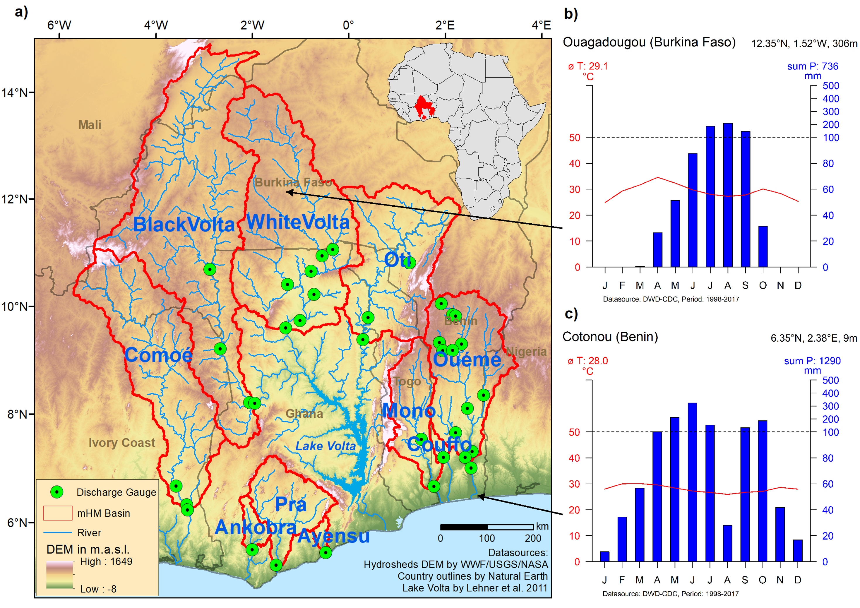
The study area in southern West Africa, located between 4.5 and 15° latitude and −6 and 3.5° longitude, is presented in Figure 1a. The topography of the study area is flat, with the highest mountain range stretching from southern Ghana (Akwapim Hills) through Togo (Togo Mountains) and into northern Benin (Atakora Mountains) [42]. The highest peaks reach almost 1000 m according to DEM data [43,44]. Rainfalls in the region are strongly seasonal; bimodal in the south (e.g., Cotonou, see Figure 1b) and unimodal in the north (e.g., Ouagadougou, see Figure 1c), with a distinct south-north gradient of reducing rainfall sums [45,46,47]. Ten river basins were chosen to be modeled based on the availability of streamflow records for calibration and validation: Comoé (Ivory Coast, Ghana and Burkina Faso, 74,604 km2, three gauges), Ouémé (Benin, Nigeria and Togo, 47,562 km2, 13 gauges), Couffo (Benin and Togo, 1672 km2, one gauge), Mono (Togo and Benin, 22,711 km2, two gauges), Pra (Ghana, 22,733 km2, one gauge), Ayensu (Ghana, 1699 km2, one gauge), Ankobra (Ghana, 4246 km2, one gauge), Black Volta (Burkina Faso, Ivory Coast, Ghana and Mali, 138,440 km2, four gauges), White Volta (Burkina Faso, Ghana and Togo, 100,036 km2, seven gauges), and Oti (Burkina Faso, Togo, Benin and Ghana, 60,015 km2, three gauges). Basin areas are relative to the last modeled gauging station and not the entire river basin. In total, 473,718 km2 and 36 streamflow gauging stations were modeled.
2.2. The Mesoscale Hydrologic Model (mHM)
The mesoscale Hydrologic Model (mHM) [18,21] is a spatially explicit, grid-based hydrologic model created specifically for providing distributed predictions of hydrologic variables like runoff, evapotranspiration, soil moisture and discharge along the river network. The main components of mHM are based on well-established hydrologic process descriptions of large-scale models like HBV [48,49] and VIC [50]. mHM accounts for the following processes: canopy interception, snow accumulation and melting, soil moisture dynamics, infiltration, surface runoff, discharge generation, evapotranspiration, subsurface storage, deep percolation, baseflow, and flood routing [18].
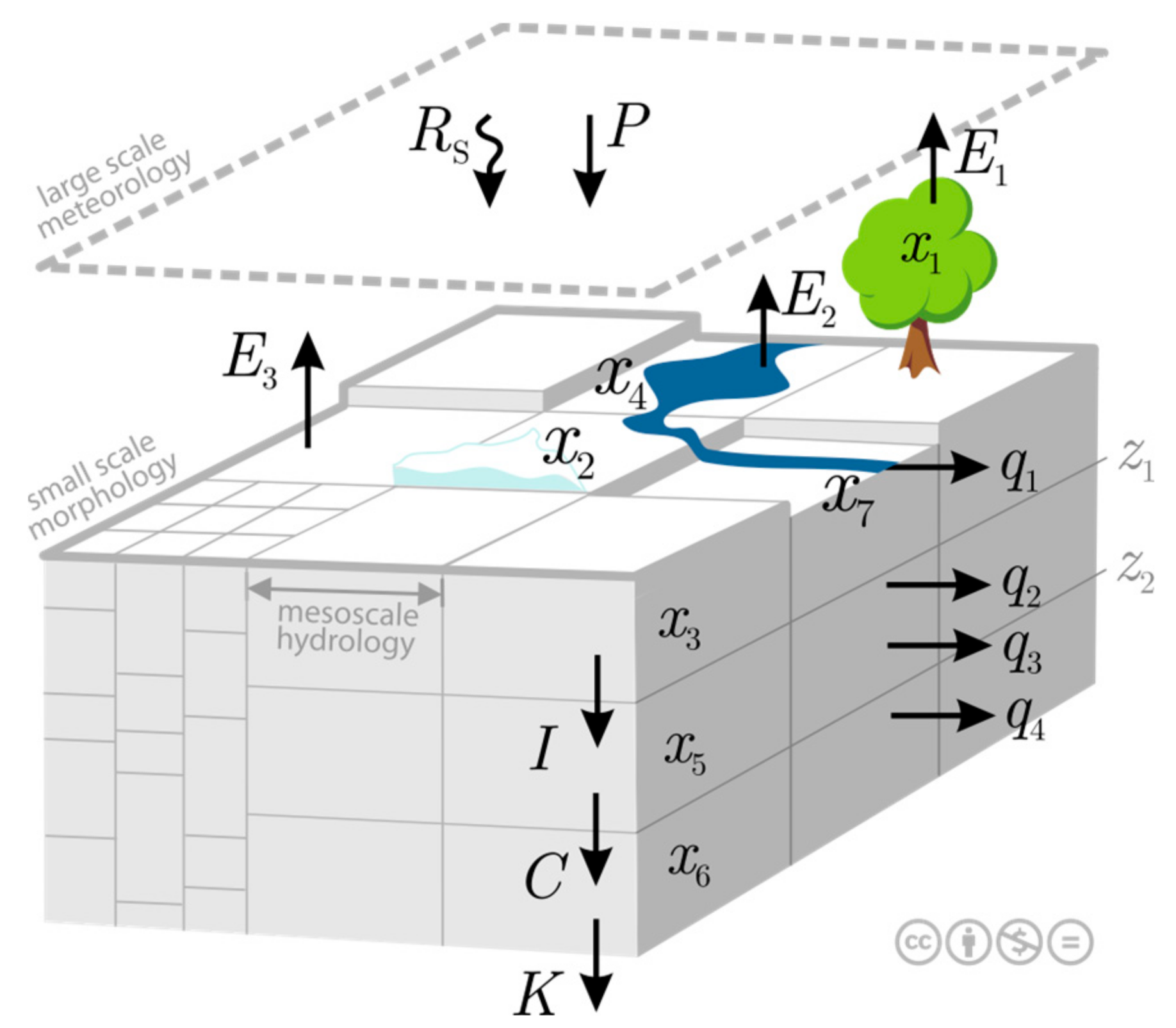
In mHM, different (spatial) levels of modeling components are considered to better account for the spatial variability of inputs and hydrologic processes. A schematic overview of mHM is given in Figure 2. The model source code is freely available, and further details can be found at www.ufz.de/mhm. The finest-resolution category is the small-scale morphological input class Level 0 (L0). This class contains variables such as elevation, slope, soil, and land use. The next highest resolution, Level 1 (L1) represents the resolution of the hydrologic model routines and output and only requires the regionalized fields of model parameters (see below). Level 2 (L2) is the coarsest-resolution category, containing the large-scale meteorological forcing inputs such as precipitation and temperature [18,51]. mHM uses a novel Multiscale Parameter Regionalization (MPR) approach to estimate the regionalized fields of model parameters first at the L0 resolution. Then, an upscaling operator is used to generate effective parameters at the L1 modeling resolution. Regionalization at the L0 scale is performed by linking the model parameters to available catchment attributes (terrain, slope and aspect, soil textural and land cover properties) via a set of pedotransfer functions and free calibration parameters (see [18,21] for further details). The MPR approach significantly reduces the number of free (calibration) parameters while accounting for the spatial variability of model parameters required for distributed hydrologic model applications (see [52] for details on estimation of key soil hydrologic parameters using MPR). Kumar et al. [21] found both MPR and HRU approaches to perform similarly regarding daily streamflow predictions in 45 calibrated southern German river basins. However, MPR proved to be superior in the preservation of spatiotemporal patterns of water fluxes and, since free parameters of MPR are not scale-specific, they can be transferred to different modeling scales without time-intensive recalibration and without introducing significant bias. This effectively means that mHM can be calibrated at a computationally efficient, coarser L1 resolution and that the calibrated (free) parameters can then be transferred to a finer resolution. Further studies also demonstrated the scaling capabilities of mHM on comparatively large domains of European basins and the Mississippi river basin [27,28].
mHM offers multiple optimization algorithms, such as Monte Carlo Markov Chain (MCMC), Dynamically Dimensioned Search (DDS), Simulated Annealing (SA) and Shuffled Complex Evolution (SCE) [51]. In this study, the Dynamically Dimensioned Search algorithm was used. DDS has been shown to perform well when compared to SCE, converging on a good solution in only 15 to 20% of the model runs required by SCE while also avoiding local optima [53]. Behrangi et al. [54] noted that DDS finds a solution faster than SCE because it has been developed especially for computationally demanding models, while SCE was originally developed for lumped models, and go on to show that SCE may be adapted to decrease the number of iterations needed to find a good solution. The authors suggest a large number of model iterations to ensure good solutions are found by DDS.
2.3. Input Data
2.3.1. Morphological Inputs
The HydroSHEDS (Hydrological data and maps based on SHuttle Elevation Derivatives at multiple Scales) hydrologically conditioned digital elevation model (DEM) [43,44] was used as a basis to create the morphological input data. The DEM is based on Shuttle Radar Topographic Mission (SRTM) data and was developed by the World Wildlife Fund (WWF) and the United States Geological Survey (USGS). While available in multiple resolutions, in this study the 500 m resolution was used. The required slope, aspect, flow direction and flow accumulation data were derived from this dataset.
2.3.2. Soil Inputs
Concerning soil input data, a raster dataset with the location of soil classes and a corresponding lookup table with the attributes’ depth, texture and bulk density are required. This information was compiled from the Harmonized World Soil Database (HWSD) version 1.2 [55]. The dataset contains physical and chemical parameters for a topsoil (0–30 cm) and subsoil (>30–100 cm) layer at a 1 km resolution.
2.3.3. Land Use Inputs
Two land use inputs are necessary, a Land Use and Land Cover (LULC) map and a Leaf Area Index (LAI) class map with a corresponding lookup table. While mHM recognizes only three LULC classes (forest, pervious, impervious), an arbitrary number of LAI classes can be defined. Both maps were generated using the Globcover 2.3 product developed by the European Space Agency (ESA), representing the global land cover of the year 2009, available at a 300 m resolution [56]. To generate the mHM LULC map, Globcover classes were reclassified to the three mHM classes. The mHM LAI class map was produced using the original Globcover classes and calculating long-term monthly LAI values (2003–2013) for each class from MODerate-resolution Imaging Spectroradiometer (MODIS) MCD15A2v5 LAI data, produced by the National Aeronautics and Space Administration (NASA) [57,58].
2.3.4. Meteorological Inputs
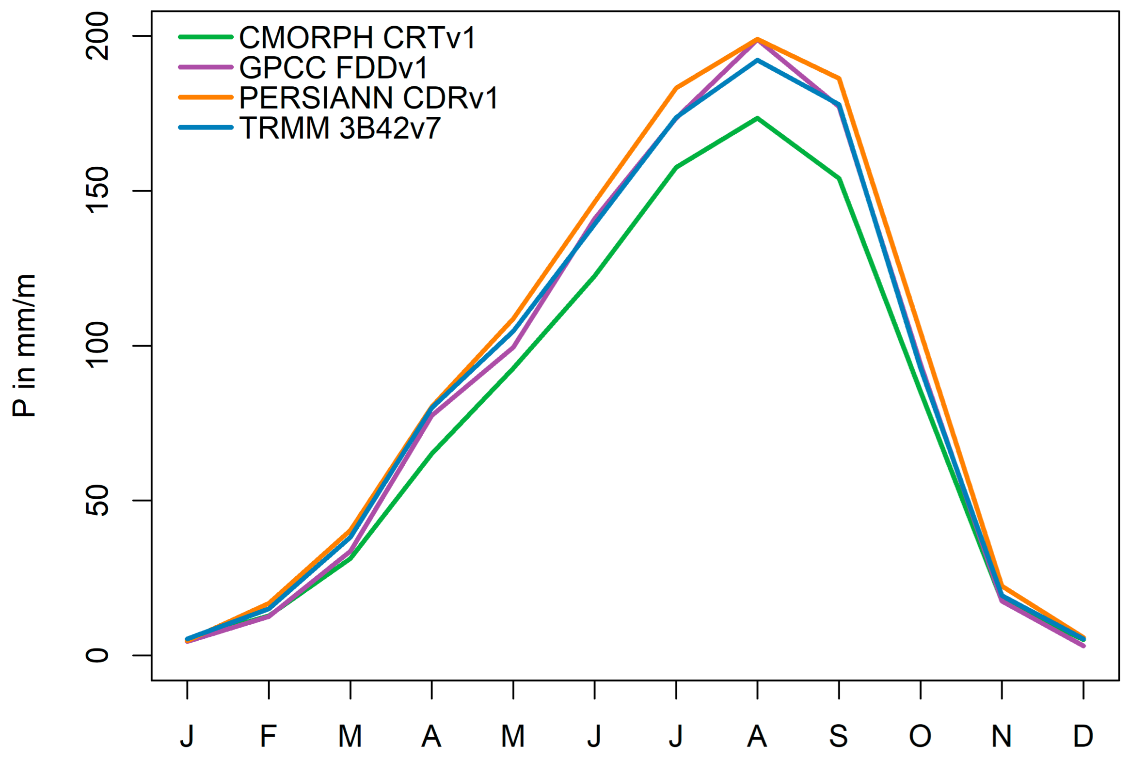
In Poméon et al. [41], ten remotely sensed and reanalyzed precipitation datasets were evaluated for the study region. Products relying on a combination of satellite microwave and infrared measurements as well as bias correction using ground-based data generally performed best. Four of the best-performing datasets were chosen for exploratory mHM runs. The combination that performed best in the exploratory runs was used for model calibration. Firstly, the Climate Prediction Center Morphing Technique (CMORPH) v1 CRT was chosen, which is globally available at a 0.25° resolution from 1998 onwards [59,60]. CMORPHv1 CRT, hereafter named CMORPH, was also used in SWAT simulations of sparsely gauged river basins in West Africa [11]. Secondly, the Tropical Rainfall Measuring Mission—Multi-satellite Precipitation Analysis (TRMM-MPA) product version 3B42v7, hereafter named TMPA, was evaluated. It is available from 50° north to 50° south at a 0.25° resolution from 1998 onwards [61]. Further evaluated was PERSIANN CDR version 1, available from 60° north to 60° south at a 0.25° resolution [62]. All three products include bias-corrected satellite microwave and infrared measurements [59,60,61,62]. Lastly, the Global Precipitation Climatology Centre Full Data Daily (GPCC FDD) version 1 global rain gauge product, developed by the German Meteorological Agency at a 1° resolution, was evaluated [63]. For more information on the used precipitation datasets, please refer to [41]. While rainfall dynamics are very similar for all datasets, CMORPH estimates on average slightly less precipitation during the peak of the wet season from June to September (Figure 3). For the 1998 to 2013 long-term monthly average, CMORPH predicts 77 mm monthly precipitation, TRMM 87 mm, PERSIANN 92 mm and GPCC 86 mm.
Depending on the method chosen to model the potential evapotranspiration (ETP), further meteorological inputs are needed to run mHM [51]. Three methods were evaluated in this study, namely: the estimation based on air temperature data using the Hargreaves-Samani method [64] and a direct in-built read-in of potential evapotranspiration estimates with either LAI or aspect correction. Minimum and maximum 2 m daily temperature was extracted from NASA Modern-Era Retrospective analysis for Research and Applications 2 (MERRA 2) reanalysis data, available at a global grid of 0.625° × 0.5° from 1980 onwards [65]. Potential evapotranspiration data was obtained from the Global Land Evaporation Amsterdam Model (GLEAM) v3.1a [66,67]. GLEAM data was chosen since it is availible for the studied period (model warm-up starting in 1998) at a daily timestep.
2.3.5. Discharge Inputs
The discharge data used for calibrating and validating the mHM model was obtained from the German Global Runoff Data Center (GRDC), the French AMMA-CATCH (Analyse Multidisciplinaire de la Mousson Africaine-Couplage de l’Atmosphère Tropicale et du Cycle Hydrologique) regional observing system, and through personal communication with local agencies and partners. Due to different observation periods and gaps in the discharge data that did not allow for fixed calibration and validation periods, two thirds of the data were used for calibration and one third for validation [11,68].
2.3.6. Validation Data
Multivariate validation of the modeled soil moisture, actual evapotranspiration and total water storage anomalies was furthermore performed. For the soil moisture validation, the ESA Climate Change Initiative (CCI) soil moisture (v4.2; www.esa-soilmoisture-cci.org) combined product was used. The combined product was created by merging active scatterometer and passive soil moisture retrievals from multiple satellites. Daily retrievals, although only in the satellite swaths, are available at a resolution of 0.25° [69,70,71,72,73]. Three different datasets were used for the validation of the actual evapotranspiration, namely MODIS MOD16A2 [74,75], GLEAM 3.2a and GLEAM 3.2b [66,67]. MOD16A2 ETP estimates were further used to validate model results during the exploratory model runs. For the validation of total water storage anomaly (ΔTWS), remotely sensed GRACE retrievals from ITSG-Grace 2016 time series provided by the Institute of Geodesy at Technical University Graz [76] and adapted for the study area [11] were used. GRACE estimates are available at a minimum spatial resolution of 400 × 400 km and a temporal resolution of 30 days [77]. While the model can be calibrated using TWS, the processed timeseries covers all basins and cannot be further spatially disaggregated into single basins.
2.4 Framework of the Modeling Experiment
To be able to place confidence in the model output, the following framework was developed, where the input data and modeling routines are examined in twelve default simulation runs before the model is optimized. In the first step after preparing the input data and setting up the model, a simulation using the default parameter values was performed. For each subsequent run, the precipitation inputs were varied between the four datasets (CMORPH, GPCC, PERSIANN and TMPA). Likewise, the potential evapotranspiration calculation method was changed between three options available in mHM, namely the Hargreaves-Samani temperature-based method (HAR), read-in with automatic LAI correction (LAI) and read-in with automatic aspect-driven correction (ASP) [51] for each precipitation dataset. A graphical overview of the setup and associated combination numbers is presented in Figure 4. In our case, the model is run at a daily timestep from 1998 to 2013, with the year 1998 considered as the warm-up period. While daily streamflow outputs are produced, other variables are output at a monthly resolution for better comparison to monthly remote sensing estimates.
It has been shown that precipitation estimates have a strong impact on model performance [41,78]. The performance of the simulated streamflow, potential and actual evapotranspiration and total water storage anomaly were evaluated for each combination. Once the best initial combination was determined, the most efficient model resolution was chosen by running the previously defined simulation at different resolutions and evaluating the required runtime for each resolution. After establishing the best combination of precipitation input data, evapotranspiration calculation method, and modeling resolution, the model was calibrated for each river basin separately using discharge records as the observed variable. The optimization method based on the Kling-Gupta Efficiency (KGE) measure was chosen in this study. KGE offers the advantage of including correlation, bias and relative variability in its composition. The dimensionless result ranges from −∞ to 1 [79] and will be regarded as acceptable from 0.5 upwards. For the chosen optimization method, mHM calculates 1 minus the average KGE, where all stations within the specific basin are weighted equally.
As a separate setup, the model was calibrated using an optimization method which includes both discharge and basin-wide mean actual evapotranspiration (where we used GLEAM 3.2a), as shown in Equation (1).
where is the mHM objective function 30, is the average Kling-Gupta Efficiency of the discharge simulation (all stations are again weighted equally) and is the root mean squared error of the basin average actual evapotranspiration (ETA) simulation.
The second calibration was chosen to assess the gains of calibrating the model using an additional dataset (complimenting discharge observations). This approach can be especially useful in sparsely gauged regions, such as West Africa, where only few discharge observations exist, but remote sensing evapotranspiration estimates are easily available. Also, more realistic model results may be obtained if using multiple observed variables in the calibration [29]. mHM may also be calibrated using SM or TWS inputs. We chose to use ETA as an additional variable for two reasons: (1) Several remote sensing ETA products are readily available and only limited preprocessing is required to adopt the data to mHM. The use of GRACE TWS fields requires extensive preprocessing and SM retrievals are for the most part only available for the top few cm of the soil, for which no information is available in the study area. (2) If SM and TWS information is excluded from the calibration, they remain as independent datasets for validation [29].
Both model set-ups were validated using discharge, actual evapotranspiration, soil moisture anomaly, and total water storage anomaly data. Soil moisture anomaly was calculated according to Equation (2). This was necessary since absolute comparisons could not be performed using the model outputs and satellite data, as the soil horizons of the variables differ in depth.
where is the soil moisture anomaly of the first soil horizon in percent and is the soil water content of the first soil horizon in mm.
Finally, total water storage anomaly was calculated according to Equation (3). While GRACE provides TWS in mm, the model outputs only allow estimates of the total water storage change due to the initial conditions being unknown.
where is the total water storage, is the storage in the saturated groundwater reservoir, is the storage in the unsaturated reservoir, is the reservoir of sealed areas, is the soil water content of the respective soil layer and is the total water storage deviation from the mean.
After an initial trial model run, it was found that actual evapotranspiration may be overestimated by mHM using the default parameter ranges for the Hargreaves-Samani coefficient if calibrating for discharge only, and ranges were restricted to 0.0021–0.0023, as according to Gavilán et al. [80], who examined the adjustment of the coefficient in semi-arid Spain. The minimum and maximum ETP correction factors related to different vegetative covers were also restricted to generate reasonable ETA estimations (minimum: 0.90–0.96; maximum: 0.17–0.20). Other adjustments include the maximum ranges for the recharge coefficient and the geological recession coefficient parameters, which increased to 200 and 1500 days, to reasonably match groundwater-dominated low-flow periods. When calibrating for discharge in combination with ETA during the second calibration, default ranges were used. In total, parameters regulating interception, soil moisture, direct sealed area runoff, potential evapotranspiration, interflow, percolation and geology were calibrated (see also Appendix A).
3. Results
3.1. Initial Model Setup Results
During exploratory screening, the model was run with default parameters while varying the precipitation inputs and potential evapotranspiration estimation methods. The runs were validated against discharge, MODIS derived potential (ETP) and actual (ETA) evapotranspiration, as well as GRACE ΔTWS without calibration of free parameters. Results of these analyses are displayed in Figure 5.
It is apparent that the ASP method (models 2, 5, 8, 11) produces the worst KGE results regarding Q and ETP, as well as strong negative bias in ETP and between −2% and −13% bias in ETA validations. It was therefore rejected outright. While the best uncalibrated streamflow KGE was achieved with the LAI method (models 1, 4, 7, 10), it proved to perform poorly regarding ETP and ETA, with either negative or low KGE values and strong biases with the lowest being 10% (CMORPH, model 1) and the highest 29% (PERSIANN, model 7). If considering mean KGE and absolute mean bias, the HAR method (models 3, 6, 9, 12) performs best for all precipitation products with high KGE values for ETP, ETA and ΔTWS, and the second-best streamflow results after the LAI method. Biases are also the lowest for all precipitation methods. CMORPH precipitation and HAR evapotranspiration (model 3) produce the best results out of all exploratory model runs. This may be due to CMORPH estimating lower precipitation rates for the region than other products [41]. CMORPH precipitation in combination with the Hargreaves-Samani ETP method has furthermore been proven to produce good results in SWAT simulations of the region [11]. Due to the good performance, this combination was retained for further analysis.
To choose the most efficient modeling (L1) resolution, the model was set up and run with three different resolutions. The only constraint was that these resolutions are divisible by the input data (L0) resolution, and the meteorological forcing (L2) resolution being divisible by the modeling resolution (L1)—so that the different spatial resolutions are compatible with the grid-based structure of mHM facilitating the smooth operation of upscaling and downscaling procedures.
The chosen resolutions were 6.5, 13 and 26 (equal to L2) km. On our intel i5-2400 system with eight gigabyte RAM, one model run (without loading data) took 4.0 min (6.5 km), 1.6 min (13 km) and 0.9 min (26 km), respectively. Smaller resolutions caused the system to run out of memory. If considering the 5000 model iterations chosen for the DDS optimization, this translates to runtimes of 13.9 days, 5.6 days and 3.1 days, respectively. It was therefore decided to run the model in the 26 km resolution, where L1 is equal to L2, and to test the MPR performance by running the final calibrated model parameterization at finer resolutions afterwards.
3.2. Calibration and Discharge Validation Results
mHM discharge simulations perform reasonably well for the study region. Results of the two calibration approaches discharge only (Q) and discharge/actual evapotranspiration (Q/ET) are listed in Table 1 and will be described in detail.
Concerning the Q calibration and validation (Table 1 and Figure 6), calibration results are acceptable with an average KGE of 0.53 and R2 of 0.61. 83% of the 36 stations over 10 basins achieve an R2 of greater than 0.5 and 75% reach a KGE of above 0.5. KGE results in the southern basins tend to reach from acceptable to good except for two stations in the Ouémé basin, which perform poorly. The model has a comparatively lower accuracy when applied in the larger northern basins, with two out of seven stations in the White Volta basin not reaching a positive KGE; and only one station out of four in the Black Volta basin showing reasonable skill in capturing observed streamflow dynamics. For the validation, 53% of the stations reach an at least acceptable KGE, resulting in a mean KGE of 0.23. Mean R2 is slightly higher than during the calibration at 0.65, and 75% of the stations reach an acceptable R2. While streamflow was underestimated during the calibration by −8.8%, it is overestimated during the validation by 12.9%. Interestingly, southern stations in the Ankobra, Pra, Ayensu, Mono, and Ouémé river basins do not perform well during the validation. Reasons may include higher rainfall sums and different rainfall distributions (two rainy seasons in the south, one rainy season in the north), as well as data quality issues. White Volta and Oti basins also see some deterioration. Contrarily, some of the northern Ouémé stations, as well as select stations in the central White Volta and Oti catchments, outperform the calibration.
Streamflow predictions of the Q/ET calibration scheme perform slightly worse than the Q calibration. Results are depicted in Table 1 and Figure 7. Nonetheless, 72% of the stations reach an R2 of over 0.5 with an average of 0.56, while 69% achieve an acceptable KGE with an average of 0.49. Bias is similar to the Q calibration at −8.1%. KGE performance distribution is almost identical to the Q calibration, except for some stations in the White Volta and Ouémé catchments, which performed less well. During the validation, 75% of the stations reach an acceptable R2, which relates to a mean of 0.62, while 47% reach a KGE of at least 0.5, with the average KGE being 0.13. Positive bias is strong, with 25.2%. KGE distribution is again similar to the first calibration approach, albeit with some stations in the Black Volta, White Volta, Oti and Ouémé catchments performing less well. Still, southern stations in the Ankobra, Pra, Ayensu, Mono and Ouémé catchments perform similarly poor. When comparing averaged calibration and validation results for both calibration methods, average R2 decreases from 0.63 (Q) to 0.59 (Q/ET), with 79% reaching an acceptable R2 during the first and 74% during the second calibration. The same holds true for KGE, which decreases from 0.38 (Q) to 0.31 (Q/ET), with 64% (Q) and 58% (Q/ET) of stations performing acceptably. 39% (Q) and 31% (Q/ET) of the stations perform well. However, average bias is markedly increased in the second calibration approach due to overestimation in the validation (8.5% as opposed to 2%).
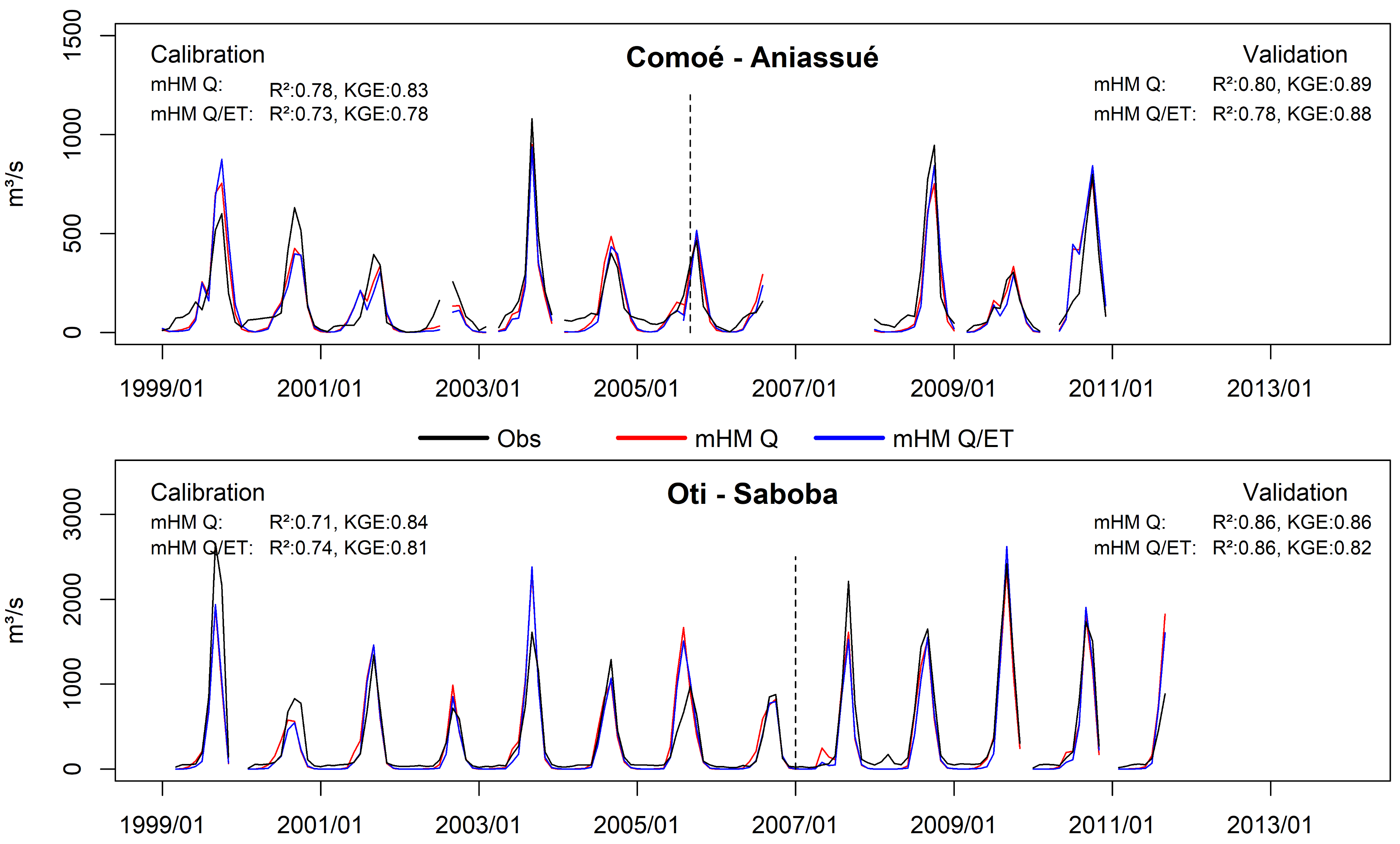
Two example hydrographs for the Comoé and Oti river basin calibration and validation are given in Figure 8. Displayed is the mean monthly observed and simulated discharge of the Q and Q/ET calibration schemes, as well as the respective key efficiency criteria (R2 and KGE). In both examples, Q and Q/ET model setups perform very well, with slightly higher KGE values reached by the Q model. As can be seen, performance of both models is higher during the validation period for these basins.
3.3. Multivariate Validation Results
Results of the two calibration approaches were further validated against actual evapotranspiration, soil moisture anomaly and total water storage anomaly data. Since mHM was set up to produce monthly output data (except for streamflow, which was daily), all validations are performed with monthly data. Results of the ETA validation are shown in Table 2 and Figure 9. For the Q calibration, the model overestimated ETA during the rainy seasons, but acceptable results are still reached. Compared against the three reference datasets, mHM performs best against GLEAM 3.2b, with an R2 of 0.93, 6.6% bias and a KGE of 0.73. Good results were also achieved when validating against GLEAM 3.2a, albeit with a slightly higher bias (8.1%) and lower, but still acceptable, KGE of 0.64. However, a marked difference could be seen compared to MODIS data, with a bias of 11.3% and a no longer acceptable KGE of 0.44. It can be observed that the amplitude of MODIS is lower than in the other products. On average, R2 is very good at 0.93 and bias is reasonable at 8.7%. Average KGE is still acceptable at 0.60. Results are markedly improved for the Q/ET calibration, but the order of validation performance is identical, even though GLEAM 3.2a was used as calibration input. Best validation is against GLEAM 3.2b, with an R2 of 0.97, 5.9% bias and a very good KGE of 0.93. Second highest validation occurs against GLEAM 3.2a (R2: 0.97; bias: 7.4%, KGE: 0.88) and the validation against MODIS, although in itself still good, performs worst of the three (R2: 0.92, bias: 10.7, KGE: 0.72). While the mean KGE strongly increases from 0.60 (Q) to 0.84 (Q/ET), mean RMSE decreases from 15.3 mm (Q) to 9.0 mm (Q/ET).
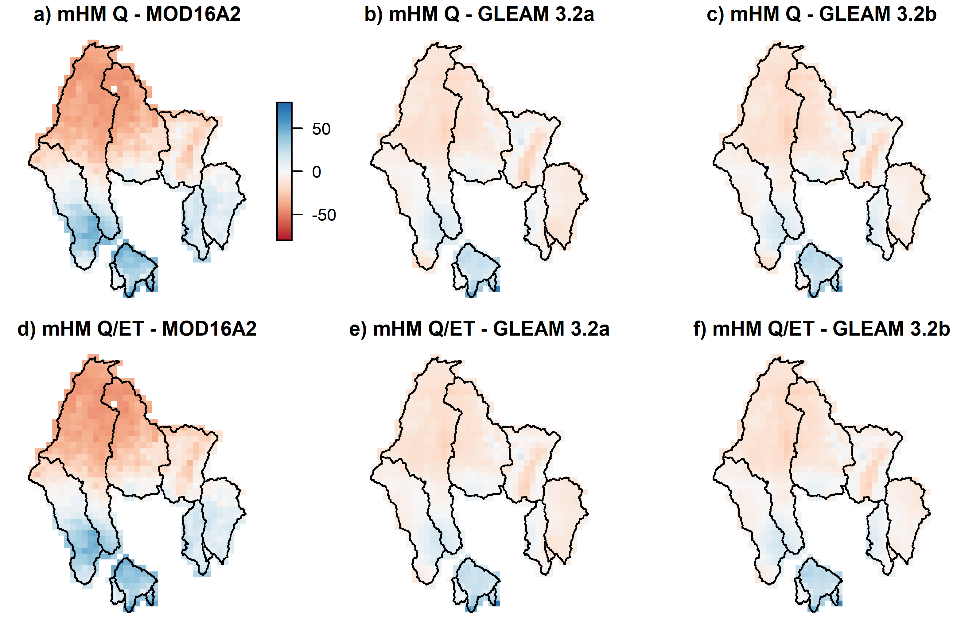
Figure 10 shows monthly mean raster comparison maps of model ETA against each of the validation datasets. The maps were produced by first resampling the remote sensing data to the mHM resolution, aggregating daily to monthly data and then subtracting mHM from remote sensing results for the period of data availability. Results indicate that mHM Q calibration-based ETA simulations and MODIS ETA compare well, especially in the central part of the study area, but results towards the very north of the Black Volta and White Volta basins show some overestimation. ETA is underestimated by mHM in the south of the Comoé and Black Volta basins. In the southern Ankobra, Pra and Ayensu basins, mHM did not manage to capture the ETA amounts of the MODIS data well, showing strong underestimations. While comparison against GLEAM 3.2a also performs less well in the south, results are altogether better than for MODIS with lower over- and underestimations. Comparisons against GLEAM 3.2b also show good correspondence, except in the very south. Spatial distribution of the Q/ET calibration results is similar, albeit with slightly lower over- and underestimations.
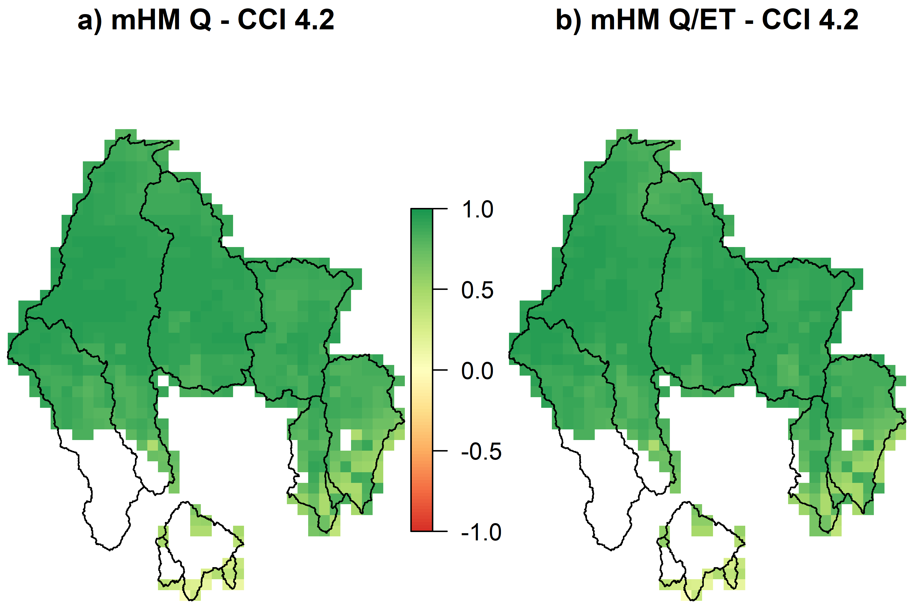
Both mHM calibration approaches capture the observed soil moisture anomalies well (Figure 11), reaching an R2 of 0.96, with a slightly better KGE performance of the Q/ET calibration (0.75) than the Q calibration (0.70). In both cases, mHM results show overestimation during the dry seasons and the Q/ET calibration shows an overall greater amplitude. Spatial correlations are high, as evident in Figure 12, except for weaker correlations in the south.
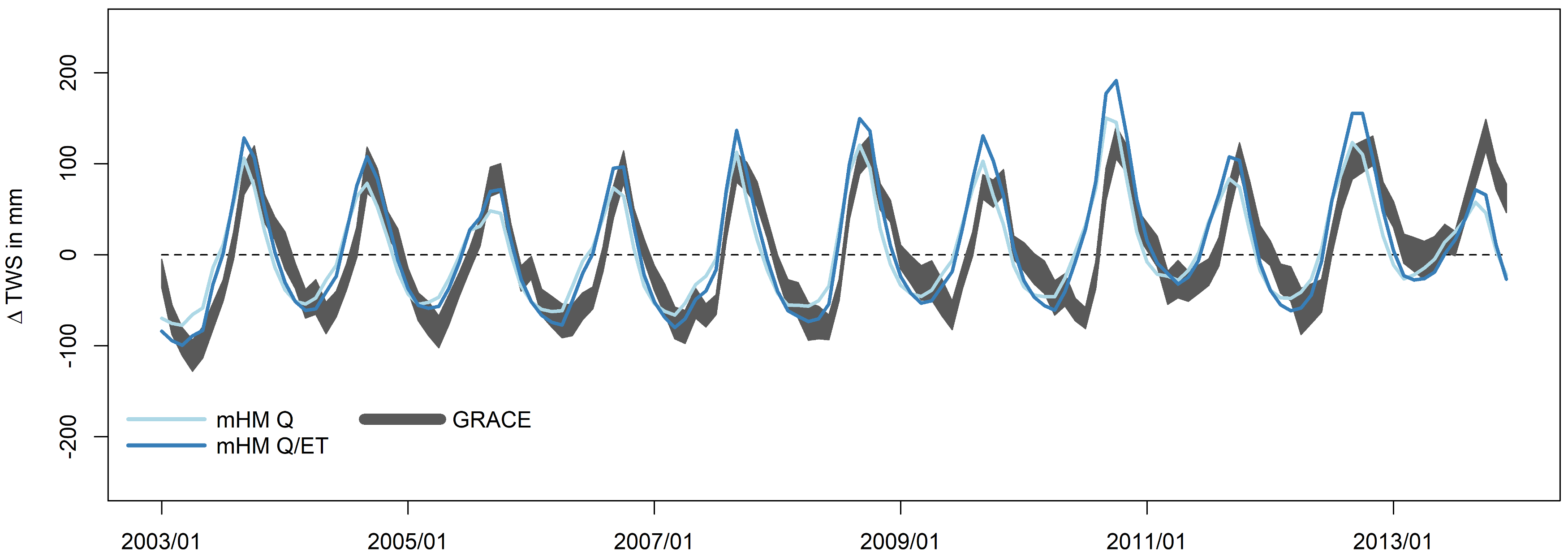
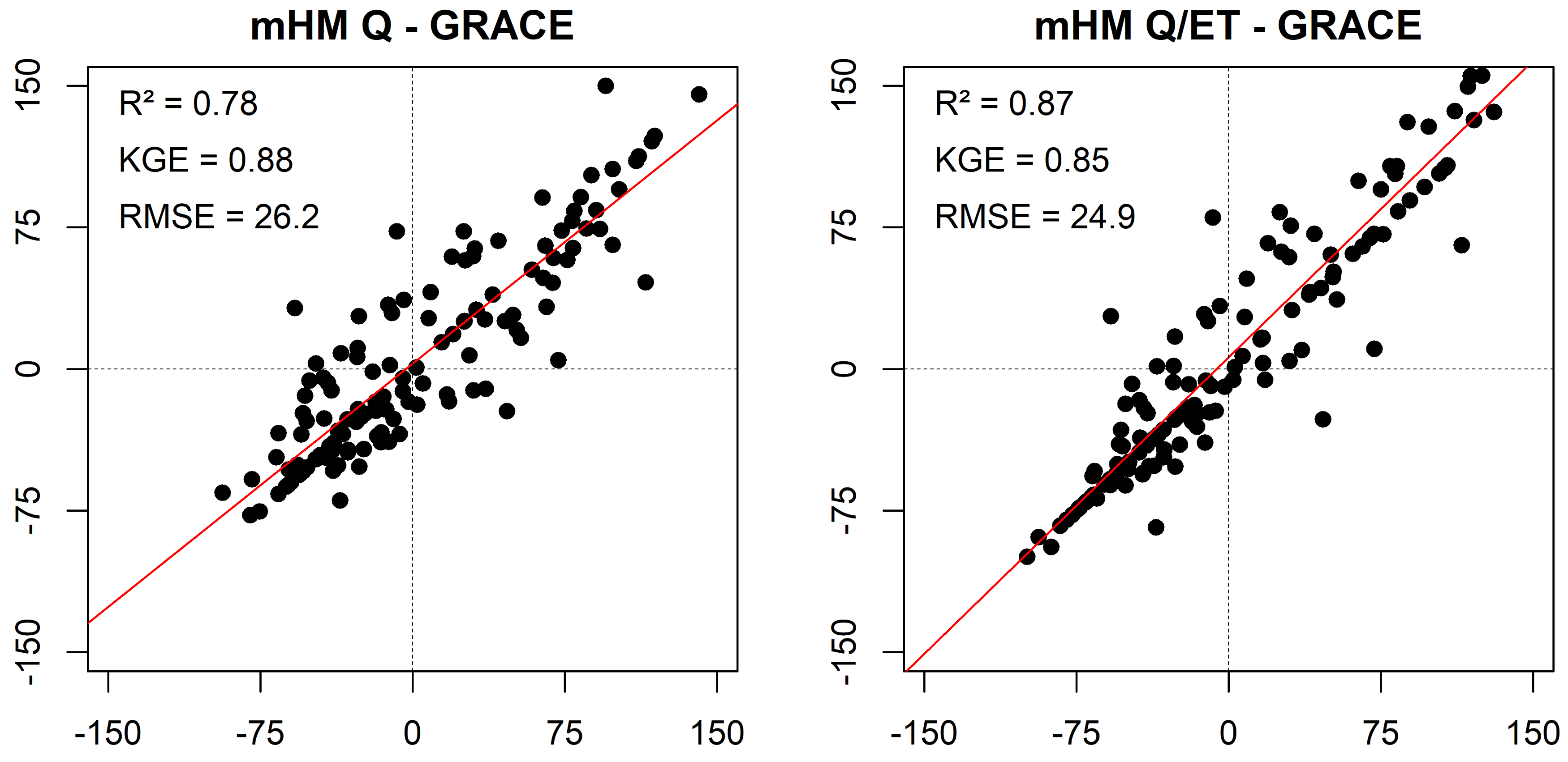
The simulated total water storage anomaly was evaluated against GRACE estimates. Results are shown in Figure 13 and Figure 14. Both model calibrations fit the ΔTWS estimation observed by GRACE well, but show a phase shift of approximately one month. The calibration approaches score a very good R2 of 0.78 for Q and 0.87 for Q/ET against GRACE retrievals. KGE is also very good at 0.88 and 0.85, while the root mean squared error is similar at 26.2 and 24.9 mm, respectively. Starting from 2008 onwards, a slight positive trend is established.
3.4. Evaluation of mHM-MPR for Transferability across Scales
After successful calibration of both Q and Q/ET models at a resolution of 26 km, the performance of the Multiscale Parameter Regionalization was evaluated by re-running the models under a different L1 output resolution with the calibrated optimal parameter sets. Results, depicted in Table 3, show the discharge simulation to remain stable during runs in finer resolutions of 13 and 6.5 km. While the results for both models remain identical for the calibrations (Q: 0.53, Q/ET: 0.49), validation results increase slightly from 0.23 to 0.28 (Q) and 0.13 to 0.17 (Q/ET). The number of modeled grid cells increases from 830 (26 km) to 3320 (13 km) and 13,280 (6.5 km), while the area per grid cell decreases from 676 to 169 and 42.3 km2. These results highlight the computational efficiency of the model, which can be calibrated at a coarse resolution and later run at a more resource-demanding, finer, resolution without introducing further bias.
4. Discussion
4.1. Initial Model Runs and Discharge Calibration and Validation
Results of the twelve exploratory model runs have shown ambiguity, depending on the combination of precipitation input and actual evapotranspiration calculation method. In our case, the use of ETA data with aspect correction based on the 500 m DEM was rejected outright, as it performed quite poorly, the exception being ETA and ΔTWS dynamics. While best uncalibrated streamflow results were achieved with the LAI correction method, it did not manage to sufficiently capture either ETP, nor ETA dynamics or amounts. The distribution of LAI classes has been dismissed as a factor, since selected LAI classes accurately depict a vegetation shift in line with the changing precipitation patterns from south to north. This leads us to question the quality of the ETP product used. Due to the period modeled, only the mostly reanalysis-based GLEAM 3.1a dataset was available, which uses ERA-Interim radiation and air temperature-, as well as MSWEP precipitation inputs to calculate ETP. [66]. The Hargreaves-Samani method produced the best ETP simulations. This method has also been proven to produce robust ETP estimations for the region in SWAT simulations and is preferred when data availability is limited or the quality in doubt [11,81]. Out of all precipitation products, CMORPH performed best in combination with the Hargreaves-Samani method. Due to equifinality, when calibrated, other datasets might perform similarly well. This has also been observed by Qi et al. [82] and Thiemig et al. [83], who both show product-specific model calibration to improve model results under various remote sensing precipitation inputs. Therefore, a multi-parameter validation is paramount to confirming the model robustness.
Calibration of the CMORPH and Hargreaves-Samani model using both Q and Q/ET as observed variables has shown the model to perform well for the region, leading to acceptable discharge simulations. However, some of the more northern stations in the Black and White Volta river basins perform poorly for both calibrations. The same is evident during the validations, where there are additional problems with several southern stations. Since the model performs well for other stations in the immediate vicinity, we attribute this to three main factors: (1) Data quality: Many stations show large gaps in the time-series or other inconsistencies. While obviously questionable data has been removed, performance might still be influenced. Especially in later years, data quality decreases while gaps increase. (2) Anthropogenic influences: mHM currently does not simulate reservoirs or water abstraction. Several reservoirs exist in the region, such as the Nangbeto reservoir in the southern Mono basin, upstream of the southernmost station, or the Bagre reservoir in the upper White Volta basin. Additionally, there are a multitude of smaller dams scattered mostly across the northern parts of the Black and White Volta basins in Burkina Faso [84]. (3) Calibration and validation periods: Due to having insufficient overlapping discharge timeseries, it was decided to run the model for the whole period and to use the first two thirds of the discharge records for calibration and the last third for validation. This approach allows the modeler to use all discharge records, even without overlap, and is opportune in basins with severely limited data availability [11,68]. In this approach, it can occur that data for several stations in a given basin is available for approximately the same period, while fewer stations have data for a different period. As the stations are equally weighted during optimization, this might negatively influence the results of the stations which are in the minority, especially under climatic anomalies.
4.2. Multivariate Validation and Scale Transferability of the mHM-MPR Scheme
In addition to discharge, actual evapotranspiration, soil moisture and total water storage anomalies were also validated. This allows the modeler to assess the robustness of the model [11,78]. According to the principle of equifinality, multiple parameter combinations lead to the same model result. Multi-parameter validation allows the modeler to check for inconsistencies or unrealistic behavior in the model and to rectify problems. This furthermore increases the model’s predictive capability, as confidence in the prediction of uncalibrated, but validated, variables is increased. During model calibration, it became obvious that if calibrated with default parameter ranges and discharge only, the model tends to remove surplus water into the atmosphere, leading to elevated ETA results. This was circumvented by restricting evapotranspiration parameters and opening infiltration parameters. The final result shows an overall good representation of ETA, although with some positive bias. Interestingly, when calibrated in combination with discharge and ETA, no such adjustment was necessary, and the model was able to find a sufficient solution within the default parameter ranges. While the streamflow performance decreased slightly for this method, ETA performance increased markedly. Both models perform better against GLEAM ETA (a and b) than against MODIS data; this is especially evident in the southern Comoé, as well as Ankobra, Pra and Ayensu river basins. Generally, MODIS estimates follow a similar dynamic but are lower than GLEAM estimates. MODIS data has also been reported to underpredict ETA in parts of South Africa [85,86]. GLEAM estimates show a single peak during the rainy season, while mHM and MODIS estimates tend to exhibit a longer period of maximum evapotranspiration for most years. Generally, mHM overestimates ETA in the north and underestimates in the south. This is more pronounced when compared to MODIS than to GLEAM data. Soil moisture anomalies are captured very well by both Q and Q/ET calibrations, with some slight overestimations during the wet seasons from 2006 to 2010. Other wet seasons are slightly underestimated. It is apparent that the model simulates a smaller loss of soil moisture in the dry season than CCI estimates. This might be because the upper soil layer simulated in mHM is 30 cm deep and will dry out significantly slower than the top few centimeters observed by satellites. While further horizons may be implemented in the model, it remains questionable whether model performance can be increased, since none of the soil physical parameters governing infiltration are available for the top few centimeters in the region.
Both Q and Q/ET model calibrations show a generally good agreement with GRACE total water storage estimates. mHM results appear to be slightly shifted by approximately one month. The same phenomenon has also been observed for other model simulations of the region [11,87,88]. The ΔTWS amplitude of the Q/ET calibration is greater than the Q calibration for all years. This can be attributed to the generally lower ETA estimates, leading to higher groundwater recharge in wet years and subsequently higher water storages during the wet seasons.
From 2008 to 2010, mHM tends to produce higher estimates than GRACE. Grippa et al. [87] come to the conclusion that incorrectly modeled evapotranspiration during the dry season may negatively influence TWS results. After comparing model and GRACE results for West Africa, Boone et al. [89], conclude that differences in amplitudes are due to either inaccuracies in the model precipitation forcing, deficiencies in the model structure, or the overestimation of the storage anomalies by GRACE. Ndehedehe et al. [88] hypothesize that land surface processes may be influenced anthropogenically, which is not sufficiently reflected in the model. Furthermore, they state that a lack of observed data for the region might lead to uncertain model predictions of soil moisture, and subsequently questionable TWS solutions. Some studies also indicate a clear positive trend towards higher water storage in the entire Volta basin from 2007 onwards, which is attributed mainly to an increase in precipitation [90,91,92]. This is only partly observed in our study. In Poméon et al. 2018 [11], we conclude that the strong signal of Lake Volta may mask TWS solutions. When the lake signal was removed during GRACE preprocessing, a positive trend was less obvious. Similar findings have been reported by Ndehedehe et al. [93], who observed a decline in TWS between 2007 and 2011 after removing the signal. Since only the upper Volta basins upstream of the lake were modeled in mHM, a TWS trend is also less evident.
In the context of multivariate calibration and validation, mHM has previously been shown to perform well when calibrated with SM and TWS [28,29]. However, applications have been limited to data-rich regions, e.g., Europe. Here we are considering the use of multivariate calibration and validation in a data-scarce domain to offset the poor availability of in situ data. Results show that using this approach, mHM produces reasonably realistic predictions even in these environments. It should however be considered that remote sensing estimates may themselves contain significant bias and generally should be validated for the specific region of interest. This is especially relevant for evapotranspiration products, where models are used to generate estimates based on satellite observations. In data-scarce regions, this proves especially challenging, and was neither conducted in this study, nor are the authors familiar with validations of the specific products for the study area. Studies conducted in Germany [40] and China [94] have also shown land surface temperature inputs to further constrain hydrologic model parameters.
Multiscale parameter regionalization has proven to perform well for discharge calibration and validation results under both Q and Q/ET calibrations. Calibration results are almost identical for all three resolutions, and validation results increase slightly for the finer resolutions. MPR seems to be a promising approach for reducing the runtimes of large-scale hydrologic models by calibrating at a computationally efficient coarse resolution and running the model in a significantly finer resolution. Scaling results obtained here are consistent with previous findings for EU and US regions [18,21,27,28].
5. Conclusion
In this study, we have proven mHM to perform reasonably well and to produce robust results for a (sparsely gauged) study area in southern West Africa. When considering the lack of in situ measurements in the region, the use of remote sensing data becomes a necessity to produce meaningful hydrologic predictions. The model has been developed for the express purpose of integrating these datasets. Running the uncalibrated model for twelve combinations of precipitation and evapotranspiration inputs and calculation methods has allowed us to rapidly screen the performance regarding each combination. This proved to be helpful in choosing the final model combination for further investigation. The model was first calibrated using discharge as the observed variable and then, to further reduce model uncertainty, calibrated using discharge and actual evapotranspiration data. Equifinality dictates that the same result can be achieved with an infinite combination of model parameters. Since some of these combinations may be unrealistic, the model may predict variables that were not included in the calibration poorly. It therefore becomes necessary to either include in the calibration, or to separately validate, all further variables of interest. This was performed using actual evapotranspiration, soil moisture anomaly and total water storage anomaly data. It has been shown that mHM can reasonably well predict discharge in the region. Further validation has confirmed actual evapotranspiration as well as soil moisture and total water storage anomaly predictions to perform well when compared to remote sensing products. When model parameters are further constrained using a calibration based on streamflow and actual evapotranspiration, the performance of the evapotranspiration simulation is vastly improved, while soil moisture and total water storage anomaly predictions remain stable. Discharge simulations, however, decrease in performance. Using Multiscale Parameter Regionalization, the calibrated model can then be run at a finer resolution while results remain stable. This approach is computationally efficient, as a calibration at a fine scale would take significantly longer to complete.
Further work is necessary to fully investigate the model uncertainty under different remote sensing inputs, as well as the performance of product-specific calibration for each of the considered precipitation datasets. Also, the contribution of land surface temperature to further constrain model parameters should be assessed. Since the remote sensing products have not been validated due to the lack of in situ data in the region, it would be interesting to assess the uncertainty between different datasets. This is especially relevant for datasets which rely on models to generate estimates. As a SWAT simulation has already been performed for the study area, a thorough model comparison will be conducted to assess the strengths of the individual models in the future. Due to the climate-data friendly nature of the model, climate scenarios can also be easily implemented.
Our modeling approach allows the modeler to build a robust hydrologic model relatively quickly by using only freely and easily available remote sensing and reanalysis data and software. This is especially interesting for predictions in sparsely gauged basins such as in West Africa, where the availability of data continues to decline. However, remote sensing should ideally be used to complement, and not replace, in situ measurements. We therefore firmly believe that there is a necessity for further investment into observation networks in West Africa.
Author Contributions
Conceptualization, T.P., B.D and R.K.; methodology, T.P., B.D. and R.K.; software, T.P and R.K; formal analysis, T.P., B.D. and R.K.; investigation, T.P.; writing—original draft preparation, T.P.; writing—review and editing, T.P., B.D. and R.K.; visualization, T.P.; supervision, B.D.; project administration, B.D.; funding acquisition, B.D.
Funding
This study is part of the COAST project (Studying changes of sea level and water storage for coastal regions in West Africa using satellite and terrestrial data sets) of the University of Bonn, supported by the Deutsche Forschungsgemeinschaft (German Research Foundation) under Grant No. DI443/6-1.
Acknowledgments
We thank Jürgen Kusche and Anne Springer of the Institute of Geodesy and Geoinformation, University Bonn, for providing the GRACE solutions. We are furthermore grateful to Christophe Peugeot and the AMMA-Catch project, as well as to the Global Runoff Data Centre in 56068 Koblenz, Germany for providing discharge data. The AMMA-CATCH regional observing system was set up thanks to an incentive funding of the French Ministry of Research that allowed pooling together various preexisting small-scale observing setups. The continuity and long term perenity of the measurements have been made possible by undisrupted IRD funding since 1990 and by a continuous CNRS-INSU funding since 2005.
Conflicts of Interest
The authors declare no conflict of interest.
Appendix A. mHM Parameters

| Parameter | Lower Threshold | Upper Threshold |
|---|---|---|
| Interception | ||
| canopyInterceptionFactor | 0.15 | 0.4 |
| Soil Moisture | ||
| orgMatterContent_forest | 0 | 20 |
| orgMatterContent_impervious | 0 | 1 |
| orgMatterContent_pervious | 0 | 4 |
| PTF_lower66_5_constant | 0.6462 | 0.9506 |
| PTF_lower66_5_clay | 0.0001 | 0.0029 |
| PTF_lower66_5_Db | −0.3727 | −0.1871 |
| PTF_higher66_5_constant | 0.5358 | 1.1232 |
| PTF_higher66_5_clay | −0.0055 | 0.0049 |
| PTF_higher66_5_Db | −0.5513 | −0.0913 |
| PTF_Ks_constant | −1.2 | −0.285 |
| PTF_Ks_sand | 0.006 | 0.026 |
| PTF_Ks_clay | 0.003 | 0.013 |
| rootFractionCoefficient_forest | 0.9 | 0.999 |
| rootFractionCoefficient_impervious | 0.9 | 0.95 |
| rootFractionCoefficient_pervious | 0.001 | 0.09 |
| infiltrationShapeFactor | 1 | 4 |
| Direct Sealed Area Runoff | ||
| imperviousStorageCapacity | 0 | 5 |
| Potential Evapotranspiration | ||
| minCorrectionFactorPET | 0.7 (0.9) | 1.3 (0.96) |
| maxCorrectionFactorPET | 0 (0.17) | 0.2 |
| aspectTresholdPET | 160 | 200 |
| HargreavesSamaniCoeff | 0.0016 (0.0021) | 0.003 (0.0027) |
| Interflow | ||
| interflowStorageCapacityFactor | 75 | 200 |
| interflowRecession_slope | 0 | 10 |
| fastInterflowRecession_forest | 1 | 3 |
| slowInterflowRecession_Ks | 1 | 30 |
| exponentSlowInterflow | 0.05 | 0.3 |
| Percolation | ||
| rechargeCoefficient | 0 | 50 (200) |
| Geological Parameter | ||
| GeoParam(1) | 1 | 1000 (1500) |
Given are the parameters calibrated in mHM and their standard ranges. Values in brackets signify modified ranges to improve actual evapotranspiration simulations of the Q calibration scheme. During the Q/ET calibration, default ranges were used. For further details, see [51] and www.ufz.de/mhm.
References
- Hollinger, F.; Staatz, J.M. Agricultural Growth in West Africa: Market and Policy Drivers; Hollinger, F., Staatz, J.M., Eds.; African Development Bank/Food and Agriculture Organization of the United Nations: Rome, Italy, 2015; ISBN 9789251087008. [Google Scholar]
- Jalloh, A.; Faye, M.D.; Roy-Macauley, H.; Sérémé, P.; Zougmoré, R.; Thomas, T.S.; Nelson, G.C. Overview. In West African Agriculture and Climate Change; Jalloh, A., Nelson, G.C., Thomas, T.S., Zougmoré, R., Roy-Macauley, H., Eds.; International Food Policy Research Institute: Washington, DC, USA, 2013. [Google Scholar]
- African Development Bank. West Africa Economic Outlook 2018; African Development Bank Group: Abidjan, Côte d’Ivoire, 2018; ISBN 9789938882667. [Google Scholar]
- Schuol, J.; Abbaspour, K.C.; Srinivasan, R.; Yang, H. Estimation of freshwater availability in the West African sub-continent using the SWAT hydrologic model. J. Hydrol. 2008, 352, 30–49. [Google Scholar] [CrossRef]
- Bormann, H. Regional hydrological modelling in Benin (West Africa): Uncertainty issues versus scenarios of expected future environmental change. Phys. Chem. Earth 2005, 30, 472–484. [Google Scholar] [CrossRef]
- Wagner, S.; Kunstmann, H.; Bárdossy, A.; Conrad, C.; Colditz, R.R. Water balance estimation of a poorly gauged catchment in West Africa using dynamically downscaled meteorological fields and remote sensing information. Phys. Chem. Earth 2009, 34, 225–235. [Google Scholar] [CrossRef]
- Fujihara, Y.; Yamamoto, Y.; Tsujimoto, Y.; Sakagami, J. Discharge Simulation in a Data-Scarce Basin Using Reanalysis and Global Precipitation Data: A Case Study of the White Volta Basin. J. Water Resour. Prot. 2014, 6, 1316–1325. [Google Scholar] [CrossRef]
- Schuol, J.; Abbaspour, K.C. Calibration and uncertainty issues of a hydrological model (SWAT) applied to West Africa. Adv. Geosci. 2006, 9, 137–143. [Google Scholar] [CrossRef]
- Schuol, J.; Abbaspour, K.C.; Yang, H.; Srinivasan, R.; Zehnder, A.J.B. Modeling blue and green water availability in Africa. Water Resour. Res. 2008, 44, 1–18. [Google Scholar] [CrossRef]
- Xie, H.; Longuevergne, L.; Ringler, C.; Scanlon, B.R. Calibration and evaluation of a semi-distributed watershed model of Sub-Saharan Africa using GRACE data. Hydrol. Earth Syst. Sci. 2012, 16, 3083–3099. [Google Scholar] [CrossRef] [Green Version]
- Poméon, T.; Diekkrüger, B.; Springer, A.; Kusche, J.; Eicker, A. Multi-Objective Validation of SWAT for Sparsely-Gauged West African River Basins—A Remote Sensing Approach. Water 2018, 10, 451. [Google Scholar] [CrossRef]
- Adjei, K.A.; Ren, L.; Appiah-Adjei, E.K.; Kankam-Yeboah, K.; Agyapong, A.A. Validation of TRMM Data in the Black Volta Basin of Ghana. J. Hydrol. Eng. 2012, 17, 647–654. [Google Scholar] [CrossRef]
- Hughes, D.A. Comparison of satellite rainfall data with observations from gauging station networks. J. Hydrol. 2006, 327, 399–410. [Google Scholar] [CrossRef]
- Arnold, J.G.; Moriasi, D.N.; Gassman, P.W.; Abbaspour, K.C.; White, M.J.; Srinivasan, R.; Santhi, C.; Harmel, R.D.; Van Griensven, A.; VanLiew, M.W.; et al. Swat: Model Use, Calibration, and Validation. ASABE 2012, 55, 1491–1508. [Google Scholar] [CrossRef]
- Arnold, J.G.; Srinivasan, R.; Muttiah, R.S.; Williams, J.R. Large area hydrologic modeling and assessment Part 1: Model development. J. Am. Water Resour. Assoc. 1998, 34, 73–89. [Google Scholar] [CrossRef]
- Srinivasan, R.; Ramanarayanan, T.S.; Arnold, J.G.; Bednarz, S.T. Large area hydrologic modeling and assessment part II: Model application. J. Am. Water Resour. Assoc. 1998, 34, 91–101. [Google Scholar] [CrossRef]
- Beven, K. Rainfall-Runoff Modelling: The Primer, 2nd ed.; Wiley-Blackwell: Chichester, UK, 2012; ISBN 9781119951001. [Google Scholar]
- Samaniego, L.; Kumar, R.; Attinger, S. Multiscale parameter regionalization of a grid-based hydrologic model at the mesoscale. Water Resour. Res. 2010, 46, 1–25. [Google Scholar] [CrossRef]
- Schulla, J.; Jasper, K. Model Description WaSiM-ETH (Water Balance Simulation Model ETH); ETH Zurich: Zurich, Switzerland, 2007; Volume 41. [Google Scholar]
- Beven, K. How far can we go in distributed hydrological modelling? Hydrol. Earth Syst. Sci. 2001, 5, 1–12. [Google Scholar] [CrossRef] [Green Version]
- Kumar, R.; Samaniego, L.; Attinger, S. Implications of distributed hydrologic model parameterization on water fluxes at multiple scales and locations. Water Resour. Res. 2013, 49, 360–379. [Google Scholar] [CrossRef]
- Orth, R.; Staudinger, M.; Seneviratne, S.I.; Seibert, J.; Zappa, M. Does model performance improve with complexity? A case study with three hydrological models. J. Hydrol. 2015, 523, 147–159. [Google Scholar] [CrossRef] [Green Version]
- Pokhrel, P.; Gupta, H.V.; Wagener, T. A spatial regularization approach to parameter estimation for a distributed watershed model. Water Resour. Res. 2008, 44, 1–16. [Google Scholar] [CrossRef]
- Beven, K.J. Prophecy, reality and uncertainty in distributed hydrological modelling. Adv. Water Resour. 1993, 16, 41–51. [Google Scholar] [CrossRef]
- Becker, A.; Braun, P. Disaggregation, aggregation and spatial scaling in hydrological modelling. J. Hydrol. 1999, 217, 239–252. [Google Scholar] [CrossRef]
- Kumar, R.; Samaniego, L.; Attinger, S. The effects of spatial discretization and model parameterization on the prediction of extreme runoff characteristics. J. Hydrol. 2010, 392, 54–69. [Google Scholar] [CrossRef]
- Kumar, R.; Livneh, B.; Samaniego, L. Toward computationally efficient large-scale hydrologic predictions with a multiscale regionalization scheme. Water Resour. Res. 2013, 49, 5700–5714. [Google Scholar] [CrossRef] [Green Version]
- Rakovec, O.; Kumar, R.; Mai, J.; Cuntz, M.; Thober, S.; Zink, M.; Attinger, S.; Schäfer, D.; Schrön, M.; Samaniego, L. Multiscale and Multivariate Evaluation of Water Fluxes and States over European River Basins. J. Hydrometeorol. 2016, 17, 287–307. [Google Scholar] [CrossRef]
- Rakovec, O.; Kumar, R.; Attinger, S.; Samaniego, L. Improving the realism of hydrologic model functioning through multivariate parameter estimation. Water Resour. Res. 2016, 52, 7779–7792. [Google Scholar] [CrossRef]
- Zink, M.; Kumar, R.; Cuntz, M.; Samaniego, L. A high-resolution dataset of water fluxes and states for Germany accounting for parametric uncertainty. Hydrol. Earth Syst. Sci. 2017, 21, 1769–1790. [Google Scholar] [CrossRef]
- Samaniego, L.; Kumar, R.; Zink, M. Implications of Parameter Uncertainty on Soil Moisture Drought Analysis in Germany. J. Hydrometeorol. 2013, 14, 47–68. [Google Scholar] [CrossRef]
- Thober, S.; Kumar, R.; Sheffield, J.; Mai, J.; Schäfer, D.; Samaniego, L. Seasonal Soil Moisture Drought Prediction over Europe Using the North American Multi-Model Ensemble (NMME). J. Hydrometeorol. 2015, 16, 2329–2344. [Google Scholar] [CrossRef]
- Kauffeldt, A.; Wetterhall, F.; Pappenberger, F.; Salamon, P.; Thielen, J. Technical review of large-scale hydrological models for implementation in operational flood forecasting schemes on continental level. Environ. Model. Softw. 2016, 75, 68–76. [Google Scholar] [CrossRef]
- Hattermann, F.; Krysanova, V.; Gosling, S.N.; Dankers, R.; Daggupati, P.; Donnelly, C.; Flörke, M.; Huang, S.; Motovilov, Y.; Buda, S.; et al. Cross-scale intercomparison of climate change impacts simulated by regional and global hydrological models in eleven large river basins. Clim. Chang. 2017, 141, 561–576. [Google Scholar] [CrossRef]
- Samaniego, L.; Kumar, R.; Breuer, L.; Chamorro, A.; Flörke, M.; Pechlivanidis, I.G.; Schäfer, D.; Shah, H.; Vetter, T.; Wortmann, M.; et al. Propagation of forcing and model uncertainties on to hydrological drought characteristics in a multi-model century-long experiment in large river basins. Clim. Chang. 2017, 141, 435–449. [Google Scholar] [CrossRef]
- Krysanova, V.; Vetter, T.; Eisner, S.; Huang, S.; Pechlivanidis, I.; Strauch, M.; Gelfan, A.; Kumar, R.; Aich, V.; Arheimer, B.; et al. Intercomparison of regional-scale hydrological models and climate change impacts projected for 12 large river basins worldwide—A synthesis. Environ. Res. Lett. 2017, 12, 105002. [Google Scholar] [CrossRef]
- Huang, S.; Kumar, R.; Flörke, M.; Yang, T.; Hundecha, Y.; Kraft, P.; Gao, C.; Gelfan, A.; Liersch, S.; Lobanova, A.; et al. Erratum to: Evaluation of an ensemble of regional hydrological models in 12 large-scale river basins worldwide (Climatic Change, 10.1007/s10584-016-1841-8). Clim. Chang. 2017, 141, 399–400. [Google Scholar] [CrossRef]
- Zink, M.; Samaniego, L.; Kumar, R.; Thober, S.; Mai, J.; Schäfer, D.; Marx, A. The German drought monitor. Environ. Res. Lett. 2016, 11, 074002. [Google Scholar] [CrossRef] [Green Version]
- Samaniego, L.; Kumar, R.; Jackisch, C. Predictions in a data-sparse region using a regionalized grid-based hydrologic model driven by remotely sensed data. Hydrol. Res. 2011, 42, 338–355. [Google Scholar] [CrossRef]
- Zink, M.; Mai, J.; Cuntz, M.; Samaniego, L. Conditioning a Hydrologic Model Using Patterns of Remotely Sensed Land Surface Temperature. Water Resour. Res. 2018, 54, 2976–2998. [Google Scholar] [CrossRef]
- Poméon, T.; Jackisch, D.; Diekkrüger, B. Evaluating the performance of remotely sensed and reanalysed precipitation data over West Africa using HBV light. J. Hydrol. 2017, 547, 222–235. [Google Scholar] [CrossRef]
- CILSS. Landscapes of West Africa—A Window on a Changing World; U.S. Geological Survey EROS: Garretson, SD, USA, 2016.
- Lehner, B.; Verdin, K.; Jarvis, A. HydroSHEDS Technical Documentation Version 1.2; World Wildlife Fund US: Washington, DC, USA, 2013. [Google Scholar]
- Lehner, B.; Verdin, K.; Jarvis, A. New global hydrography derived from spaceborne elevation data. Eos 2008, 89, 93–94. [Google Scholar] [CrossRef]
- Fink, A.H.; Christoph, M.; Born, K.; Bruecher, T.; Piecha, K.; Pohle, S.; Schulz, O.; Ermert, V. Climate. In Impacts of Global Change on the Hydrological Cycle in West and Northwest Africa; Speth, P., Christoph, M., Diekkrüger, B., Eds.; Springer: Heidelberg, Germany, 2010; pp. 54–58. [Google Scholar]
- Sebastian, K. Agro-Ecological Zones of Africa; International Food Policy Research Institute (Datasets): Washington, DC, USA, 2009. [Google Scholar]
- Gessner, U.; Niklaus, M.; Kuenzer, C.; Dech, S. Intercomparison of Leaf Area Index Products for a Gradient of Sub-Humid to Arid Environments in West Africa. Remote Sens. 2013, 5, 1235–1257. [Google Scholar] [CrossRef] [Green Version]
- Bergström, S. Global Perspectives on Loss of Human Life Caused by Floods; Swedish Meteorological and Hydrological Institute: Norrköping, Sweden, 1976. [Google Scholar]
- Bergström, S. The HBV Model—Its Structure and Applications; Swedish Meteorological and Hydrological Institute: Norrköping, Sweden, 1992; ISBN 0-918334-91-8. [Google Scholar]
- Liang, X.; Lettenmaier, D.P.; Wood, E.F.; Burges, S.J. A simple hydrologically based model of land surface water and energy fluxes for general circulation models. J. Geophys. Res. 1994, 99, 14415–14428. [Google Scholar] [CrossRef]
- Samaniego, L.; Brenner, J.; Cuntz, M.; Demirel, C.M.; Kaluza, M.; Kumar, R.; Langenberg, B.; Mai, J.; Rokovec, O.; Schäfer, D.; et al. The Mesoscale Hydrologic Model—Documentation for Verion 5.8; Helmholtz Centre for Environmental Research—UFZ: Leipzig, Germany, 2017. [Google Scholar]
- Livneh, B.; Kumar, R.; Samaniego, L. Influence of soil textural properties on hydrologic fluxes in the Mississippi river basin. Hydrol. Process. 2015, 29, 4638–4655. [Google Scholar] [CrossRef]
- Tolson, B.A.; Shoemaker, C.A. Dynamically dimensioned search algorithm for computationally efficient watershed model calibration. Water Resour. Res. 2007, 43, 1–16. [Google Scholar] [CrossRef]
- Behrangi, A.; Khakbaz, B.; Vrugt, J.A.; Duan, Q.; Sorooshian, S. Comment on “Dynamically dimensioned search algorithm for computationally efficient watershed model calibration” by Bryan, A. Tolson and Christine, A. Shoemaker. Water Resour. Res. 2008, 44, 2–4. [Google Scholar] [CrossRef]
- FAO/IIASA/ISRIC/ISS-CAS/JRC. Harmonized World Soil Database (Version 1.2); FAO: Rome, Italy; IIASA: Laxenburg, Austria, 2012. [Google Scholar]
- Bontemps, S.; Defourny, P.; Van Bogaert, E.; Arino, O.; Kalogirou, V.; Perez, J. GLOBCOVER 2009 Products Description and Validation Report; Université catholique de Louvain, European Space Agency: Louvain, Paris, 2011. [Google Scholar]
- Myneni, R.; Knyazikhin, Y.; Park, T. MCD15A2 MODIS/Combined Terra+Aqua Leaf Area Index/FPAR Daily L4 Global 1 km SIN Grid. Available online: https://ladsweb.modaps.eosdis.nasa.gov/missions-and-measurements/products/lai-and-fpar/MCD15A2/ (accessed on 1 August 2018).
- Knyazikhin, Y.; Glassy, J.; Privette, J.L.; Tian, Y.; Lotsch, A.; Zhang, Y.; Wang, Y.; Morisette, J.T.; Votava, P.; Myneni, R.B.; et al. MODIS Leaf Area Index (LAI) and Fraction of Photosynthetically Active Radiation Absorbed by Vegetation (FPAR) Product (MOD15) Algorithm Theoretical Basis Document. Available online: https://modis.gsfc.nasa.gov/data/atbd/atbd_mod15.pdf (accessed on 1 August 2018).
- Joyce, R.J.; Janowiak, J.E.; Arkin, P.A.; Xie, P. CMORPH: A Method that Produces Global Precipitation Estimates from Passive Microwave and Infrared Data at High Spatial and Temporal Resolution. J. Hydrometeorol. 2004, 5, 487–503. [Google Scholar] [CrossRef]
- Xie, P.; Yoo, S.; Joyce, R.; Yarosh, Y. Bias-Corrected CMORPH: A 13-Year Analysis of High-Resolution Global Precipitation. Available online: http://ftp.cpc.ncep.noaa.gov/precip/CMORPH_V1.0/REF/EGU_1104_Xie_bias-CMORPH.pdf (accessed on 13 March 2018).
- Huffman, G.J.; Bolvin, D.T.; Nelkin, E.J.; Wolff, D.B.; Adler, R.F.; Gu, G.; Hong, Y.; Bowman, K.P.; Stocker, E.F. The TRMM Multisatellite Precipitation Analysis (TMPA): Quasi-Global, Multiyear, Combined-Sensor Precipitation Estimates at Fine Scales. J. Hydrometeorol. 2007, 8, 38–55. [Google Scholar] [CrossRef]
- Ashouri, H.; Hsu, K.L.; Sorooshian, S.; Braithwaite, D.K.; Knapp, K.R.; Cecil, L.D.; Nelson, B.R.; Prat, O.P. PERSIANN-CDR: Daily precipitation climate data record from multisatellite observations for hydrological and climate studies. Bull. Am. Meteorol. Soc. 2015, 96, 69–83. [Google Scholar] [CrossRef]
- Schamm, K.; Ziese, M.; Raykova, K.; Becker, A.; Finger, P.; Meyer-Christoffer, A.; Schneider, U. GPCC Full Data Daily Version 1.0 at 1.0°: Daily Land-Surface Precipitation from Rain-Gauges Built on GTS-Based and Historic Data. Available online: ftp://ftp.dwd.de/pub/data/gpcc/html/fulldata-daily_v1_doi_download.html (accessed on 7 June 2016).
- Hargreaves, G.H.; Samani, Z.A. Reference Crop Evapotranspiration from Temperature. Appl. Eng. Agric. 1985, 1, 96–99. [Google Scholar] [CrossRef]
- Bosilovich, M.G.; Lucchesi, R.; Suarez, M. MERRA-2: File Specification. GMAO Office Note No. 9 (Version 1.1); NASA Goddard Space Flight Center: Greenbelt, MD, USA, 2016.
- Martens, B.; Miralles, D.G.; Lievens, H.; Van Der Schalie, R.; De Jeu, R.A.M.; Fernández-Prieto, D.; Beck, H.E.; Dorigo, W.A.; Verhoest, N.E.C. GLEAM v3: Satellite-based land evaporation and root-zone soil moisture. Geosci. Model. Dev. 2017, 10, 1903–1925. [Google Scholar] [CrossRef]
- Miralles, D.G.; Holmes, T.R.H.; De Jeu, R.A.M.; Gash, J.H.; Meesters, A.G.C.A.; Dolman, A.J. Global land-surface evaporation estimated from satellite-based observations. Hydrol. Earth Syst. Sci. 2011, 15, 453–469. [Google Scholar] [CrossRef] [Green Version]
- Abbaspour, K.C.; Rouholahnejad, E.; Vaghefi, S.; Srinivasan, R.; Yang, H.; Kløve, B. A continental-scale hydrology and water quality model for Europe: Calibration and uncertainty of a high-resolution large-scale SWAT model. J. Hydrol. 2015, 524, 733–752. [Google Scholar] [CrossRef]
- Liu, Y.Y.; Dorigo, W.A.; Parinussa, R.M.; De Jeu, R.A.M.; Wagner, W.; McCabe, M.F.; Evans, J.P.; Van Dijk, A.I.J.M. Trend-preserving blending of passive and active microwave soil moisture retrievals. Remote Sens. Environ. 2012, 123, 280–297. [Google Scholar] [CrossRef]
- Liu, Y.Y.; Parinussa, R.M.; Dorigo, W.A.; De Jeu, R.A.M.; Wagner, W.; Van Dijk, A.I.J.M.; McCabe, M.F.; Evans, J.P. Developing an improved soil moisture dataset by blending passive and active microwave satellite-based retrievals. Hydrol. Earth Syst. Sci. 2011, 15, 425–436. [Google Scholar] [CrossRef] [Green Version]
- Wagner, W.; Dorigo, W.; de Jeu, R.; Fernandez, D.; Benveniste, J.; Haas, E.; Ertl, M. Fusion of Active and Passive Microwave Observations To Create an Essential Climate Variable Data Record on Soil Moisture. ISPRS Ann. Photogramm. Remote Sens. Spat. Inf. Sci. 2012, 7, 315–321. [Google Scholar] [CrossRef]
- Gruber, A.; Dorigo, W.A.; Crow, W.; Wagner, W. Triple Collocation-Based Merging of Satellite Soil Moisture Retrievals. IEEE Trans. Geosci. Remote Sens. 2017, 55, 6780–6792. [Google Scholar] [CrossRef]
- Dorigo, W.; Wagner, W.; Albergel, C.; Albrecht, F.; Balsamo, G.; Brocca, L.; Chung, D.; Ertl, M.; Forkel, M.; Gruber, A.; et al. ESA CCI Soil Moisture for improved Earth system understanding: State-of-the art and future directions. Remote Sens. Environ. 2017, 203, 185–215. [Google Scholar] [CrossRef]
- Mu, Q.; Zhao, M.; Running, S.W. Improvements to a MODIS global terrestrial evapotranspiration algorithm. Remote Sens. Environ. 2011, 115, 1781–1800. [Google Scholar] [CrossRef]
- Mu, Q.; Heinsch, F.A.; Zhao, M.; Running, S.W. Development of a global evapotranspiration algorithm based on MODIS and global meteorology data. Remote Sens. Environ. 2007, 106, 285–304. [Google Scholar] [CrossRef]
- Mayer-Gürr, T.; Behzadpour, S.; Ellmer, M.; Kvas, A.; Klinger, B.; Zehentner, N. ITSG-Grace2016—Monthly and Daily Gravity Field Solutions from GRACE; TU Graz—Institute of Geodesy: Graz, Austria, 2016. [Google Scholar]
- Tapley, B.D.; Bettadpur, S.; Watkins, M.; Reigber, C. The gravity recovery and climate experiment: Mission overview and early results. Geophys. Res. Lett. 2004, 31, 1–4. [Google Scholar] [CrossRef]
- López, P.L.; Sutanudjaja, E.H.; Schellekens, J.; Sterk, G.; Bierkens, M.F.P. Calibration of a large-scale hydrological model using satellite-based soil moisture and evapotranspiration products. Hydrol. Earth Syst. Sci. 2017, 21, 3125–3144. [Google Scholar] [CrossRef] [Green Version]
- Gupta, H.V.; Kling, H.; Yilmaz, K.K.; Martinez, G.F. Decomposition of the mean squared error and NSE performance criteria: Implications for improving hydrological modelling. J. Hydrol. 2009, 377, 80–91. [Google Scholar] [CrossRef] [Green Version]
- Gavilán, P.; Lorite, I.J.; Tornero, S.; Berengena, J. Regional calibration of Hargreaves equation for estimating reference et in a semiarid environment. Agric. Water Manag. 2006, 81, 257–281. [Google Scholar] [CrossRef]
- Droogers, P.; Allen, R.G. Estimating reference evapotranspiration under inaccurate data conditions. Irrig. Drain. Syst. 2002, 16, 33–45. [Google Scholar] [CrossRef]
- Qi, W.; Zhang, C.; Fu, G.; Sweetapple, C.; Zhou, H. Evaluation of global fine-resolution precipitation products and their uncertainty quantification in ensemble discharge simulations. Hydrol. Earth Syst. Sci. 2016, 20, 903–920. [Google Scholar] [CrossRef] [Green Version]
- Thiemig, V.; Rojas, R.; Zambrano-Bigiarini, M.; De Roo, A. Hydrological evaluation of satellite-based rainfall estimates over the Volta and Baro-Akobo Basin. J. Hydrol. 2013, 499, 324–338. [Google Scholar] [CrossRef]
- Lehner, B.; Liermann, C.R.; Revenga, C.; Vörösmarty, C.; Fekete, B.; Crouzet, P.; Döll, P.; Endejan, M.; Frenken, K.; Magome, J.; et al. High-resolution mapping of the world’s reservoirs and dams for sustainable river-flow management. Front. Ecol. Environ. 2011, 9, 494–520. [Google Scholar] [CrossRef]
- Jovanovic, N.; Mu, Q.; Bugan, R.D.H.; Zhao, M. Dynamics of MODIS evapotranspiration in South Africa. Water SA 2015, 41, 79–91. [Google Scholar] [CrossRef]
- Sun, Z.; Gebremichael, M.; Ardö, J.; Nickless, A.; Caquet, B.; Merboldh, L.; Kutschi, W. Estimation of daily evapotranspiration over Africa using MODIS/Terra and SEVIRI/MSG data. Atmos. Res. 2012, 112, 35–44. [Google Scholar] [CrossRef]
- Grippa, M.; Kergoat, L.; Frappart, F.; Araud, Q.; Boone, A.; De Rosnay, P.; Lemoine, J.M.; Gascoin, S.; Balsamo, G.; Ottlé, C.; et al. Land water storage variability over West Africa estimated by Gravity Recovery and Climate Experiment (GRACE) and land surface models. Water Resour. Res. 2011, 47, 1–18. [Google Scholar] [CrossRef]
- Ndehedehe, C.; Awange, J.; Agutu, N.; Kuhn, M.; Heck, B. Understanding Changes in Terrestrial Water Storage over West Africa between 2002 and 2014. Adv. Water Resour. 2016, 88, 211–230. [Google Scholar] [CrossRef]
- Boone, A.; Decharme, B.; Guichard, F.; de Rosnay, P.; Balsamo, G.; Beljaars, A.; Chopin, F.; Orgeval, T.; Polcher, J.; Delire, C.; et al. The AMMA Land Surface Model Intercomparison Project (ALMIP). Bull. Am. Meteorol. Soc. 2009, 90, 1865–1880. [Google Scholar] [CrossRef] [Green Version]
- Forootan, E.; Kusche, J.; Loth, I.; Schuh, W.D.; Eicker, A.; Awange, J.; Longuevergne, L.; Diekkrüger, B.; Schmidt, M.; Shum, C.K. Multivariate Prediction of Total Water Storage Changes Over West Africa from Multi-Satellite Data. Surv. Geophys. 2014, 35, 913–940. [Google Scholar] [CrossRef] [Green Version]
- Rateb, A.; Kuo, C.-Y.; Imani, M.; Tseng, K.-H.; Lan, W.-H.; Ching, K.-E.; Tseng, T.-P. Terrestrial Water Storage in African Hydrological Regimes Derived from GRACE Mission Data: Intercomparison of Spherical Harmonics, Mass Concentration, and Scalar Slepian Methods. Sensors 2017, 17, 566. [Google Scholar] [CrossRef] [PubMed]
- Hassan, A.; Jin, S. Water storage changes and balances in Africa observed by GRACE and hydrologic models. Geod. Geodyn. 2016, 7, 39–49. [Google Scholar] [CrossRef]
- Ndehedehe, C.E.; Awange, J.L.; Kuhn, M.; Agutu, N.O.; Fukuda, Y. Analysis of hydrological variability over the Volta river basin using in-situ data and satellite observations. J. Hydrol. Reg. Stud. 2017, 12, 88–110. [Google Scholar] [CrossRef]
- Fang, Y.; Zhang, X.; Corbari, C.; Mancini, M.; Niu, G.; Zeng, W. Improving the Xin’anjiang hydrological model based on mass—Energy balance. Hydrol. Earth Syst. Sci. 2017, 21, 3359–3375. [Google Scholar] [CrossRef]
Figure 1.
(a) Study area with basins modeled in mHM; (b) Climate diagram Ouagadougou; (c) Climate diagram Cotonou. Dashed line indicates break in precipitation axis. Station data was compiled from the German Meteorological Agency Climate Data Center (DWD-CDC).
Figure 1.
(a) Study area with basins modeled in mHM; (b) Climate diagram Ouagadougou; (c) Climate diagram Cotonou. Dashed line indicates break in precipitation axis. Station data was compiled from the German Meteorological Agency Climate Data Center (DWD-CDC).

Figure 2.
Schematic overview of the mesoscale Hydrologic Model, mHM, developed at the Helmholtz Centre for Environmental Research—UFZ (Samaniego et al. 2017 [51]).
Figure 2.
Schematic overview of the mesoscale Hydrologic Model, mHM, developed at the Helmholtz Centre for Environmental Research—UFZ (Samaniego et al. 2017 [51]).

Figure 3.
Long-term (1999–2013) monthly sums of chosen precipitation inputs. Products were projected in the mHM L2 resolution and averaged over the study area.
Figure 3.
Long-term (1999–2013) monthly sums of chosen precipitation inputs. Products were projected in the mHM L2 resolution and averaged over the study area.

Figure 4.
Initial model evaluation simulation numbers. ETP method: chosen potential evapotranspiration method; HAR: Hargreaves-Samani; ASP: ETP read-in with aspect correction; LAI: ETP read-in with LAI correction.
Figure 4.
Initial model evaluation simulation numbers. ETP method: chosen potential evapotranspiration method; HAR: Hargreaves-Samani; ASP: ETP read-in with aspect correction; LAI: ETP read-in with LAI correction.

Figure 5.
Exploratory model results. Where CMORPH CRTv1, GPCC FDDv1, PERSIANN CDRv1 and TMPA 3B42v7 represent precipitation inputs; LAI, ASP and HAR are evapotranspiration calculation methods: HAR: Hargreaves-Samani; ASP: ETP read-in with aspect correction; LAI: ETP read-in with LAI correction; KGE: Kling-Gupta Efficiency; PBIAS: Percent bias; Q: Discharge; ETP: Potential evapotranspiration; ETA: Actual evapotranspiration; ΔTWS: Total water storage deviation from the mean.

Figure 6.
Discharge calibration and validation results, discharge (Q) calibration method.

Figure 7.
Discharge calibration and validation results, discharge and actual evapotranspiration (Q/ET) calibration method.
Figure 7.
Discharge calibration and validation results, discharge and actual evapotranspiration (Q/ET) calibration method.

Figure 8.
Example hydrographs for discharge (Q) and discharge and actual evapotranspiration (Q/ET) model calibrations. Daily model outputs have been aggregated to monthly data for visual clarity. Model efficiency calculations were performed on daily data.
Figure 8.
Example hydrographs for discharge (Q) and discharge and actual evapotranspiration (Q/ET) model calibrations. Daily model outputs have been aggregated to monthly data for visual clarity. Model efficiency calculations were performed on daily data.

Figure 9.
Monthly actual evapotranspiration validation averaged over study basins.

Figure 10.
Actual evapotranspiration comparison maps. Shown is the mean monthly deviation of mHM model results from remote sensing results in mm. Positive values signify an underestimation of mHM and negative values an overestimation.
Figure 10.
Actual evapotranspiration comparison maps. Shown is the mean monthly deviation of mHM model results from remote sensing results in mm. Positive values signify an underestimation of mHM and negative values an overestimation.

Figure 11.
Monthly soil moisture anomaly validation averaged over study basins.

Figure 12.
mHM soil moisture correlation against ESA-CCI 4.2. (a) mHM discharge calibration; (b) mHM discharge and actual evapotranspiration calibration. White color = no data.
Figure 12.
mHM soil moisture correlation against ESA-CCI 4.2. (a) mHM discharge calibration; (b) mHM discharge and actual evapotranspiration calibration. White color = no data.

Figure 13.
Mean monthly total water storage anomaly validation averaged over study basins.

Figure 14.
Linear regression of mean monthly mHM and GRACE total water storage anomaly averaged over study basins.
Figure 14.
Linear regression of mean monthly mHM and GRACE total water storage anomaly averaged over study basins.

Table 1.
mHM discharge results for both discharge and discharge and evapotranspiration calibration averaged over study basins.
Table 1.
mHM discharge results for both discharge and discharge and evapotranspiration calibration averaged over study basins.
| Objective Function | Discharge Stations | ||||||
|---|---|---|---|---|---|---|---|
| R2 | sig. | PBIAS | KGE | R2 ≥ 0.5 | KGE ≥ 0.5 | KGE ≥ 0.7 | |
| Q Calibration | |||||||
| Calibration | 0.61 | <0.001 | −8.8 | 0.53 | 83% | 75% | 39% |
| Validation | 0.65 | <0.001 | 12.9 | 0.23 | 75% | 53% | 39% |
| Average | 0.63 | 2.0 | 0.38 | 79% | 64% | 39% | |
| Q/ET Calibration | |||||||
| Calibration | 0.56 | <0.001 | −8.1 | 0.49 | 72% | 69% | 33% |
| Validation | 0.62 | <0.001 | 25.2 | 0.13 | 75% | 47% | 28% |
| Average | 0.59 | 8.5 | 0.31 | 74% | 58% | 31% | |
R2: coefficient of determination, sig.: significance, PBIAS: percent bias. KGE: Kling-Gupta Efficiency, Q Calibration: mHM calibrated using observed discharge, Q/ET Calibration: mHM calibrated using observed discharge and actual evapotranspiration.
Table 2.
mHM modeled actual evapotranspiration validation against remote sensing datasets averaged over study basins.
Table 2.
mHM modeled actual evapotranspiration validation against remote sensing datasets averaged over study basins.
| Dataset | Objective Function | ||||
|---|---|---|---|---|---|
| R2 | sig. | PBIAS | KGE | RMSE | |
| Q Calibration | |||||
| MOD 16A2 | 0.93 | <0.001 | 11.3 | 0.44 | 17.9 |
| GLEAM 3.2a | 0.93 | <0.001 | 8.1 | 0.64 | 14.8 |
| GLEAM 3.2b | 0.93 | <0.001 | 6.6 | 0.73 | 13.1 |
| Average | 0.93 | 8.7 | 0.60 | 15.3 | |
| Q/ET Calibration | |||||
| MOD 16A2 | 0.92 | <0.001 | 10.7 | 0.72 | 12.3 |
| GLEAM 3.2a | 0.97 | <0.001 | 7.4 | 0.88 | 7.9 |
| GLEAM 3.2b | 0.97 | <0.001 | 5.9 | 0.93 | 6.9 |
| Average | 0.95 | 8.0 | 0.84 | 9.0 | |
R2: coefficient of determination, sig.: significance, PBIAS: percent bias. KGE: Kling-Gupta Efficiency, Q Calibration: mHM calibrated using observed discharge, Q/ET Calibration: mHM calibrated using observed discharge and actual evapotranspiration.
Table 3.
mHM multiscale parameter regionalization results, pixel count, and pixel size comparison for selected resolutions.
Table 3.
mHM multiscale parameter regionalization results, pixel count, and pixel size comparison for selected resolutions.
| Spatial Resolution | |||
|---|---|---|---|
| 26 km | 13 km | 6.5 km | |
| Ø KGE Discharge | |||
| Calibration − Q | 0.53 | 0.53 | 0.53 |
| Calibration − Q/ET | 0.49 | 0.49 | 0.49 |
| Validation − Q | 0.23 | 0.26 | 0.28 |
| Validation Q/ET | 0.13 | 0.15 | 0.17 |
| Model Domain | |||
| Pixel Count | 830 | 3320 | 13,280 |
| Pixel Area | 676 km2 | 169 km2 | 42.3 km2 |
Q: mHM calibrated using observed discharge, Q/ET: mHM calibrated using observed discharge and actual evapotranspiration; Ø KGE: mean Kling Gupta Efficiency of all discharge gauges; discharge is averaged over study basins.
© 2018 by the authors. Licensee MDPI, Basel, Switzerland. This article is an open access article distributed under the terms and conditions of the Creative Commons Attribution (CC BY) license (http://creativecommons.org/licenses/by/4.0/).
Share and Cite
MDPI and ACS Style
Poméon, T.; Diekkrüger, B.; Kumar, R. Computationally Efficient Multivariate Calibration and Validation of a Grid-Based Hydrologic Model in Sparsely Gauged West African River Basins. Water 2018, 10, 1418. https://doi.org/10.3390/w10101418
AMA Style
Poméon T, Diekkrüger B, Kumar R. Computationally Efficient Multivariate Calibration and Validation of a Grid-Based Hydrologic Model in Sparsely Gauged West African River Basins. Water. 2018; 10(10):1418. https://doi.org/10.3390/w10101418
Chicago/Turabian StylePoméon, Thomas, Bernd Diekkrüger, and Rohini Kumar. 2018. "Computationally Efficient Multivariate Calibration and Validation of a Grid-Based Hydrologic Model in Sparsely Gauged West African River Basins" Water 10, no. 10: 1418. https://doi.org/10.3390/w10101418
Note that from the first issue of 2016, this journal uses article numbers instead of page numbers. See further details here.