Stationary and Non-Stationary Frameworks for Extreme Rainfall Time Series in Southern Italy


Department of Informatics, Modelling, Electronics and System Engineering, University of Calabria, 87036 Arcavacata di Rende (CS), Italy
*
Author to whom correspondence should be addressed.
Water 2018, 10(10), 1477; https://doi.org/10.3390/w10101477
Submission received: 16 August 2018
/
Revised: 11 October 2018
/
Accepted: 17 October 2018
/
Published: 19 October 2018
(This article belongs to the Section Hydrology)
Abstract
:This study tests stationary and non-stationary approaches for modelling data series of hydro-meteorological variables. Specifically, the authors considered annual maximum rainfall accumulations observed in the Calabria region (southern Italy), and attention was focused on time series characterized by heavy rainfall events which occurred from 1 January 2000 in the study area. This choice is justified by the need to check if the recent rainfall events in the new century can be considered as very different or not from the events occurred in the past. In detail, the whole data set of each considered time series (characterized by a sample size N > 40 data) was analyzed, in order to compare recent and past rainfall accumulations, which occurred in a specific site. All the proposed models were based on the Two-Component Extreme Value (TCEV) probability distribution, which is frequently applied for annual maximum time series in Calabria. The authors discussed the possible sources of uncertainty related to each framework and remarked on the crucial role played by ergodicity. In fact, if the process is assumed to be non-stationary, then ergodicity cannot hold, and thus possible trends should be derived from external sources, different from the time series of interest: in this work, Regional Climate Models’ (RCMs) outputs were considered in order to assess possible trends of TCEV parameters. From the obtained results, it does not seem essential to adopt non-stationary models, as significant trends do not appear from the observed data, due to a relevant number of heavy events which also occurred in the central part of the last century.
1. Introduction
Modelling of hydro-meteorological variables is an important topic in the hydrology field, and it plays a crucial role in estimation of design values, referred to assigned return periods [1]. In this context, the statistical approaches, which are usually adopted for this modelling, can be regrouped into two main classes: stationary and non-stationary models [2]. Both classes constitute a wide ensemble of choices for a user, as they allow for taking into account uncertainty sources and/or possible trends, which may characterize the specific time series under investigation [2].
In all the models belonging to the stationary class, the values of a random variable X are assumed as independent and identically distributed (iid) with a probability distribution , where is the parameters vector, invariant in time. Concerning the calculation of , the main source of uncertainty is constituted by extrapolation of the probability law beyond the range of observed values for X [3,4].
As regards the non-stationary class, the values of a random variable are independent but not identically distributed (i/nid), and the probability law is characterized by a parameters vector which is not constant, but it is a function of some covariates, usually only the time t [5,6,7]. Consequently, in this case, a further source of uncertainty is introduced, related to the assumed function linking parameters and the covariate t [8]. In fact, evaluation of design values for X also implies that the function remains valid for the entire future design period. Moreover, another important aspect is the ergodicity [2,9], that is the possibility to estimate the properties of a stochastic process from only one realization (the observed time series); if the process is non-stationary, then ergodicity cannot hold. Thus, possible trends should be derived from external sources, different from the time series of interest [2].
In any case, data integration (i.e., using information from other sources) is necessary [10]. In fact, the sample size N is usually insufficient in order to obtain a robust estimation of quantities related to high values of [11]. This insufficiency is even more penalizing for non-stationary approaches, where it is necessary to extrapolate not only towards values of greater than the observed frequencies, but also in time, along the future design period, on the basis of the assumed parametric trends [12].
Possible external sources of information can be the data in neighbor sites (by using regionalization techniques), or future scenarios derived from climate models [8]. However, this latter type of information should be used with great care, as it does not derive from observed series, but from outputs of models [2].
In this general context, the estimation of hydrological extremes, in future temporal horizons, presents high levels of uncertainty [3,4,13].
In the observed time series, the presence of some outliers can constitute an indicator of a non-stationary model, but these outliers sometimes occurred not only in the more recent years, thus making weaker the hypothesis of a presence of trends for some sites [14].
As an alternative to the hypothesis of a non-stationary model, the presence of outliers could be modelled by considering the imperfect knowledge of parameters (i.e., parameters are assumed as random variables with assigned probability distributions, [15]) and preserving the hypothesis of a stationary process. In this way, only the observed data of the specific site are used and, in a parsimonious framework, no further source of uncertainty is introduced if a parametric trend is not considered.
From all these briefly discussed aspects, the importance to carry out an investigation/strategy emerges, like that illustrated in this work. The procedure should firstly assess the applicability of models belonging to both classes for the case study of interest. Then, according to the principle of parsimony and the satisfaction of hypothesis tests, the second step is the choice of the “operational” model (which could not necessarily be the more complex one) for successive practical applications (as example, estimations of quantiles) [16].
In this work, the authors investigated both hypotheses (stationary and non-stationary) for some rainfall time series related to gauges located in the Calabria region (southern Italy). The authors selected the Calabria region as a study area, because from a previous work regarding this zone [17] in which only continuous daily data series of the period 1916–2006 were analyzed, no significant trends in number and magnitude of extreme events emerged, unlike other neighboring parts (Central Alps and Northern Italy [18,19]). This specific behavior, found for Calabria, was also detected for other parts in the Mediterranean area (for example, the Iberian Peninsula [20]), while a general decrease of annual and monthly precipitation can be asserted for the whole Mediterranean area [21]. In this work, the authors extended the investigation to annual maximum time series with sub-daily durations (1–24 h), and they carried out an analysis which is different from the application of non-parametric tests like Mann–Kendall, adopted in [17]. The adopted methodologies, for stationary and non-stationary frameworks, were based on the Two-Component Extreme Value (TCEV, [22]) probability distribution, which is the most applied for annual maximum data series in Calabria.
2. Material and Methods
2.1. Study Area
The analyzed time series (detailed in Section 2.2) are related to the rain gauge network located in the Calabria region (southern Italy), characterized by an area of about 15,000 km2 and a perimeter of about 800 km. It is surrounded by the Ionian (eastern coast) and Tyrrhenian (western coast) seas. Calabria presents a typical summer subtropical climate [17], also known as the Mediterranean climate. In detail, the Ionian part is mainly affected by warm currents from Africa, which induce high temperatures and heavy rainfall events with short duration; western air currents usually affect the Tyrrhenian part, where milder temperatures and many orographic rainfall events mainly occur; the inland zone is characterized by colder winters with snow and fresher summers with some rainfall events [23].
The mean annual precipitation (MAP) over the whole region is about 1000 mm and more than 80% of this amount is recorded in the season from October to April [24]. MAP varies from west to east side and between mountains and lowlands. Along the west coast, it averages about 900 mm and decreases to 700 mm along the northern part of the Ionian coast, and it is usually greater than 1100 mm above elevations of 500–800 m (but also below 500 m a.s.l. for some stations located in the southern part of the region), while it is less than 900 mm for valleys and for coastal areas [24].
In general, the western part of Calabria presents greater values of MAP, while the most extreme events with short durations occur in the eastern part, as it is exposed to more intense (but less frequent) cyclones from North Africa and the Balkans [24].
2.2. Case Studies
The authors focused attention on annual maximum rainfall series. In particular, daily and sub-daily (1–24 h) durations were investigated, and time series with recent heavy rainfall events, which occurred from 1 January 2000, were analyzed. In order to make reliable comparisons with heavy rainfall of the last century, the authors only considered time series with a sample size N > 40 data (with N clearly related to the whole data set for specific stations, and not only to the data from 2000 onwards). The annual maximum data series were downloaded from the website of the Multi Risks Center of Calabria Region (www.cfd.calabria.it).
The list of the examined rain gauge time series is detailed in Table 1 (see also Figure 1 for the geographical location), in which the mean annual precipitation (MAP), the elevation, the sample size N, the analyzed durations, and the intensity and occurrence date of heavy rainfall events before and after 1 January 2000 are indicated for each investigated time series. Fourteen time series from 11 rain gauges were analyzed (for 3 stations, the authors investigated time series related to two different durations); 10 rain gauges out of 11 are located in the southern part of Calabria, from which 5 are in the Ionian zone, 4 in the central part, and 1 in the Tyrrhenian zone.
It can be observed that all the heavy rainfall accumulations, selected from 1 January 2000 for the 11 investigated rain gauges, belong to nine spatial storm events that occurred in Calabria (9–10 September 2000, 29–30 September 2000, 3 July 2006, 12 December 2008, 25 September 2009, 22 November 2011, 19 November 2013, 31 October–1 November 2015, 25–26 November 2016): seven out of nine happened in the autumn season September–October–November (SON), one in the summer season June–July–August (JJA), and one in the winter season December–January–February (DJF) (see MetOffice classification of meteorological seasons for more details, www.metoffice.gov.uk).
Concerning rainfall intensity, 130.2 mm in 1 h registered in Vibo Valentia (ID code 2800) on 3 July 2006 represents the highest value among the recent events. Focusing on percentages of MAP, 430.2 mm in 24 h occurred in Ardore Superiore (ID code 2210), constitutes the maximum observed rate (about 46% of MAP = 928.7 mm), and it is also the highest value registered in 24 h from 1 January 2000.
Moreover, within the analyzed time series (specifically, in 9 out of 14) there are rain data, observed in the last century, with a magnitude that is comparable with the recent heavy rainfall values, and they belong to 14 spatial storm events that occurred in the region (10 November 1932, 5 December 1933, 21 October 1935, 21 November 1935, 2 December 1938, 9 September 1939, 22 January 1946, 16–21 October 1951, 3 November 1953, 12 September 1958, 23 November 1959, 22 September 1965, 25 November 1993, 3 October 1996). Eleven events out of 14 occurred in SON season, while 2 events occurred in DJF season. Furthermore, for three time series, the maximum value observed in the last century is even higher than that recorded from 2000 to date: 325.1 mm in 1 day in Vibo Valentia (2 December 1938), 512 mm in 24 h in Chiaravalle Centrale (16 October 1951), and 637.9 mm in 24 h in Santa Cristina d’Aspromonte (16 October 1951).
From analysis of Table 1, it is clear that the almost all the heavy rainfall events (both recent and past) occurred during the SON season, in which there is mainly the development of large-scale storms coming from the lee of the Alps or the western Mediterranean for the Tyrrhenian zone, and from North Africa or the Balkans for the Ionian zone [24].
2.3. Theoretical Background of the Adopted Frameworks
A Cumulative Density Function (CDF) of a random variable X can be usually indicated as or (or when parametric trends are introduced), in an indistinct way.
However, a user should pay attention when is not assumed as deterministic but as a random vector, with an assigned joint density distribution . In this case, for a stationary approach, the following relationship is obtained by applying the total probability law:
and, in a similar way, for the non-stationary case:
Concerning Equation (2), the authors only considered a deterministic parametric trend in this work, in order to obtain a truly non-stationary model. In fact, “fluctuations of the parameters should generate stationary compound or mixed distributions” [2,25,26,27]. Consequently, for a deterministic the joint probability corresponds to the Dirac’s function , and Equation (2) can be simplified as:
Obviously, a similar simplification can be obtained for Equation (1), when is considered as deterministic and then is also in this case equal to , that means .
Overall, starting from the general Equations (1) and (3), it is possible to obtain several models, depending on the assumed expression for the probability distribution , on the deterministic or stochastic nature of parameters, and on the eventual presence of the parameters’ trend (which implies other assumptions, as explained in Section 2.3.3.).
2.3.1. The TCEV Distribution
In this work, the Two-Component Extreme Value (TCEV, [22]) distribution was adopted, which is very suitable for a regionalization approach and considers two independent processes, both having a Poisson rate of occurrence and an exponential distribution of magnitudes above a threshold. From these assumptions, it is possible to demonstrate that the CDF of the annual maximum X, deriving from these two processes, is [22]:
where . Label 1 is referred to the frequent events, while label 2 is associated to the outlier events. (i = 1, 2) represents the mean annual number of events (with clearly ) and (i = 1, 2) is the mean value of magnitudes (with clearly ). By fixing (i = 1, 2), Equation (4) can be rewritten as a product of two EV1 CDFs:
with .
A third equivalent expression for TCEV distribution, that is the most used in applications, is obtained by introducing two dimensionless parameters:
which allow the rewriting of Equation (4) as:
with , or, in an equivalent way on the basis on the index approach [28], as:
with ; is the expected value E[X] and is a function depending on , , :
in which Г(.) is the complete gamma function [29].
The couple (,) determines the theoretical skewness γ1 of TCEV [30]; from the triad (, ,) it is possible to calculate the CV (coefficient of variation).
As TCEV distribution is characterized by four parameters, their estimation from an at-site data series is robust enough if the sample has an adequate size N (at least 90–100 data). On the contrary, if N is less than 90 data, a regionalization approach is necessary, that means TCEV distribution is hierachically developed into three regional levels, explained below.
In the 1st level (40 < N < 90 data), and (and consequently γ1) are assumed as constant into defined homogeneous regions, while and (or ) are at-site estimated.
In the 2nd level (10 < N < 40 data), homogeneous sub-regions are also considered, within each region identified in the previous level. In each sub-region, besides the constancy of , (and then γ1) of the related region, the parameter is also assumed theoretically invariant from site to site, and thus CV is constant too. In this case, only one parameter ( or ) is at-site estimated.
In the 3rd level (N < 10 data), (or ) is also estimated in a regional way, by adopting defined empirical formulas, depending (in the case of rainfall) on the altitude of the point or other topographic covariates [31].
Several approaches for estimating TCEV regional parameters were developed. We can mention: a maximum likelihood procedure (TCEV-ML, [22,32]); a probability-weighted moments procedure (TCEV-PWM, [11]); a methodology using the Principle of Maximum Entropy (TCEV-POME, [33]).
For the selected case study, concerning annual maxima of daily and sub-daily rainfall accumulation, from application of TCEV-ML, the whole Calabria region is a unique homogenous region, and it is subdivided into three homogeneous sub-regions, named Tyrrhenian (T), Central (C), and Ionian (I), respectively, as shown in Figure 1. The regional values of parameters , and are reported in Table 2 [34].
2.3.2. Stationary Framework
For all the time series listed in Section 2.2, the authors considered two models belonging to the stationary framework.
The first is indicated as Model 1. It is the simplest version of Equation (1), in which , that means is deterministic and then . In this case, the authors assumed and the first level of regionalization for parameter estimation was used (as only time series with N > 40 data were analyzed).
The second is denoted as Model 2, and it represents the complete version of Equation (1), in which is computed as described below.
First of all, in order to evaluate the joint probability distribution in Equation (1), the authors used the expression related to Equation (10), that means , and then the expected value (for each analyzed time series with N > 40) was assumed as deterministic and equal to the sample mean. Consequently, and then attention was focused on the marginal distributions , and .
As regards and , let a standardized random variable be defined as:
For each considered value of N (40, 50, …, 500), 1000 synthetic samples of were generated with a Monte Carlo approach by using Equation (13) and the regional values of and , as reported in Table 2. For each synthetic sample, estimations of and , indicated as and , were carried out by applying a ML procedure [22,32], and then empirical distributions for and were obtained, depending on N, and assumed as valid for the whole homogenous region.
Regardless of N, the normal and log-normal distributions showed the best fitting for and , respectively, as shown in Figure 2 and Figure 3, and the median values were, in any case, equal to the assumed theoretical values and , respectively (for the latter correspondence, please refer to [35], p. 216).
Concerning the standard deviations and , a clear and expected dependence on N emerged, as shown in Figure 4.
Analyzing the dispersion plot in Figure 5, obtained with all the values and estimated from all the synthetic series, and were assumed as independent random variables.
As regards , it was theoretically derived ([35], p. 237): as corresponds to the mean value of a distribution (Poisson in this case), its distribution is close to normal if N > 30 data even when the original variable is not normally distributed. Further theoretical results are:
where is the theoretical standard deviation of the original (Poisson) distribution.
Consequently, for a time series with a sample size N, the authors considered the sub-region where the rain gauge is placed, and then they used the associated regional value , as shown in Table 2, in order to compute the normal distribution with parameters expressed by Equations (14) and (15).
Moreover, was also assumed as independent on both and , and thus was set equal to the product , where and are the normal and log-normal, respectively, distributions explained above and assumed as valid for the whole Calabria region.
2.3.3. Non-Stationary Framework
The whole procedure, described below, is indicated by the authors as Model 3. Because of violation of ergodicity when a process is non-stationary [2], the authors used information external from the data series of rain gauges for non-stationary analysis. The report of the European Environmental Agency (EEA) [36] and the publication of the Italian Institute for Environmental Protection and Research (ISPRA) [37] were examined, concerning analysis of future climate in Europe and Italy, respectively, by using projections from Regional Climate Models (RCMs). Four RCMs were adopted (named as ALADIN, GUF, CMCC, LMD) and, for each one, four scenarios of Representative Concentration Pathways (RCPs) of total radiative forcing (i.e., cumulative measure of human emissions of greenhouse gasses from all sources expressed in W/m2) were used as input: RCP 2.6, RCP 4.5, RCP 6, and RCP 8.5. Moreover, an ensemble mean projection from all the RCMs is also derived for each RCP.
Focusing the attention on RCP 4.5 (intermediate emissions) and RCP 8.5 (high emissions), with respect to the reference period 1971–2000, the results of the simulations, related to a future period until 2090 for the Calabria region, can be summarized as indicated below.
A modest increase is predicted for the annual maximum daily rainfall. The ensemble mean is, for both RCP 4.5 and RCP 8.5, up to 10 mm, with a maximum increase of 35–40 mm from the CMCC model.
On the contrary, a significant increase for the waiting time between two consecutive rainfall events is forecasted. The ensemble mean is: up to 15 days for RCP 4.5, with a maximum increase of 30 days from the CMCC model; up to 30 days for RCP 8.5, with a maximum increase of 40 days from the CMCC model.
It has to be highlighted that these results are, obviously, affected by uncertainties, derived from the structure of the adopted numerical schemes of RCMs, and from their spatial and temporal resolutions. In fact, RCMs generally underestimate extreme precipitation intensity, and they are better at locating an extreme rainfall event than estimating its intensity. Model accuracy clearly improves with resolution, but RCMs with spatial resolution between 10 and 30 km, typically used in climate change studies, are still too coarse to explicitly represent sub-daily localized heavy precipitation events [38,39]. A very high-resolution model (typically 1–5 km), used for weather forecasts with explicit convection, has recently used for a climate change experiment for a region in the UK: this study projects an intensification of short duration heavy rain in summer, with significantly more events exceeding the high thresholds indicative for serious flash flooding [38,40,41].
However, on the basis on these results, the non-stationary framework was organized by the authors by considering the features associated to the outliers (i.e., the parameters with label 2 in Equation (4)). In detail, the authors established a positive trend for and a negative trend for .
Clearly, the specific mathematical expression for the parameters’ trend constitutes a not negligible source of uncertainty in a non-stationary framework. In this context, several expressions could be assumed [2]: linear, quadratic, regime shifts, sequence of different forms, etc.
In this work, the authors assumed the following expressions:
where is the year when the trend is supposed to begin, and are the rates of increase/decrease in one year for and , respectively, while and are the steady values of parameters before the beginning of the trend.
The authors set equal to 1980 (i.e., a year representative of the period when the scientific community began to discuss climate changes and the first conferences were organized) and to 2000 (i.e., the last year of the reference period for RCMs).
As regards and , their values were fixed in order to reach an increase/decrease in 100 years with the same order of magnitude of RCMs scenarios forecasted for the Calabria region; consequently, the authors set = 0.005 (i.e., an increase of 50% in 100 years) and = −0.002 (i.e., a decrease of 20% in 100 years). Finally, and were assumed as the estimations obtained by considering the time series as stationary until .
Overall, two versions were considered, depending on the assumed value for : Model 3_1980 and Model 3_2000. In detail, for a time series with N > 40, all the data which occurred when were used to estimate the stationary vector , by using a suitable level of regionalization, and the authors calculated and with Equations (7) and (8). Then, for each year , and holds from Equations (16) and (17), and the parameters vector for TCEV is , with and .
For large values of sample size N, the stationary parameter vector of Model 3 is usually very close to be identical to that associated to Model 1, when a user adopts a maximum likelihood (ML) procedure for parameter estimation (like in this work); in fact, ML application provides parameter values which are not so influenced by the presence of outliers.
2.3.4. Procedure for Models Application
For each time series, the authors tested all the previously described models.
As regards to Model 1, starting from Equation (9) with estimated at first level of regionalization, 1000 synthetic samples (with the same N of the observed series) were generated by using the Monte Carlo method. Then, for each synthetic sample, all the generated data were sorted in ascending order and assigned to specific Plotting Position (PP) values, calculated with Weibull formula [42]. It is clear that synthetic samples with the same N present the same set of PP values. Moreover, for each PP value, the 95% Confidence Intervals (CIs) of rainfall accumulation was derived and then the authors checked if the whole observed sample fell inside 95% CIs on an EV1 probabilistic plot; if the check is positive, the hypothesis of a stationary TCEV with as deterministic cannot be rejected.
Concerning Model 2, the authors considered Equation (10), with μ equal to the sample mean, while as random variables with probability distributions which are described in Section 2.3.2 (normal for and log-normal for ) and clearly depend on the value of sample size N. One thousand synthetic triads were derived with the Monte Carlo method, and each triad was used (togheter with μ) in Equation (10) to generate a specific sample with the same N of the observed series. Also in this case (with the same procedure of the previous Model 1), the observed data were compared with the estimated 95% CIs on an EV1 probabilistic plot, in order to evaluate the possibility of rejection or not for Model 2.
Referring to Model 3, as mentioned in Section 2.3.3, the authors assumed Equations (16) and (17) for trends regarding . Also in this case, the authors carried out a generation of 1000 synthetic samples (with the same N of the observed series) by using the Monte Carlo method, but considering (unlike Model 1) parameters vector as stationary until , and variable for . The check of rejection or not for Model 3 comprised the following two conditions: (i) all the occurred events when are inside the 95% CIs of Model 3 (which are estimated in a similar way to those of Models 1 and 2); (ii) all the occurred events when are inside the 95% CIs of the stationary component of Model 3 (which are very close to those of Model 1, for the reasons detailed at the end of Section 2.3.3). Only if both conditions are satisfied, then the validity of Model 3 cannot be rejected.
3. Results and Discussion
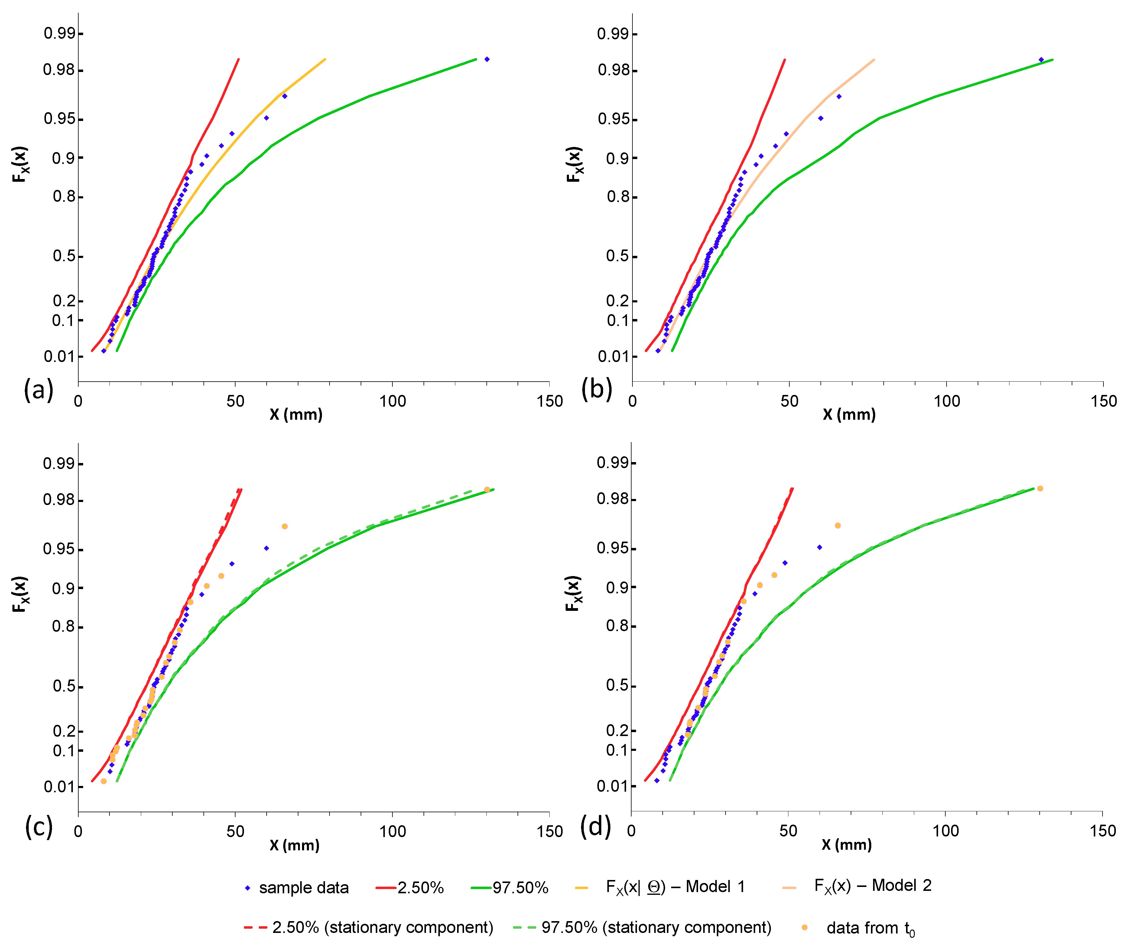
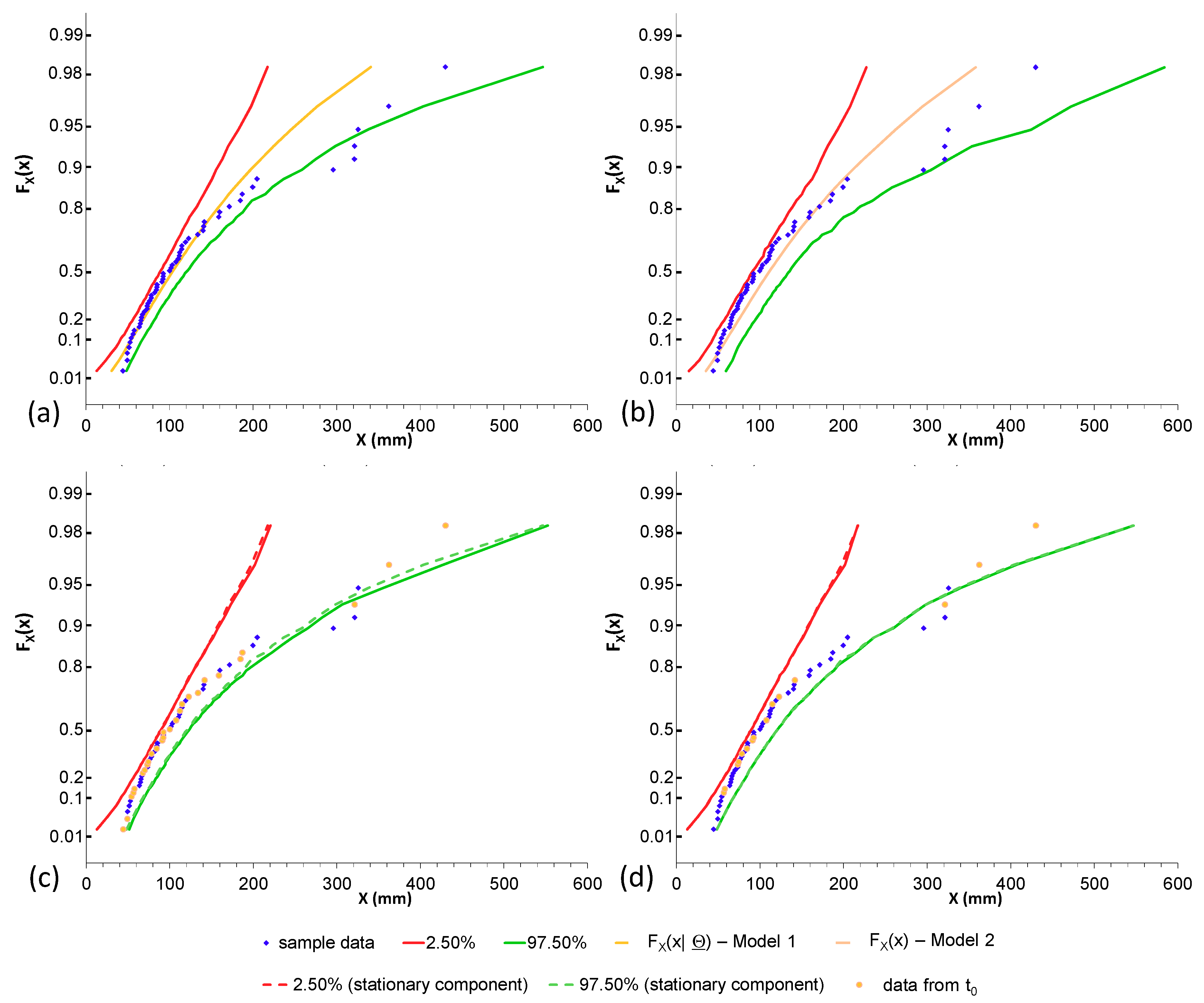
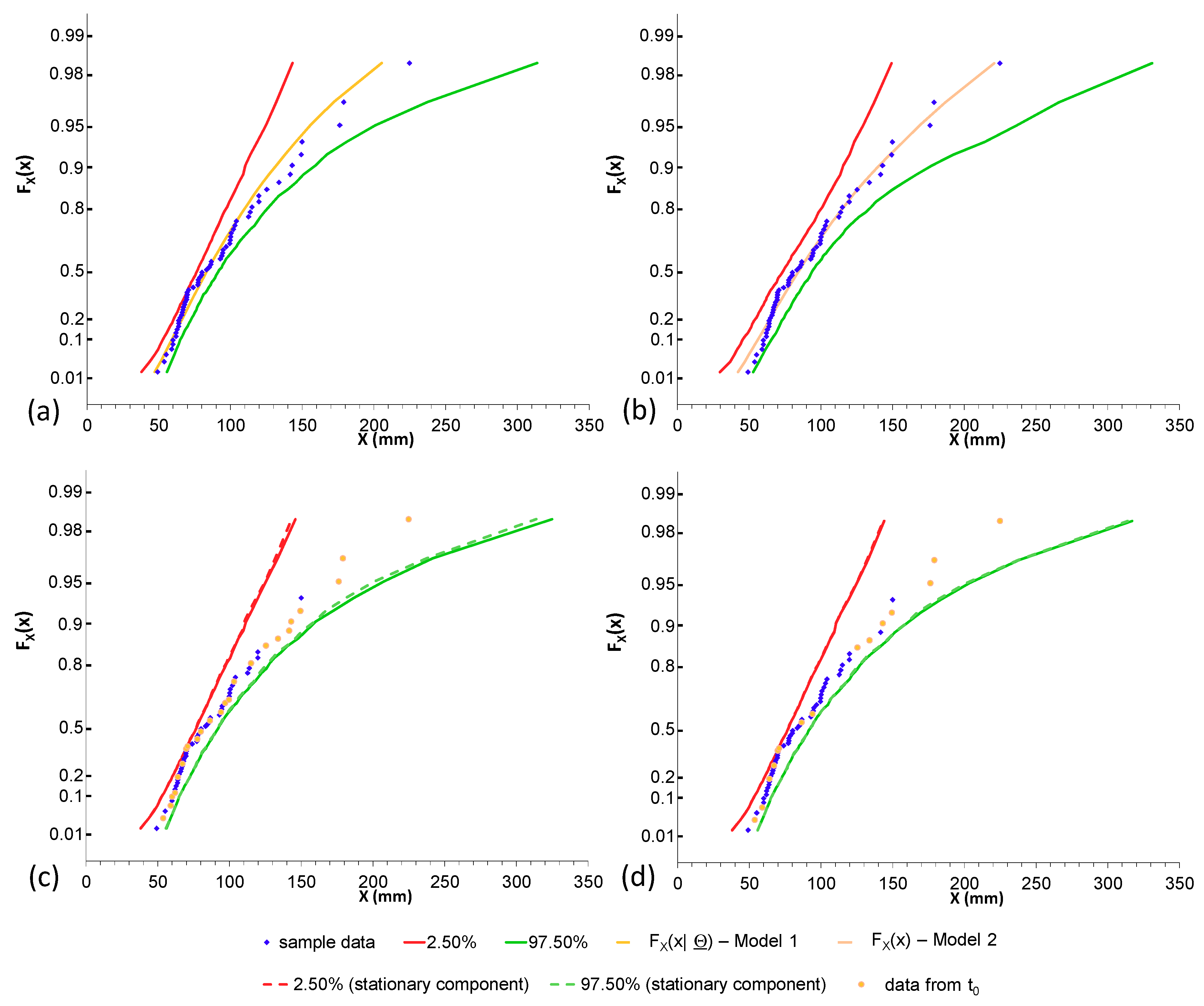
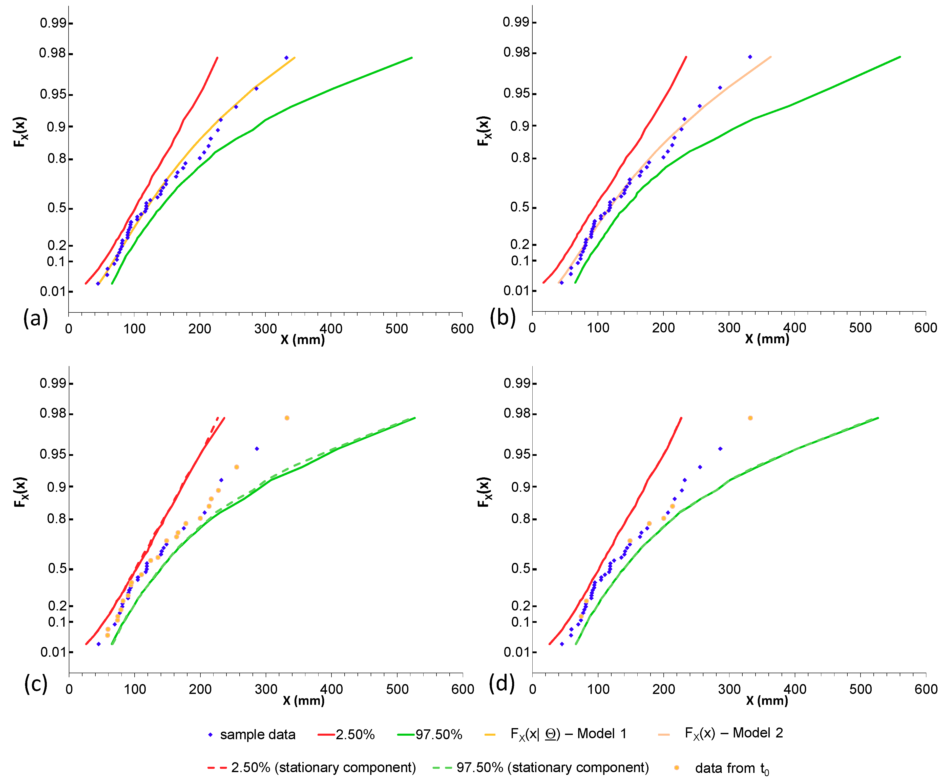
For all the time series, the obtained results on EV1 probabilistic plots are reported in Appendix A. In this section, as examples, the outcomes related to Vibo Valentia (1-h and daily time series) and Ardore Superiore (1-h and 24-h time series) are shown in Figure 6, Figure 7, Figure 8 and Figure 9.
Concerning the Vibo Valentia rain gauge, Model 1 is not able to reproduce, for both 1-h and daily durations, the outliers are inside the 95% CIs. On the contrary, taking into account parameter uncertainty (Model 2) allows to do not reject the assumption of stationary process for both time series.
The comparison between the theoretical curve of Model 1, from which 1000 synthetic samples were generated, and the theoretical curve , obtained from Equation (1) for Model 2 shows, for each duration, the similarity of these two parent distributions and, consequently, remarks on the crucial role played by taking into account , and if a stationary framework is assumed.
As regards the non-stationary framework: for 1-h time series, only Model 3_1980 is able to reconstruct sample data inside the 95% CIs as previously explained (i.e., satisfaction of both conditions), while both models have to be rejected for 1-day time series.
For 1-h time series of Ardore Superiore, Model 1 is sufficient for a suitable reconstruction of sample data, and application of the other models did not significantly improve the performances. On the contrary, concerning 24-h series recorded in the Ardore rain gauge, rejection is necessary for Model 1 and for all the versions of Model 3, while Model 2 allowed for the reproduction of the whole data sample inside the assigned CIs. Focusing on the theoretical curves of Model 1 and of Model 2, the same considerations for Vibo Valentia time series hold.
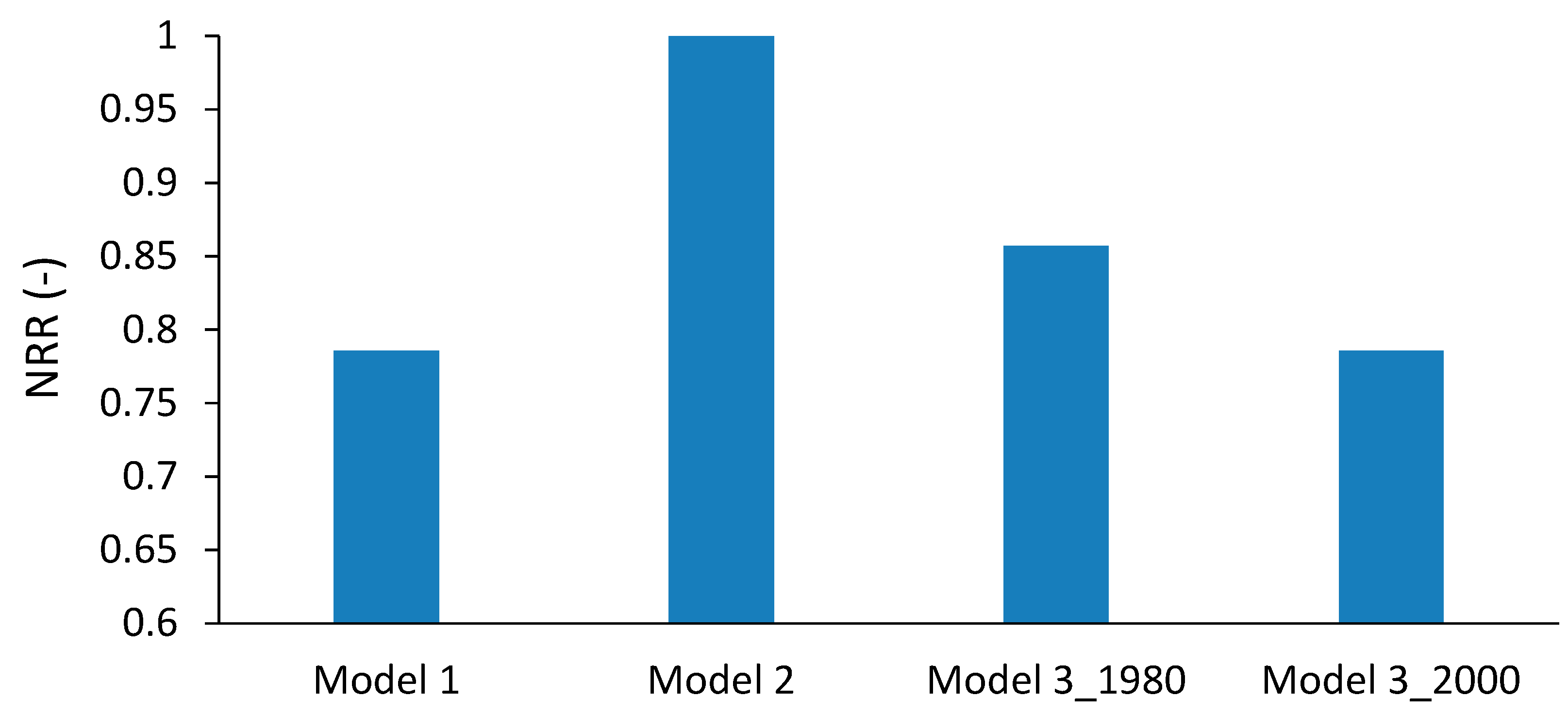
Overall, the histogram in Figure 10 summarizes the performances of all the adopted models in terms of No-Rejection Rate (NRR), defined as the ratio between the number of time series for which the hypothesis of model validity cannot be rejected, and the total number of analyzed time series. In many cases, it is sufficient to use Model 1 (NRR = 0.76, i.e., 11 out of 14 time series): this is mainly true if a rain gauge recorded a significant number of outlier events also in the last century.
Model 2 is able to reproduce all the time series inside the 95% CIs (NRR = 1), thus appearing as the preferable approach for a user, as it allows for only using information of rain gauge time series in the study area, without considering external sources.
Concerning the non-stationary approach, Model 3_2000 presents the same performance (NRR = 0.76) of the stationary Model 1. This is mainly due to the fact that some outliers of the last century (related to two out of three time series for which Model 1 has to be rejected: 1-day Vibo Valentia and 24-h Ardore Superiore data sets) are not inside the CIs of the stationary component (represented by dotted lines on the correspondent EV1 probabilistic plots). Moreover, for 1-h Vibo Valentia and 24-h Ardore Superiore data sets, the assumed period for trends appears insufficient to correctly reconstruct all the rainfall events occurred after 2000. A slight improvement is provided by Model 3_1980 (NRR = 0.86, i.e., 12 out of 14 time series). In this case, the assumed beginning of the trend allows to correctly reproduce 130.2 mm for 1-h Vibo Valentia time series, but the rejection for 1-day Vibo Valentia and 24-h Ardore Superiore data sets remains, due to the same reasons related to Model 3_2000.
Consequently, it does not seem essential to remove the hypothesis of stationary parameters, as significant trends do not appear from the observed data, due to a relevant number of heavy events which also occurred in the central part of the last century.
Furthermore, the described results in this work for annual maximum time series with daily and sub-daily durations confirm what is obtained in [17] concerning continuous daily series for the same investigated area, and thus they further highlight that rainfall data of Calabria do not show a clear increase in extreme events, in terms of intensity and frequency of occurrence, unlike other areas of the Mediterranean area, such as the Central Alps and Northern Italy [18,19].
Therefore, as also reported in [43], no general change can be asserted for the whole Mediterranean area; the findings of the analysis may depend on several local aspects, including the density of the rain gauge network as well.
The results of this work emphasize the importance of the observations of the past, in order to improve the knowledge of hydrological processes under investigation [14].
However, in this context there is a widespread perception that the past is no more representative of the future, and the statement ‘‘stationarity is dead’’ [44] is very popular in the hydrological community [45,46,47], although other scientists have criticized it [9,48,49,50]. The criticism, shared by the authors of this work, emerges from the fact that stationarity does not necessarily contradict the term “change” [9]. Very popular “examples” can be mentioned [9]: in the absence of an external force, the position of a body in motion changes in time but the velocity is unchanged (Newton’s first law); if a constant force is present, then the velocity changes but the acceleration is constant (Newton’s second law); if the force changes, e.g., the gravitational force with changing distance in planetary motion, the acceleration is no longer constant, but other invariant properties emerge, e.g., the angular momentum (Newton’s law of gravitation; see also [48]).
On the contrary, non-stationarity is usually considered as synonymous with change, but change is a general notion applicable everywhere, including to the real (material) world, while stationarity and non-stationarity are applied only to models, not to the real world [9].
4. Conclusions
The obtained results, regarding annual maximum rainfall series in the Calabria region, highlighted the importance of testing both stationary and non-stationary approaches, in order to better characterize time series of hydro-meteorological variables at daily and sub-daily scales.
In some cases it is sufficient to adopt the stationary model with constant parameters, in particular, when some outlier events occurred also in the last century. Moreover, a stationary approach with parameters as random variables allows the reconstruction of all the analyzed time series.
With the adopted parametric trends (assumed from external sources in order to not violate ergodicity), the non-stationary framework presents similar or slightly better performances with respect to a stationary model with deterministic parameters. These results are justified by two reasons: the stationary component of this framework does not correctly model some outlier events that occurred in the last century; the assumed period for trends could have an insufficient duration in order to reproduce the more recent events.
Consequently, if the hypothesis of a stationary process with parameters as random variables cannot be rejected, a user could surely prefer stationary frameworks. The obvious advantages are: the respect of ergodicity of the process (and then only the observed data series can be used); no other source of uncertainty is introduced, mainly related to the mathematical expression of the trends, the beginning , and the reliability of the external information (in particular, outputs from RCMs, characterized by a spatial resolution not compatible with rainfall phenomena at point-scale).
Overall, the obtained results in this work showed that, for annual maximum rainfall series in Calabria, it is not essential to remove the hypothesis of stationary parameters: significant trends do not appear from the observed data, as a relevant rate of heavy events also occurred in the central part of the last century. However, further analyses are needed, based on broader samples than annual maxima (for example POT—Peak Over Threshold series), in order to establish the more general validity of the results presented here. Obviously, these results do not imply any statement about climate changes (as discussed in Section 3), but they only intend to offer operating elements for an estimate of hydrological design extremes referred to a very close time window in the future.
The methodology, here applied, further suggests that a good modelling strategy should firstly consider the simplest approach, according to the principle of parsimony. In fact, using directly a more complex model instead of a simpler one could not be justified, without clear evidence from observed data, or understanding of physical dynamics.
Therefore, the stationary framework should represent the default assumption [49] and, even if there is evidence for non-stationarity, stationary models should be used as a benchmark for more complex approaches, in order to evaluate the magnitude of the improvements.
Lastly, uncertainty plays a crucial role in this context, related to model parameters (should a user assume them as deterministic or as random variables?), and to the other previously mentioned aspects referred to the use of a non-stationary model. Thus, adoption of few sources of uncertainty, or at most one (associated to the parameters assumed as random variables in a stationary framework), appears more competitive when changes of some features are not so clear from the data.
Author Contributions
Conceptualization, D.L.D.L. and L.G.; Data curation, D.L.D.L. and L.G.; Formal analysis, D.L.D.L.; Methodology, D.L.D.L. and L.G.; Software, D.L.D.L.; Supervision, D.L.D.L.; Validation, D.L.D.L.; Visualization, D.L.D.L.; Writing—original draft, D.L.D.L.and L.G.; Writing—review & editing, D.L.D.L.
Funding
This research received no external funding
Conflicts of Interest
The authors declare no conflict of interest.
Appendix A
In this appendix, the results of the frameworks’ application are shown for all the time series listed in Table 1 (except for 1-h and 1-day Vibo Valentia and 1-h and 24-h Ardore Superiore rainfall data, which were already discussed in Section 3).
Like in Section 3, for each time series the outcomes are represented in an EV1 probabilistic plot, related to Model 1, Model 2, Model 3_1980, and Model 3_2000, respectively.
Figure A1.
Chiaravalle Centrale rain gauge—annual maximum 1-h time series: application of (a) Model 1, (b) Model 2, (c) Model 3_1980 (the CIs of the stationary component are represented by dotted lines), (d) Model 3_2000 (the CIs of the stationary component are represented by dotted lines).
Figure A1.
Chiaravalle Centrale rain gauge—annual maximum 1-h time series: application of (a) Model 1, (b) Model 2, (c) Model 3_1980 (the CIs of the stationary component are represented by dotted lines), (d) Model 3_2000 (the CIs of the stationary component are represented by dotted lines).

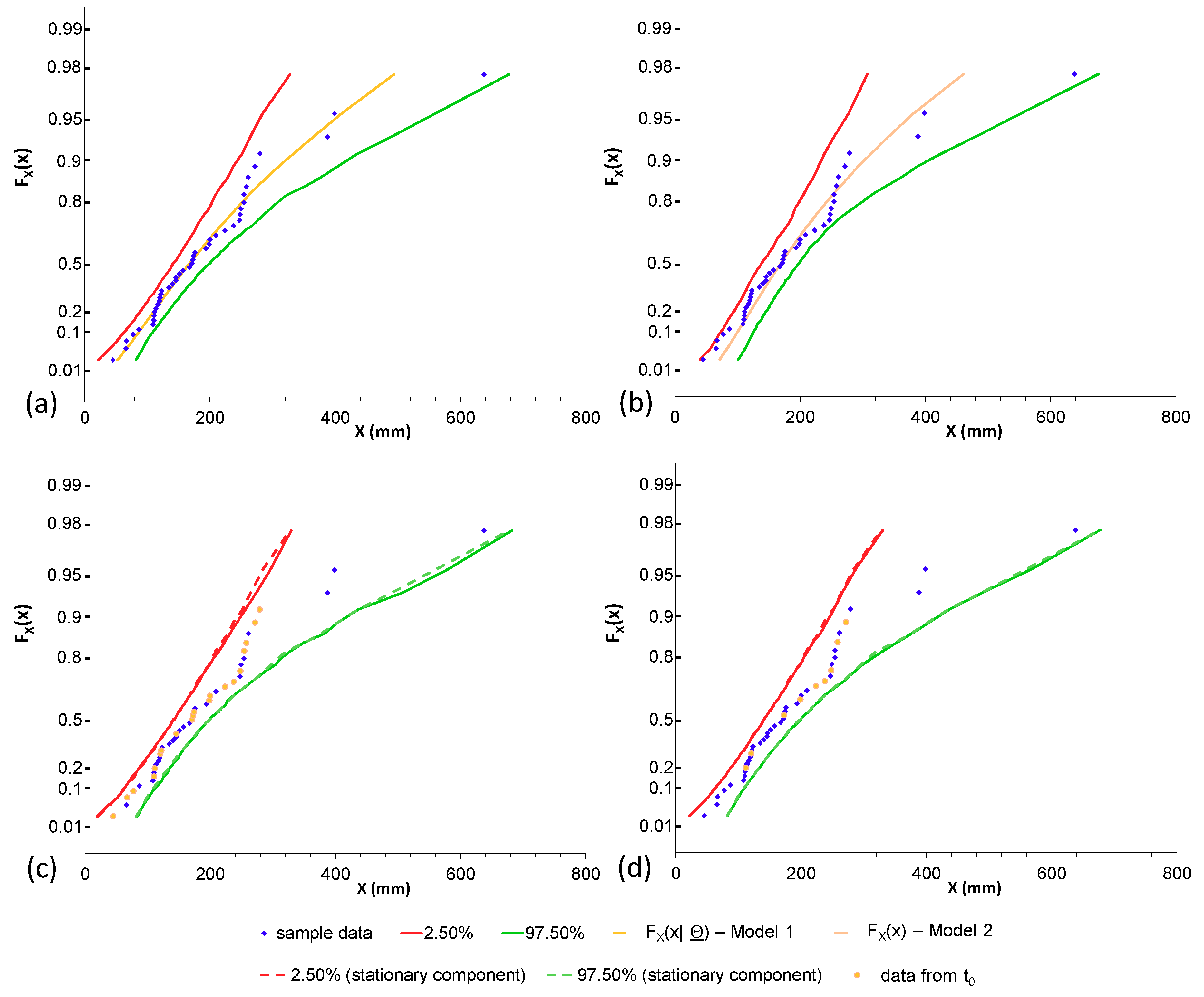
Figure A2.
Chiaravalle Centrale rain gauge—annual maximum 24-h time series: application of (a) Model 1, (b) Model 2, (c) Model 3_1980 (the CIs of the stationary component are represented by dotted lines), (d) Model 3_2000 (the CIs of the stationary component are represented by dotted lines).
Figure A2.
Chiaravalle Centrale rain gauge—annual maximum 24-h time series: application of (a) Model 1, (b) Model 2, (c) Model 3_1980 (the CIs of the stationary component are represented by dotted lines), (d) Model 3_2000 (the CIs of the stationary component are represented by dotted lines).


Figure A3.
Santa Cristina d’Aspromonte rain gauge—annual maximum 24-h time series: application of (a) Model 1, (b) Model 2, (c) Model 3_1980 (the CIs of the stationary component are represented by dotted lines), (d) Model 3_2000 (the CIs of the stationary component are represented by dotted lines).
Figure A3.
Santa Cristina d’Aspromonte rain gauge—annual maximum 24-h time series: application of (a) Model 1, (b) Model 2, (c) Model 3_1980 (the CIs of the stationary component are represented by dotted lines), (d) Model 3_2000 (the CIs of the stationary component are represented by dotted lines).

Figure A4.
Montalto Uffugo rain gauge—annual maximum 24-h time series: application of (a) Model 1, (b) Model 2, (c) Model 3_1980 (the CIs of the stationary component are represented by dotted lines), (d) Model 3_2000 (the CIs of the stationary component are represented by dotted lines).
Figure A4.
Montalto Uffugo rain gauge—annual maximum 24-h time series: application of (a) Model 1, (b) Model 2, (c) Model 3_1980 (the CIs of the stationary component are represented by dotted lines), (d) Model 3_2000 (the CIs of the stationary component are represented by dotted lines).

Figure A5.
Sant’Agata del Bianco rain gauge—annual maximum 1-day time series: application of (a) Model 1, (b) Model 2, (c) Model 3_1980 (the CIs of the stationary component are represented by dotted lines), (d) Model 3_2000 (the CIs of the stationary component are represented by dotted lines).
Figure A5.
Sant’Agata del Bianco rain gauge—annual maximum 1-day time series: application of (a) Model 1, (b) Model 2, (c) Model 3_1980 (the CIs of the stationary component are represented by dotted lines), (d) Model 3_2000 (the CIs of the stationary component are represented by dotted lines).


Figure A6.
Gioiosa Ionica rain gauge—annual maximum 3-h time series: application of (a) Model 1, (b) Model 2, (c) Model 3_1980 (the CIs of the stationary component are represented by dotted lines), (d) Model 3_2000 (the CIs of the stationary component are represented by dotted lines).
Figure A6.
Gioiosa Ionica rain gauge—annual maximum 3-h time series: application of (a) Model 1, (b) Model 2, (c) Model 3_1980 (the CIs of the stationary component are represented by dotted lines), (d) Model 3_2000 (the CIs of the stationary component are represented by dotted lines).

Figure A7.
Platì rain gauge—annual maximum 24-h time series: application of (a) Model 1, (b) Model 2, (c) Model 3_1980 (the CIs of the stationary component are represented by dotted lines), (d) Model 3_2000 (the CIs of the stationary component are represented by dotted lines).
Figure A7.
Platì rain gauge—annual maximum 24-h time series: application of (a) Model 1, (b) Model 2, (c) Model 3_1980 (the CIs of the stationary component are represented by dotted lines), (d) Model 3_2000 (the CIs of the stationary component are represented by dotted lines).

Figure A8.
Serra San Bruno rain gauge—annual maximum 1-h time series: application of (a) Model 1, (b) Model 2, (c) Model 3_1980 (the CIs of the stationary component are represented by dotted lines), (d) Model 3_2000 (the CIs of the stationary component are represented by dotted lines).
Figure A8.
Serra San Bruno rain gauge—annual maximum 1-h time series: application of (a) Model 1, (b) Model 2, (c) Model 3_1980 (the CIs of the stationary component are represented by dotted lines), (d) Model 3_2000 (the CIs of the stationary component are represented by dotted lines).


Figure A9.
Albi rain gauge—annual maximum 3-h time series: application of (a) Model 1, (b) Model 2, (c) Model 3_1980 (the CIs of the stationary component are represented by dotted lines), (d) Model 3_2000 (the CIs of the stationary component are represented by dotted lines).
Figure A9.
Albi rain gauge—annual maximum 3-h time series: application of (a) Model 1, (b) Model 2, (c) Model 3_1980 (the CIs of the stationary component are represented by dotted lines), (d) Model 3_2000 (the CIs of the stationary component are represented by dotted lines).

Figure A10.
Cittanova rain gauge—nnual maximum 6-h time series: application of (a) Model 1, (b) Model 2, (c) Model 3_1980 (the CIs of the stationary component are represented by dotted lines), (d) Model 3_2000 (the CIs of the stationary component are represented by dotted lines).
Figure A10.
Cittanova rain gauge—nnual maximum 6-h time series: application of (a) Model 1, (b) Model 2, (c) Model 3_1980 (the CIs of the stationary component are represented by dotted lines), (d) Model 3_2000 (the CIs of the stationary component are represented by dotted lines).

References
- Chow, V.T.; Maidment, D.R.; Mays, L.W. Applied Hydrology, 2nd ed.; McGraw-Hill: New York, NY, USA, 2013; pp. 1–624. ISBN 9780071743914. [Google Scholar]
- Serinaldi, F.; Kilsby, C.G. Stationarity is undead: Uncertainty dominates the distribution of extremes. Adv. Water Resour. 2015, 77, 17–36. [Google Scholar] [CrossRef]
- Serinaldi, F. An uncertain journey around the tails of multivariate hydrological distributions. Water Resour. Res. 2013, 49, 6527–6547. [Google Scholar] [CrossRef] [Green Version]
- Serinaldi, F. Assessing the applicability of fractional order statistics for computing confidence intervals for extreme quantiles. J. Hydrol. 2009, 376, 528–541. [Google Scholar] [CrossRef]
- Salas, J.D.; Obeysekera, J. Revisiting the Concepts of Return Period and Risk for Nonstationary Hydrologic Extreme Events. J. Hydrol. Eng. 2014, 19, 554–568. [Google Scholar] [CrossRef]
- Acero, F.J.; Parey, S.; García, J.A.; Dacunha-Castelle, D. Return Level Estimation of Extreme Rainfall over the Iberian Peninsula: Comparison of Methods. Water 2018, 10, 179. [Google Scholar] [CrossRef]
- Cheng, L.; AghaKouchak, A.; Gilleland, E.; Katz, R.W. Non-stationary extreme value analysis in a changing climate. Clim. Chang. 2014, 127, 353–369. [Google Scholar] [CrossRef]
- Rootzén, H.; Katz, R.W. Design life level: Quantifying risk in a changing climate. Water Resour. Res. 2013, 49, 5964–5972. [Google Scholar] [CrossRef]
- Koutsoyiannis, D.; Montanari, A. Negligent killing of scientific concepts: The stationarity case. Hydrol. Sci. J. 2014, 60, 1174–1183. [Google Scholar] [CrossRef]
- Klemeš, V. Tall tales about tails of hydrological distributions. J. Hydrol. Eng. 2000, 5, 227–231. [Google Scholar] [CrossRef]
- Gabriele, S.; Arnell, N. A hierarchical approach to regional flood frequency analysis. Water Resour. Res. 1991, 27, 1281–1289. [Google Scholar] [CrossRef]
- Obeysekera, J.; Salas, J.D. Quantifying the uncertainty of design floods under nonstationary conditions. J. Hydrol. Eng. 2014, 19, 1438–1446. [Google Scholar] [CrossRef]
- Stedinger, J.R.; Griffis, V.W. Getting from here to where? Flood frequency analysis and climate. J. Am. Water Resour. Assoc. 2011, 47, 506–513. [Google Scholar] [CrossRef]
- Montanari, A.; Koutsoyiannis, D. Modeling and mitigating natural hazards: Stationarity is immortal! Water Resour. Res. 2014, 50, 9748–9756. [Google Scholar] [CrossRef] [Green Version]
- Biondi, D.; De Luca, D.L. Rainfall-runoff model parameter conditioning on regional hydrological signatures: Application to ungauged basins in southern Italy. Hydrol. Res. 2017, 48, 714–725. [Google Scholar] [CrossRef]
- Laio, F.; Di Baldassarre, G.; Montanari, A. Model selection techniques for the frequency analysis of hydrological extremes. Water Resour. Res. 2009, 45, W07416. [Google Scholar] [CrossRef]
- Caloiero, T.; Coscarelli, R.; Ferrari, E.; Sirangelo, B. Trends in the daily precipitation categories of Calabria (southern Italy). Procedia Eng. 2016, 162, 32–38. [Google Scholar] [CrossRef]
- Brunetti, M.; Maugeri, M.; Nanni, T. Changes in total precipitation, rainy days and extreme events in northeastern Italy. Int. J. Climatol. 2001, 21, 861–871. [Google Scholar] [CrossRef] [Green Version]
- Brugnara, Y.; Brunetti, M.; Maugeri, M.; Nanni, T.; Simolo, C. High-resolution analysis of daily precipitation trends in the central Alps over the last century. Int. J. Climatol. 2012, 32, 1406–1422. [Google Scholar] [CrossRef]
- Rodrigo, F.S.; Trigo, R.M. Trends in daily rainfall in the Iberian Peninsula from 1951 to 2002. Int. J. Climatol. 2007, 27, 513–529. [Google Scholar] [CrossRef] [Green Version]
- Alpert, P.; Ben-Gai, T.; Baharad, A.; Benjamini, Y.; Yekutieli, D.; Colacino, M.; Diodato, L.; Ramis, C.; Homar, V.; Romero, R.; et al. The paradoxical increase of Mediterranean extreme daily rainfall in spite of decrease in total values. Geophys. Res. Lett. 2002, 29, 1–31. [Google Scholar] [CrossRef]
- Rossi, F.; Fiorentino, M.; Versace, P. Two-component extreme value distribution for flood frequency analysis. Water Resour. Res. 1984, 20, 847–856. [Google Scholar]
- Buttafuoco, G.; Caloiero, T.; Coscarelli, R. Spatial and temporal patterns of the mean annual precipitation at decadal time scale in southern Italy (Calabria region). Theor. Appl. Climatol. 2011, 105, 431–444. [Google Scholar] [CrossRef]
- Federico, S.; Avolio, E.; Pasqualoni, L.; Bellecci, C. Atmospheric patterns for heavy rain events in Calabria. Nat. Hazards Earth Syst. Sci. 2008, 8, 1173–1186. [Google Scholar] [CrossRef] [Green Version]
- Dubey, S.D. Compound gamma, beta and F distributions. Metrika 1970, 16, 27–31. [Google Scholar] [CrossRef]
- Koutsoyiannis, D. Statistics of extremes and estimation of extreme rainfall. I: Theoretical investigation. Hydrol. Sci. J. 2004, 49, 575–590. [Google Scholar] [CrossRef]
- Van Montfort, M.A.J.; van Putten, B. A comment on modelling extremes: Links between multi-component extreme value and general extreme value distributions. J. Hydrol. N. Z. 2002, 41, 197–202. [Google Scholar]
- Dalrymple, T. Flood-frequency analyses, Manual of Hydrology: Part 3. Water Supply Pap. 1960, 1543A. [Google Scholar] [CrossRef]
- Abramowitz, M.; Stegun, I.A. Handbook of Mathematical Functions with Formulas, Graphs, Mathematical Tables, 10th ed.; Dover Publications, Inc.: Mineola, NY, USA, 1972. [Google Scholar]
- Beran, M.A.; Hosking, J.R.M.; Arnell, N.W. Comment on ‘Two-component extreme value distribution for flood frequency analysis,’ by Fabio Rossi, Mauro Fiorentino, and Pasquale Versace. Water Resour. Res. 1986, 22, 263–266. [Google Scholar] [CrossRef]
- Versace, P.; Ferrari, E.; Gabriele, S.; Rossi, F. Valutazione delle Piene in Calabria; CNR-IRPI e GNDCI: Geodata, Cosenza, Italy, 1989. (In Italian) [Google Scholar]
- Arnell, N.; Gabriele, S. The performance of the Two Component Extreme Value distribution in regional flood frequency analysis. Water Resour. Res. 1988, 24, 879–887. [Google Scholar] [CrossRef]
- Fiorentino, M.K.; Arora, K.; Singh, V.P. The two-component extreme value distribution for flood frequency analysis: Derivation of a new estimation method. Stoch. Hydrol. Hydraul. 1987, 1, 199–208. [Google Scholar] [CrossRef]
- Biondi, D.; Cruscomagno, F.; De Luca, D.L.; Ferrari, E.; Versace, P. La valutazione delle piene in Calabria: 1989–2013 (in Italian). In Proceedings of the XXXIV Corso di Aggiornamento Tecniche per la Difesa dall’Inquinamento, Guardia Piemontese, CS, Italy, 19–22 June 2013; pp. 187–216. [Google Scholar]
- Kottegoda, N.T.; Rosso, R. Applied Statistics for Civil and Environmental Engineers; Wiley-Blackwell: Hoboken, NJ, USA, 2008; p. 736. ISBN 978-1-405-17917-1. [Google Scholar]
- EEA—European Environment Agency. Climate Change Adaptation ad Disaster Risk Reduction in Europe; EEA: Kongens Nytorv, Denmark, 2017; Volume 15, pp. 1–171. [Google Scholar]
- ISPRA—Istituto Superiore per la Protezione e la Ricerca Ambientale. Il Clima Futuro in Italia: Analisi delle proiezioni dei modelli regionali; ISPRA: Via Vitaliano Brancati, Roma, 2015; Volume 58, pp. 1–64. ISBN 978-88-448-0723-8. (In Italian) [Google Scholar]
- Ban, N.; Schmidli, J.; Schär, C. Heavy precipitation in a changing climate: Does short-term summer precipitation increase faster? Geophys Res. Lett. 2015, 42, 1165–1172. [Google Scholar] [CrossRef] [Green Version]
- Chan, S.C.; Kendon, E.J.; Fowler, H.J.; Blenkinsop, S.; Roberts, N.M.; Ferro, C.A.T. The value of high-resolution Met Office regional climate models in the simulation of multihourly precipitation extremes. J. Clim. 2014, 27, 6155–6174. [Google Scholar] [CrossRef]
- Kendon, E.J.; Roberts, N.M.; Fowler, H.J.; Roberts, M.J.; Chan, S.C.; Senior, C.A. Heavier summer downpours with climate change revealed by weather forecast resolution model. Nat. Clim. Chang. 2014, 4, 570–576. [Google Scholar] [CrossRef]
- Lehmann, J.; Coumou, D.; Frieler, K. Increased record-breaking precipitation events under global warming. Clim. Chang. 2015, 132, 501–515. [Google Scholar] [CrossRef]
- Weibull, W. A statistical theory of strength of materials. Ing. Vetensk. Akad. Handl. 1939, 151, 1–45. [Google Scholar]
- Reiser, H.; Kutiel, H. Rainfall uncertainty in the Mediterranean: Time series, uncertainty, and extremes. Theor. Appl. Climatol. 2011, 104, 357–375. [Google Scholar] [CrossRef]
- Milly, P.C.D.; Betancourt, J.; Falkenmark, M.; Hirsch, R.M.; Kundzewicz, Z.W.; Lettenmaier, D.P.; Stouffer, R.J. Stationarity is dead: Whither water management? Science 2008, 319, 573–574. [Google Scholar] [CrossRef] [PubMed]
- Purkey, D.R.; Escobar Arias, M.I.; Mehta, V.K.; Forni, L.; Depsky, N.J.; Yates, D.N.; Stevenson, W.N. A philosophical justification for a novel analysis-supported, stakeholder-driven participatory process for water resources planning and decision making. Water 2018, 10, 1009. [Google Scholar] [CrossRef]
- Yunbiao, W.; Lianqing, X. Nonstationary modelling of annual discharge over the Tarim River headstream catchment, China. IOP Conf. Ser. Earth Environ. Sci. 2018, 170, 022149. [Google Scholar] [CrossRef]
- Zhang, T.; Wang, Y.; Wang, B.; Tan, S.; Feng, P. Nonstationary flood frequency analysis using univariate and bivariate time-varying models based on GAMLSS. Water 2018, 10, 819. [Google Scholar] [CrossRef]
- Koutsoyiannis, D. Hurst-Kolmogorov dynamics and uncertainty. J. Am. Water Resour. Assoc. 2011, 47, 481–495. [Google Scholar] [CrossRef]
- Lins, H.F.; Cohn, T.A. Stationarity: Wanted dead or alive? J. Am. Water Resour. Assoc. 2011, 47, 475–480. [Google Scholar] [CrossRef]
- Matalas, N.C. Comment on the announced death of stationarity. J. Water Resour. Plan. Manag. 2012, 138, 311–312. [Google Scholar] [CrossRef]
Figure 1.
Study area of the Calabria region (southern Italy): rain gauge network (blue points), rain gauges considered in this work (red points with ID code labelled), sub-regions Tyrrhenian (green polygons), Central (yellow polygon), and Ionian (pink polygons).
Figure 1.
Study area of the Calabria region (southern Italy): rain gauge network (blue points), rain gauges considered in this work (red points with ID code labelled), sub-regions Tyrrhenian (green polygons), Central (yellow polygon), and Ionian (pink polygons).

Figure 2.
Frequency distributions of on normal probability plot, for N = 40 (orange points), N = 80 (red points), N = 500 (blue points).
Figure 2.
Frequency distributions of on normal probability plot, for N = 40 (orange points), N = 80 (red points), N = 500 (blue points).

Figure 3.
Frequency distributions of on log-normal probability plot, for N = 40 (orange points), N = 80 (red points), N = 500 (blue points).
Figure 3.
Frequency distributions of on log-normal probability plot, for N = 40 (orange points), N = 80 (red points), N = 500 (blue points).

Figure 4.
Dependence of standard deviations and on sample size N.

Figure 5.
Dispersion plot with all the values and .

Figure 6.
Vibo Valentia rain gauge—annual maximum 1-h time series: application of (a) Model 1, (b) Model 2, (c) Model 3_1980 (the CIs of the stationary component are represented by dotted lines), (d) Model 3_2000 (the CIs of the stationary component are represented by dotted lines).
Figure 6.
Vibo Valentia rain gauge—annual maximum 1-h time series: application of (a) Model 1, (b) Model 2, (c) Model 3_1980 (the CIs of the stationary component are represented by dotted lines), (d) Model 3_2000 (the CIs of the stationary component are represented by dotted lines).

Figure 7.
Vibo Valentia rain gauge—annual maximum 1-day time series: application of (a) Model 1, (b) Model 2, (c) Model 3_1980 (the CIs of the stationary component are represented by dotted lines), (d) Model 3_2000 (the CIs of the stationary component are represented by dotted lines).
Figure 7.
Vibo Valentia rain gauge—annual maximum 1-day time series: application of (a) Model 1, (b) Model 2, (c) Model 3_1980 (the CIs of the stationary component are represented by dotted lines), (d) Model 3_2000 (the CIs of the stationary component are represented by dotted lines).

Figure 8.
Ardore Superiore rain gauge—annual maximum 1-h time series: application of (a) Model 1, (b) Model 2, (c) Model 3_1980 (the CIs of the stationary component are represented by dotted lines), (d) Model 3_2000 (the CIs of the stationary component are represented by dotted lines).
Figure 8.
Ardore Superiore rain gauge—annual maximum 1-h time series: application of (a) Model 1, (b) Model 2, (c) Model 3_1980 (the CIs of the stationary component are represented by dotted lines), (d) Model 3_2000 (the CIs of the stationary component are represented by dotted lines).

Figure 9.
Ardore Superiore rain gauge—annual maximum 24-h time series: application of (a) Model 1, (b) Model 2, (c) Model 3_1980 (the CIs of the stationary component are represented by dotted lines), (d) Model 3_2000 (the CIs of the stationary component are represented by dotted lines).
Figure 9.
Ardore Superiore rain gauge—annual maximum 24-h time series: application of (a) Model 1, (b) Model 2, (c) Model 3_1980 (the CIs of the stationary component are represented by dotted lines), (d) Model 3_2000 (the CIs of the stationary component are represented by dotted lines).

Figure 10.
Histogram of No-Rejection Rate (NRR) for each adopted model.


Table 1.
List and characteristics of analyzed time series in this work.
| Rain Gauge | MAP (mm) | Duration | N (-) | Elevation (m a.s.l.) | Heavy Rainfall Events from 1 January 2000 (mm) | Heavy Rainfall Events before 1 January 2000 (mm) |
|---|---|---|---|---|---|---|
| Vibo Valentia (ID code 2800) | 951.1 | 1 h | 61 | 498 | 130.2 (3 July 2006) | |
| 1 day | 94 | 202.6 (3 July 2006) | 325.1 (2 December 1938) | |||
| Chiaravalle Centrale (ID code 1960) | 1439.7 | 1 h | 67 | 714 | 84.2 (10 September 2000) | |
| 114.8 (25 September 2009) | ||||||
| 24 h | 70 | 359.6 (9 September 2000) | 416 (25 November 1993) 512 (16 October 1951) 432.4 (21 November 1935) | |||
| 373.2 (31 October 2015) | ||||||
| Santa Cristina d’Aspromonte (ID code 2540) | 1500.9 | 24 h | 44 | 510 | 271.6 (31 October 2015) | 279.2 (3 October 1996) |
| 398.7 (23 November 1959) | ||||||
| 637.9 (16 October 1951) | ||||||
| 388.1 (22 January 1946) | ||||||
| Ardore Superiore (ID code 2210) | 928.7 | 1 h | 53 | 250 | 118.4 (30 September 2000) | |
| 98.6 (25–26 November 2016) | ||||||
| 24 h | 56 | 430.2 (29 September 2000) | 321.3 (17 October 1951) 325.6 (5 December 1933) | |||
| 321.4 (1 November 2015) | ||||||
| 362.4 (25–26 November 2016) | ||||||
| Montalto Uffugo (ID code 1060) | 1393.7 | 24 h | 61 | 468 | 224.8 (12 December 2008) | |
| Sant’Agata del Bianco (ID code 2270) | 1059.2 | 1 day | 86 | 380 | 370.4 (1 November 2015) 393 (25 November 2016) | |
| Gioiosa Ionica (ID code 2160) | 899.1 | 3 h | 62 | 125 | 122.8 (25 November 2016) | 108.8 (22 September 1965) |
| 101.7 (3 November 1953) | ||||||
| 114.1 (17 October 1951) | ||||||
| 111.3 (21 November 1935) | ||||||
| 105.1 (10 November 1932) | ||||||
| Platì (ID code 2230) | 1775.9 | 24 h | 45 | 310 | 332 (1 November 2015) | 286.3 (21 October 1953) |
| Serra San Bruno (ID code 1980) | 1779.7 | 1 h | 71 | 790 | 100.4 (19 November 2013) | 95.4 (12 September 1958) |
| 90 (22 November 1935) | ||||||
| Albi (ID code 1830) | 1251.1 | 3 h | 57 | 710 | 172.8 (19 November 2013) | 127.7 (9 September 1939) |
| 109.3 (21 October 1935) | ||||||
| Cittanova (ID code 2600) | 1463.7 | 6 h | 70 | 407 | 307.4 (22 November 2011) | 185.1 (18 October 1951) |
Table 2.
Two-Component Extreme Value (TCEV) distribution of rainfall annual maxima with daily and sub-daily durations: regional values of , , and for the Calabria region [34].
Table 2.
Two-Component Extreme Value (TCEV) distribution of rainfall annual maxima with daily and sub-daily durations: regional values of , , and for the Calabria region [34].
| Parameter | Value | Regional Level |
|---|---|---|
| 0.449 | 1st (the whole Calabria region) | |
| 2.168 | ||
| 36 | 2nd (Tyrrhenian sub-region ) | |
| 16.7 | 2nd (Central sub-region) | |
| 10.3 | 2nd (Ionian sub-region) |
© 2018 by the authors. Licensee MDPI, Basel, Switzerland. This article is an open access article distributed under the terms and conditions of the Creative Commons Attribution (CC BY) license (http://creativecommons.org/licenses/by/4.0/).
Share and Cite
MDPI and ACS Style
De Luca, D.L.; Galasso, L. Stationary and Non-Stationary Frameworks for Extreme Rainfall Time Series in Southern Italy. Water 2018, 10, 1477. https://doi.org/10.3390/w10101477
AMA Style
De Luca DL, Galasso L. Stationary and Non-Stationary Frameworks for Extreme Rainfall Time Series in Southern Italy. Water. 2018; 10(10):1477. https://doi.org/10.3390/w10101477
Chicago/Turabian StyleDe Luca, Davide Luciano, and Luciano Galasso. 2018. "Stationary and Non-Stationary Frameworks for Extreme Rainfall Time Series in Southern Italy" Water 10, no. 10: 1477. https://doi.org/10.3390/w10101477
Note that from the first issue of 2016, this journal uses article numbers instead of page numbers. See further details here.