A Theoretically Derived Probability Distribution of Scour


1
Department of European and Mediterranean Cultures, University of Basilicata, 75100 Matera, Italy
2
Department of Civil Engineering, Universidad de Concepción, Concepción 4030000, Chile
*
Author to whom correspondence should be addressed.
Water 2018, 10(11), 1520; https://doi.org/10.3390/w10111520
Submission received: 11 September 2018
/
Revised: 20 October 2018
/
Accepted: 21 October 2018
/
Published: 26 October 2018
(This article belongs to the Section Hydraulics and Hydrodynamics)
Abstract
:Based on recent contributions regarding the treatment of unsteady hydraulic conditions in the state-of-the-art scour literature, theoretically derived probability distribution of bridge scour is introduced. The model has been derived assuming a rectangular hydrograph shape with a given duration, and a random flood peak, following a Gumbel distribution. A model extension for a more complex flood event has also been presented, assuming a synthetic exponential hydrograph shape. The mathematical formulation can be extended to any flood-peak probability distribution. The aim of the paper is to move forward the current approaches adopted for the bridge design, by coupling hydrological, hydraulic, and erosional models, in a mathematical closed form. An example of the application of the proposed distribution has been included with the aim to provide a guidance for the parameters estimation.

1. Introduction
The scour process is one of the major causes of bridge collapse, on a global scale. It is responsible for more than 50% of bridge failures, according to recent studies by Proske [1]. Therefore, understanding the complex interactions between river systems and bridges is critical to advance our ability to prevent such catastrophic events and protect our infrastructures.
It is interesting to mention that the actual bridge design manuals recommend the use of the maximum equilibrium scour depth to withstand erosional forces due to extreme flood events (see [2,3]). Therefore, most modern bridges have been designed under such hypotheses, assuming a flood peak discharge with a return period of 100–200 years. This should lead to good safety conditions, but scour-induced bridge failures occur under considerably scattered flood peak events, with a range of return periods ranging from one to more than 1000 years [4]. This clearly highlights some gaps in our understanding of the overall dynamics and inadequacy of existing regulations.
Such uncertainty on the safety conditions of river bridges may be partly due to the scale effects involved in estimations of real-life scour using scour formulas derived from laboratory experiments with idealized hydraulic, sedimentological, and geometrical conditions [5]. Unfortunately, the up-scale of laboratory models to field case studies is still far from realization, given the complete lack of reliable field scour data. In fact, bridge-scour field monitoring implies a number of technical issues (e.g., turbid currents, sensor damage) that have limited the development of a dedicated technology.
Nevertheless, scientific literature offers a wide spectrum of applications that provide a well-defined formalism to characterize the maximum equilibrium scour depth achieved under clear-water and steady hydraulic conditions [6,7]. However, extreme flood events lead to a more complex mechanisms, such as the interaction among unsteady hydraulic conditions, short- and long-term riverbed evolution, and refilling of the scour-hole [8,9].
The lack of more realistic hydraulic conditions in laboratory-based scour experiments is attributed to experimental difficulties associated with discharging control in flumes and to hydraulic pump volume capacity and sediment recirculation systems. Only recently, time-dependent scour formulas, without considering a step-hydrograph have been introduced (e.g., [10,11,12,13]). Among others, Link et al. [12] and Pizarro et al. [14] introduced the concept of dimensionless effective flow work () that has shown good predictive capabilities under several experimental conditions, both in steady and non-steady conditions. The introduction of the flow work parameter has stimulated a number of subsequent studies that have further explored this index to derive a time-dependent scour formulation (e.g., [13]). Such a mathematical formulation offers the opportunity to export recent results on the scour process into the field of probability, searching for potential links between flood statistics and scour. This may help overcome some of the existing limitations in the river bridge design.
This paper aims to investigate the theoretically derived probability distribution of the bridge scour process, with the aim of motivating and moving forward the current approaches adopted for the hydraulic design of bridges. Hydrological, hydraulic, and scour models are coupled in a mathematical closed form. The article is organized as follows: Hydraulic assumptions are presented in Section 2 and Section 3 describes the mathematical derivation of the theoretical probability distribution of scour. Conclusions are presented at the end.
2. Hydraulic Assumptions
Interactions between river flow and bridges must be delineated, adopting a number of simplifying assumptions able to capture the main dynamics occurring in a river. In particular, river flow discharge () can be expressed as the product of two factors, namely mean flow velocity () and the associated wetted area of the cross section ():
Following Manfreda [15], it is possible to write both terms as a function of the hydraulic water stage (),
and therefore, the combination of Equations (2) and (3) allows expression of the flow discharge as a function of the mean flow velocity:
Inverting Equation (4) makes it possible to derive as a function of ,
where , and .
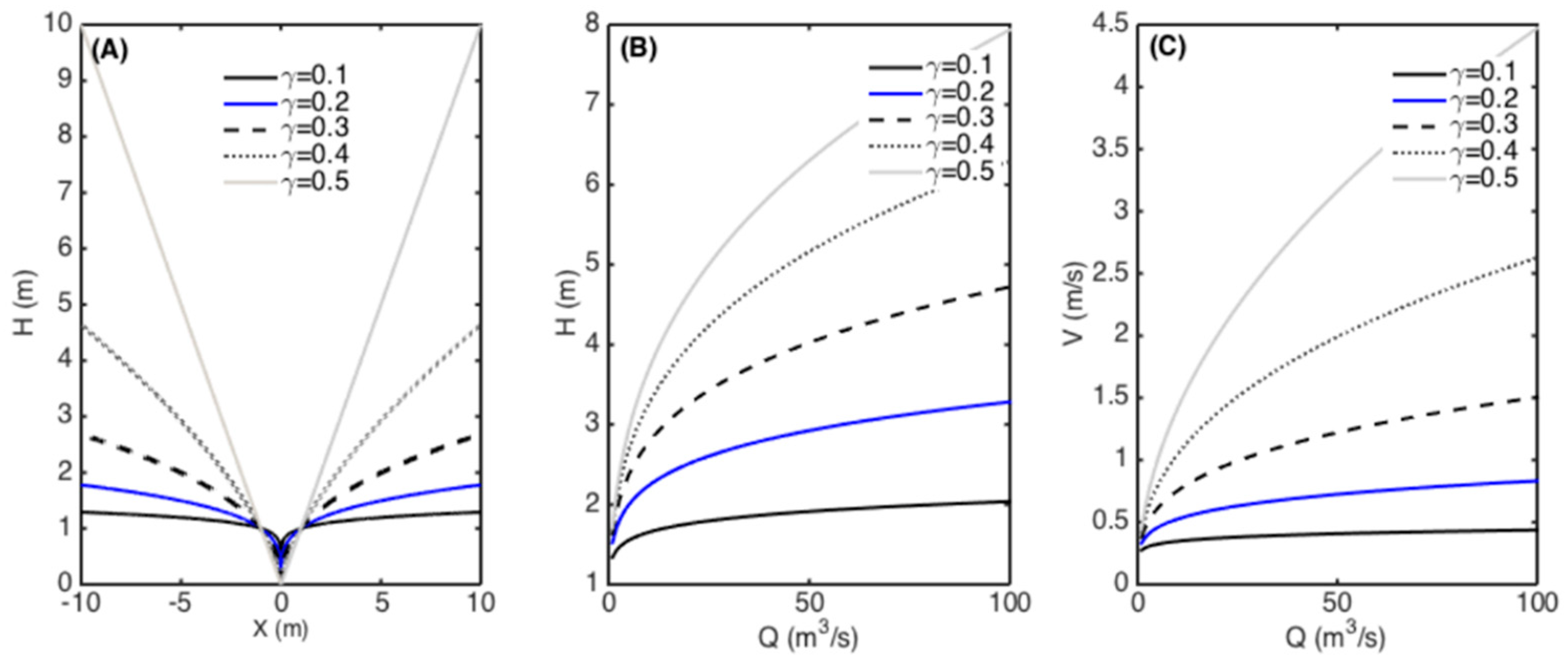
This formalism allows the description of the mathematical relationship between the mean flow velocity and the discharge, in a given cross-section. An example is given in Figure 1, where different cross-sections are plotted together with the corresponding flow rating curve (H(Q)) (panel B) and the velocity as a function of the discharge (panel C). These examples are derived numerically with the aim of better explaining the role played by the parameter , which controls the shape of the cross-section and consequently its hydraulic behavior. The numerical examples are derived by assuming symmetric cross-sections with side-slopes described by a parabolic function. Side slopes are steeper with the increase of the parameter producing marked differences in the corresponding flow rating curves.
Considering that the probability distribution of the flow-peak discharge is a well-described process in hydrology, it is possible to exploit this knowledge to derive the probability distribution of mean flow velocity and consequently of the scour. The details of such an idea are better addressed in the following section.
3. The Theoretically Derived Distribution of Scour (TDDS)
3.1. Simplified Rectangular Flood Hydrograph
A simplified hydrograph shape (with constant discharge and duration ) is assumed to derive the probability distribution of scour. This leads to a mathematical description of the dynamic of the scour process over their entire possible range of flood frequencies.
On one hand, the probability distribution of floods is well known and parameters of flood distribution can be calibrated using local or regional approaches [16,17,18,19,20,21]. In the present case, it starts from the hypothesis of a Gumbel distribution,
where is the probability distribution of floods, and and are Gumbel parameters.
On the other hand, the relationship between a given flood event and the produced scour can be interpreted by different methods. The authors had recently proposed the dimensionless effective flow work () which is computed as a function of the flow velocity, , [14]:
where is the critical velocity for the incipient scour, is a reference velocity, is a reference time, is the pier-diameter, is the sediment grain-size, is the relative density with subscripts and referring to sediment and water, respectively, is the gravitational acceleration, and is a reference length.
The variable gives the great advantage of properly interpreting the scour process in time, under any flood hydrograph. Moreover, this formulation allows to link the scour process to the flood through the mean flow velocity term. It is true that does not necessarily properly represent local dynamics around bridge foundations, but it is a necessary approximation to build a probabilistic model of scour.
Assuming a rectangular hydrograph allows the solution of the integral of Equation (7), providing a simple expression of the total flow work, associated with a given flood event, with a certain magnitude and duration that can be used for the subsequent steps. It is possible to assume a more complex hydrograph shape, but this makes the mathematical tractability of the function more complex. Therefore, the authors decided to keep the model as simple as possible to identify an analytical solution for the probability distribution of scour. Nevertheless, additional complexity can be introduced in the presented modeling scheme, by means of a numerical integration, in the subsequent steps.
Inverting Equation (7), it is possible to obtain an expression of as a function of for a rectangular hydrograph,
Furthermore, given , the scour depth can be estimated using the bridge–pier scour entropic (BRISENT) model recently introduced by Pizarro et al. [13]:
where is the normalized scour depth, is the scour depth, is the entropic-scour parameter, is a fitting coefficient, and is the maximum relative scour depth associated with the maximum dimensionless, effective flow work, . Inverting Equation (9), it is possible to express as a function of ,
Consequently, the mathematical relation between and can be written as,
where .
Using Equation (11), we can derive the probability distribution of scour, , based on the probability distribution of floods (Equation (6)). The mathematical formulation becomes:
Note that Equation (12) is a function defined between 0 and , and therefore it has two mass probabilities, at these scour depths. Consequently, to properly describe the distribution, it is necessary to estimate the probability that the scour depth is equal to zero for all the possible realizations of floods. This value can be estimated by integrating the derived probability distribution of mean flow velocities ,
The probability of zero scour can be thus defined as:
However, there might also be a mass probability for the value that might be computed as:
The proposed formulations describe the statistics of the dimensionless scour commonly used in all laboratory studies. Nevertheless, it is straightforward to obtain the expressions referred to the dimensional scour z, using the reference length, , described in Equation (7). In particular, the dimensional scour z = and the probability density function becomes:
while the probability of zero and maximum scour do not need any modification for the dimensional case.
3.2. Exponential Flood Hydrograph
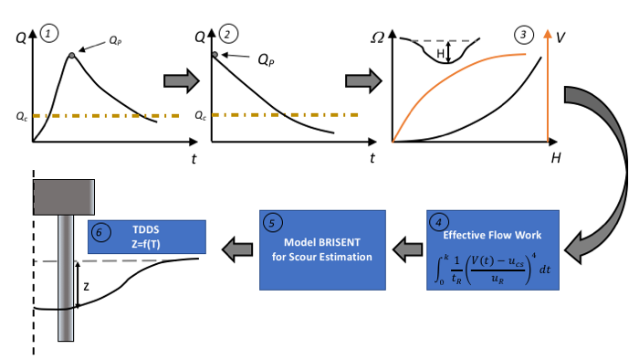
Given the experience from previous studies, it is known that the total scour is a function of the total flow work in a given location. Therefore, the proposed theoretical formulation can be extended to a case where the hydrograph assumes a complex or more realistic shape. With this aim, it is possible to redefine the mathematical formalism by assuming that the flood hydrograph is approximated by an exponential function. Figure 2 provides a conceptual diagram that includes the different steps adopted for the derivation of the TDDS.
In particular, one limitation that constrains the proposed approach is the fact that no hydrograph, in nature, is rectangular (a natural hydrograph is characterized by a raising limb and a recession phase). Therefore, the equivalent hydrograph of duration producing the same total work as the synthetic scour hydrograph is obtained by imposing:
Assuming that the flow hydrograph is represented by the NERC (Natural Environment Research Council) approximation [22],
the mean flow velocity is derived as,
Using the above formulation, the total work is defined as long as . Therefore, the upper limit of the integral is
The total associated to a random flood event with a synthetic exponential hydrograph becomes
and by imposing Equation (7), equals to Equation (21), and the parameter can be estimated as
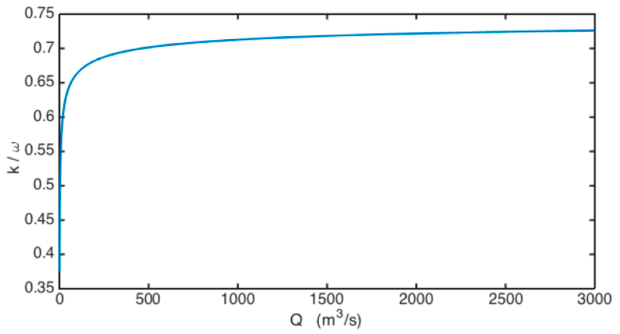
The duration of a rectangular hydrograph producing an equivalent scour as a real-shape hydrograph is clearly a function of . Equation (22) is depicted in Figure 3, where it is possible to clearly see how the parameter k/ rapidly reaches an asymptotic value, increasing the . The upper limit of the parameter is
Therefore, a possible approximation for the probability distribution of scour is represented by Equation (12), where the parameter can be derived using Equation (22). In this way, the total associated to each flood event is representative of an equivalent synthetic exponential hydrograph. It is worth underlining that the proposed expression for tends to overestimate the total duration of the equivalent rectangular hydrograph and it will produce a slightly conservative scour estimate.
4. Examples Applications
The proposed formulation offers an avenue to explore the interaction between floods and the scour process. It is especially interesting to explore the impact of some of the introduced parameters on the scour dynamics and also to illustrate a possible strategy to apply the formulation to a real case. It must be stated that we could not validate the results using real data because such field data were not available
4.1. Parameters of the BRISENT
BRISENT formulation relies on the principle of maximum entropy and on the stream power concept applied to local scour. It allows estimation of the scour depth evolution, under complex hydraulic scenarios, and has been tested on a significant number of laboratory data. Using this dataset, Pizarro et al. [13] derived a number of regression functions linking model parameters (, , and ) to physical characteristics of the study case. In particular, they observed that all these parameters can be related to one key parameter which is the ratio between the pier diameter and the characteristic sediment grain-size . Regression functions are:
4.2. Sensitivity Analysis
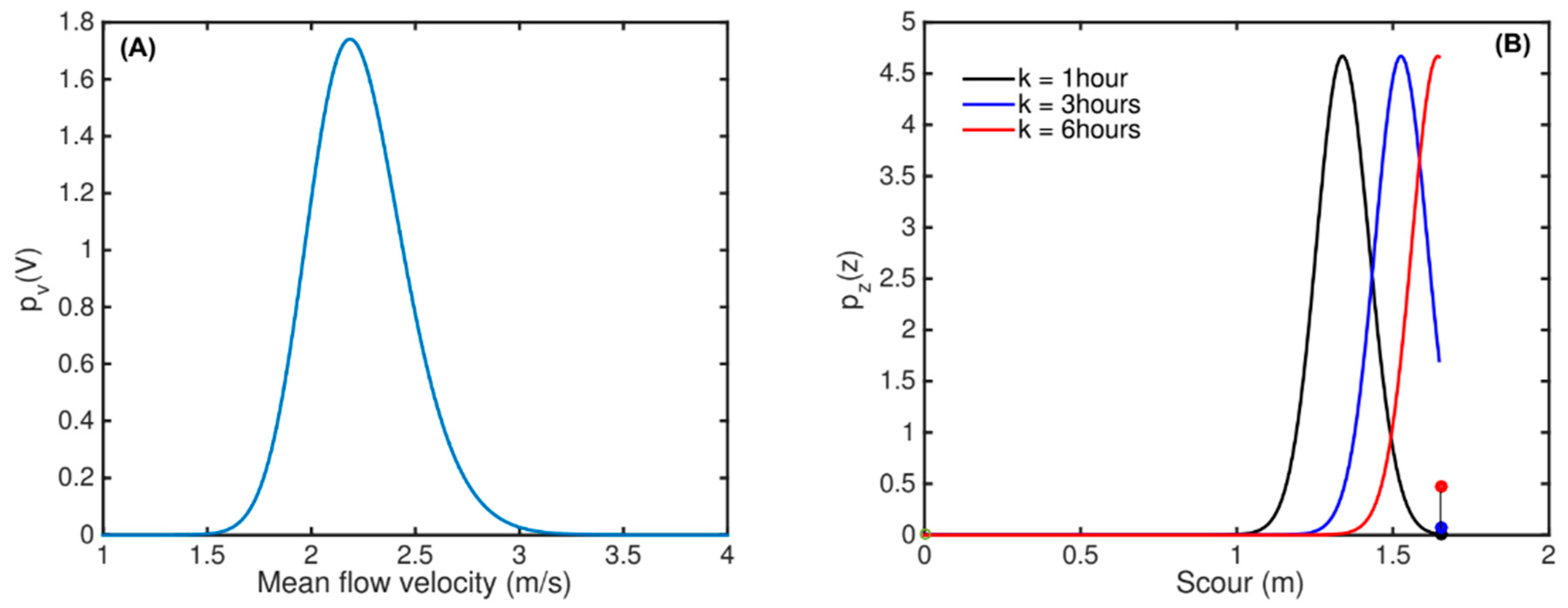
An example of the application of the proposed model is given in Figure 4, where the derived probability distributions of the mean flow velocities, associated with a specific configuration (panel A), and the associated probability distribution of scour depth obtained assuming different equivalent durations are depicted (panel B).
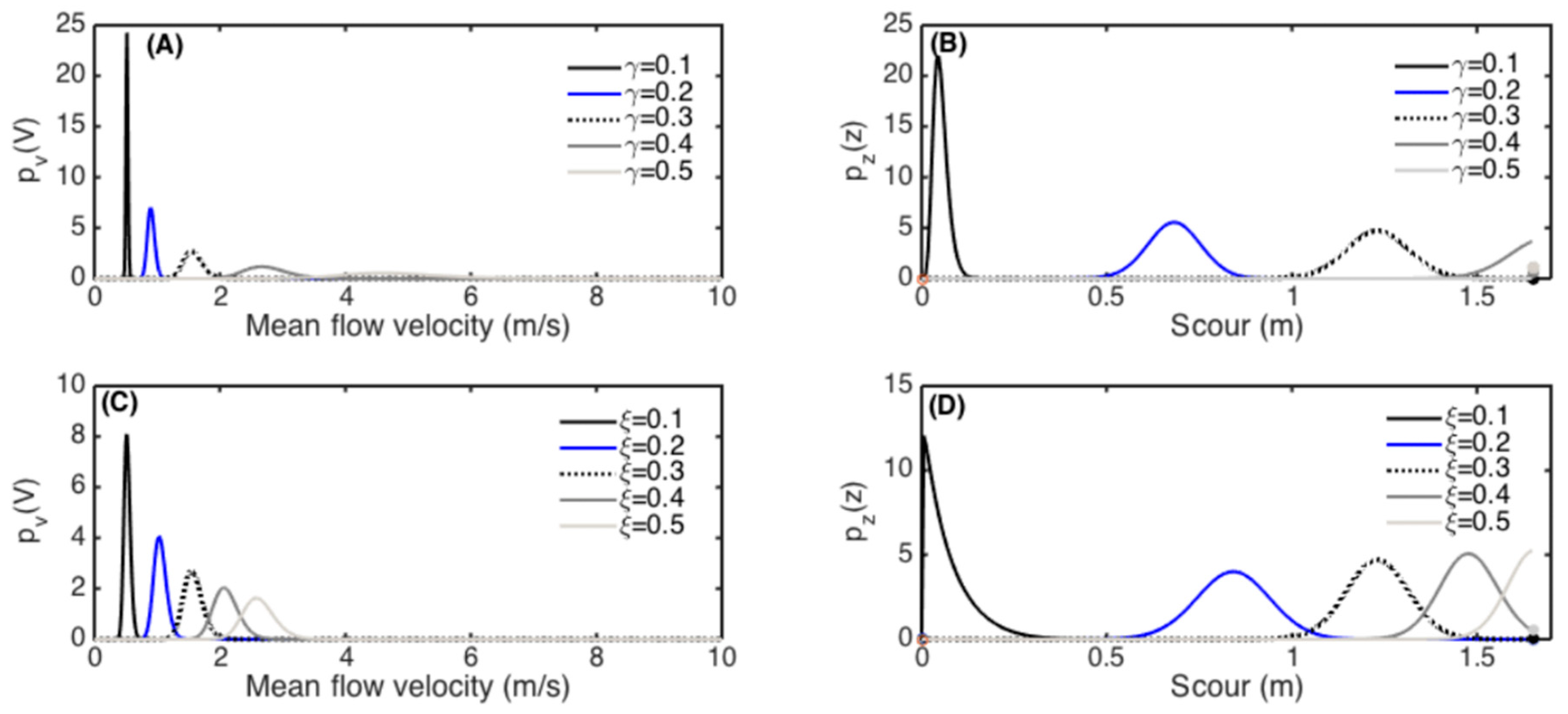
This graph makes it possible to underline the relative impact of hydrograph duration on the expected scour of a given cross-section. Complementary information, with respect to those previously described, are provided in Figure 5, where a description of the relative influence of the hydraulic parameters and , on the probability distribution of scour, is given using a similar set of parameters adopted from the previous figure.
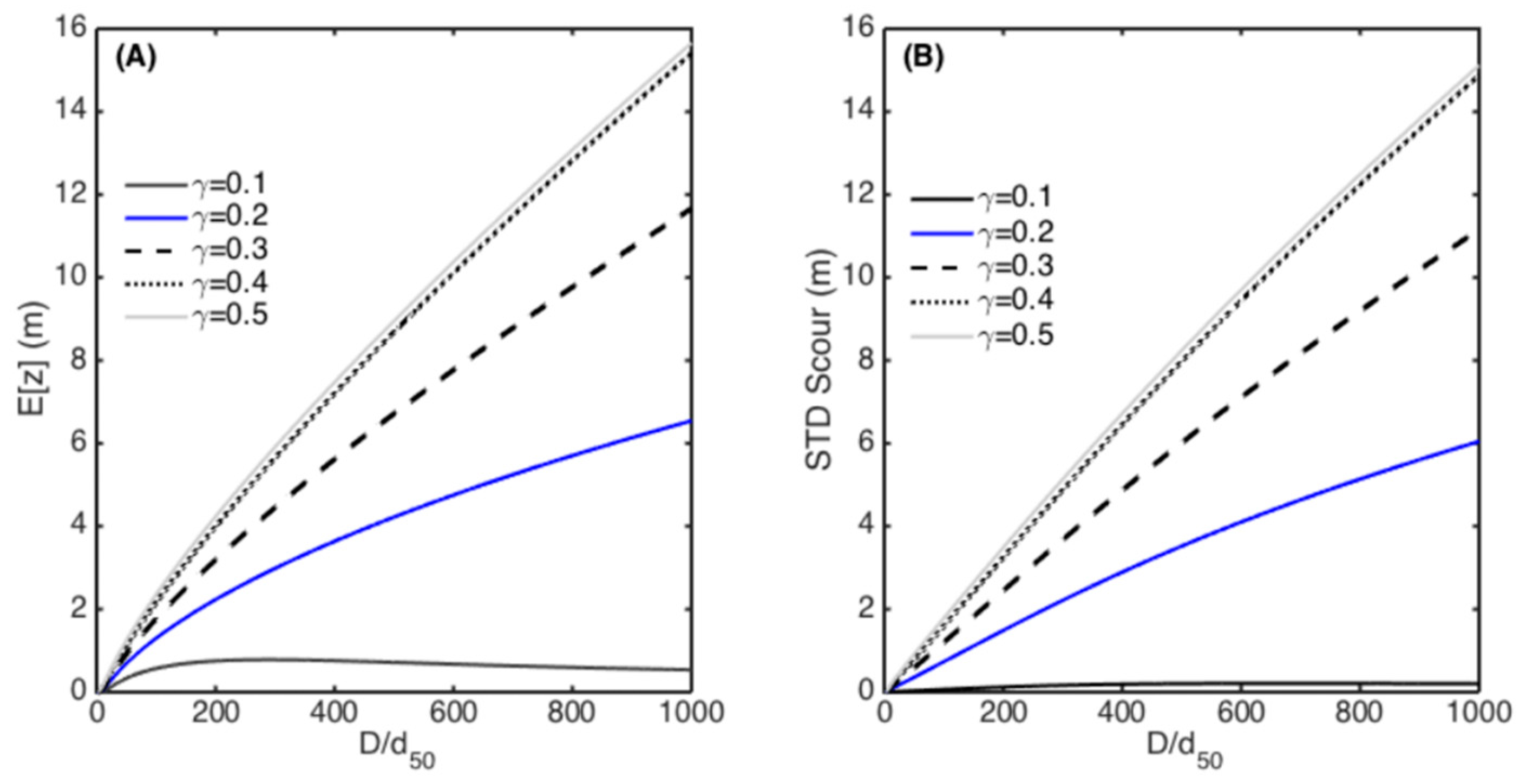
The proposed formulation is adopted to explore the role played by some critical parameters, such as the ratio between the pier diameter (D) and the sediment grain-size (ds) on the main statistics of scour. With this aim, Figure 6 provides a description of the mean and standard deviation of the scour depth as a function of the mentioned parameter, using different cross-section geometries. It can be noticed that both the mean and the variability of scour tend to increase monotonically with D/ds, except for the case with = 0.1. Moreover, the graph also clearly highlights the strong role played by the cross-section geometry on the overall dynamics of the process.
4.3. Application to a Real Context
The proposed formulation can be applied to different contexts, i.e., bridges already built to assess their vulnerability to scour, as well as in a design process. Up to now, bridge scour vulnerability assessment does not deal with a large number of scour data and consequently it is beneficial to use all the available information in this process. Therefore, we tried to exploit all available physical information in a real study case, to provide a realistic parametrization and application of the model.
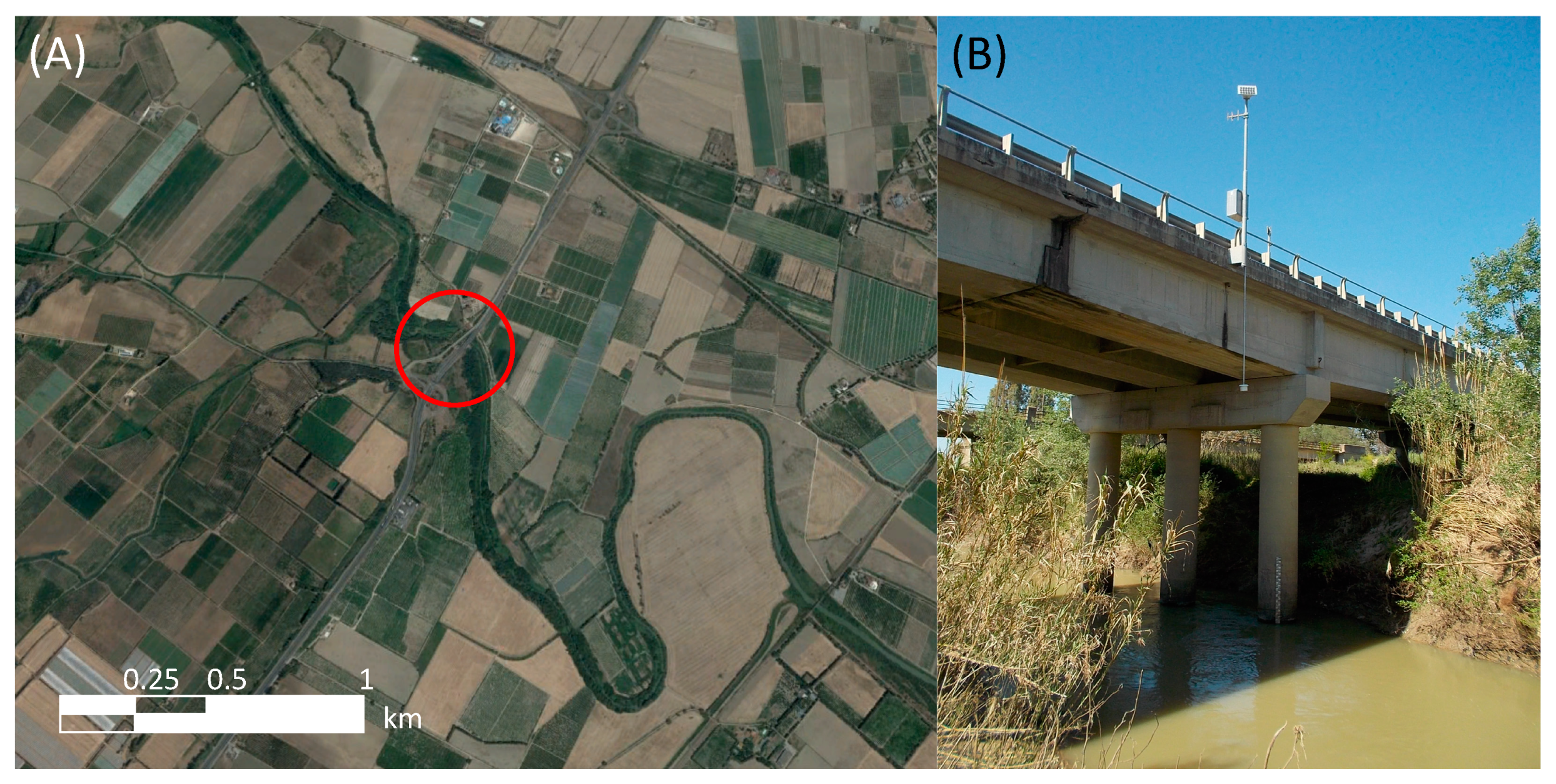
The TDDS formulation was tested by considering a bridge located on the Basento river in the Basilicata region (Southern Italy). Along with the bridge, there was a hydrometeorological station that provided all the needed information to carry out the analysis. The station, S.S. 106, drains an area of about 1520 km2 and has a mean annual discharge of about 141 m3/s. Figure 7 shows the case study with the location of the watershed and the river.
The main properties of the bridge and the study site, such as bridge length, number of piers, pier width, etc. are summarized in Table 1. The riverbed is composed of a uniform sediment having a d50 = 1.1 mm, which was used as a reference value for the ds.
TDDS was calibrated through the following steps:
- The parameters of the flood distribution were computed from the time series of annual maxima (Figure 8B). Several methods exist to estimate parameters of a Gumbel distribution; we used the method of moments for the sake of simplicity. Given the mean value was m3/s and the standard deviation was m3/s, Gumbel parameters were m3/s and m3/s
- Parameter k was estimated from recorded hydrographs. In the present case the duration of the hydrograph was set equal to 10 h.
- BRISENT parameters were estimated following Pizarro et al. [13]. Considering that the pier diameter was m and the grain-size was mm, the ratio reached a value of 1363.6. Using Equations (24)–(26), the BRISENT parameters were: , , and .
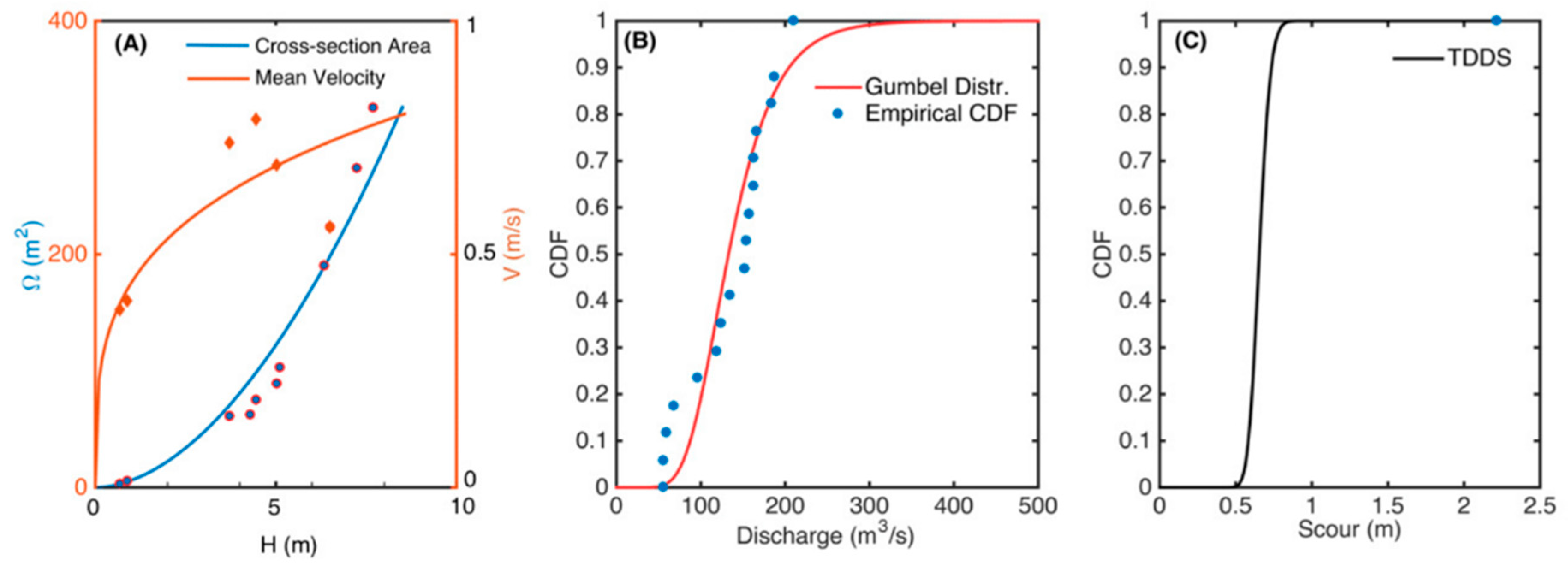
Figure 8 summarizes the different steps adopted during the model calibration to set hydraulic parameters (panel A), the probability distribution of floods (panel B), and finally the probability distribution of the scour (panel C).
The evaluation of risk for a bridge failure due to scour, through the proposed TDDS, is therefore crucial in reducing the uncertainty in bridge design. As shown through the study case on the Basento river, commonly available stream gauge records, as well as basic geometric properties of a bridge and the site curve of the riverbed sediments would allow for an application of the proposed TDDS.
Interestingly, the scour probability distribution is not just a simple transform of the flood probability function, but it is influenced by several factors, such as hydrograph shape, cross-section geometry, sediment, and bridge characteristics. Therefore, the actual bridge design conditions assumed nowadays, i.e., a 100-year discharge, might lead to unrealistic results, neglecting most of the complexity involved in the scour process.
5. Conclusions
Recent contributions regarding the treatment on bridge scour processes in unsteady hydraulic conditions are a cornerstone to reducing uncertainty in the hydraulic design of bridges and bridge scour assessment. These results have been exploited to provide a new theoretically derived probability distribution of scour (TDDS) that makes it possible to link, within a mathematical framework, the main variables involved in the process, such as river basin hydrology, hydraulic characteristics of the river, and characteristics of the cross-section, sediment, and pier. The proposed framework allows a better understanding of the impact of each of those components on scour depth probability distribution.
The model represents a new formalism to support bridge design, where all model parameters can potentially be linked to physical features. It is a simple and suitable approach to estimate flood-induced scour probability or conversely to estimate the risk of collapse (i.e., failure-risk associated with the probability of exceeding a given scour depth) of a given bridge, under specific conditions.
It would have been extremely interesting to test the proposed framework on a real study case, but the total absence of monitored data (in particular scour depth), over an extended temporal window, prevented such an attempt, however, it may potentially be tested on long-term numerical simulations and this task is currently under investigation. In the present study, we provided an example of application without the possibility to use real scour data with the aim to guide the readers in model parameter estimation.
In conclusion, it is worth noting that the proposed framework can be easily expanded using a different probability distribution of floods or eventually introducing the relative dependence between flood-peak discharge and the relative duration of the flood hydrograph.
Author Contributions
S.M. conceived and designed the research; O.L. and A.P. contributed to the conception and design of the study. All authors contributed to the overall framing and revision of the manuscript at multiple stages.
Funding
The authors recognize support of the European Commission, under the ELARCH program (Project Reference number: 552129-EM-1-2014-1-IT-ERA MUNDUS-EMA21), and the Chilean Consejo Nacional de Investigación Científica y Tecnológica CONICYT through the grants Fondecyt 1150997 and REDES 170021. This publication reflects the authors’ view only and the Commission is not liable for any use that may be made of the information contained herein.
Acknowledgments
We would like to thank reviewers for their insightful comments on the paper, as these comments led us to an improvement of the work.
Conflicts of Interest
The authors declare no conflict of interest.
Abbreviations
| a [m] | Coefficient of the power law cross-section area function of H |
| b[-] | Exponent of the power law cross-section area function of H |
| c [1/s] | Coefficient of the power law mean flow velocity function of H |
| d[-] | Exponent of the power law mean flow velocity function of H |
| [1/m2] | Coefficient of the power law mean flow velocity function of Q |
| [-] | Exponent of the power law mean flow velocity function of Q |
| [-] | location parameter of the Gumbel distribution |
| b1 [m3/s] | scale parameter of the Gumbel distribution |
| D [m] | Pier diameter |
| [m] | Sediment grain-size |
| g [m/s] | Acceleration of gravity |
| H [m] | Flow depth |
| k [s] | Duration of a rectangular hydrograph |
| [-] | BRISENT coefficient |
| [sec] | Characteristic time |
| [m2] | Cross-section area |
| pq(Q) [-] | Probability density function of floods |
| pv(V) [-] | Probability density function of velocities |
| pz*(Z*) [-] | Probability density function of dimensionless scour |
| pz(z) [-] | Probability density function of scour |
| Q [m3/s] | River discharge |
| Qmax [m3/s] | Maximum river discharge in a flood event |
| [kg/m3] | Relative density |
| [kg/m3] | Sediment density |
| [kg/m3] | Water density |
| S [-] | Entropic-scour parameter |
| t [s] | Time |
| tend [s] | Time in which a hydrograph is able to make work |
| tR [s] | Reference time |
| uc [m/s] | Critical velocity for the initiation of sediment motion |
| ucs [m/s] | Critical velocity for the incipient scour |
| uR [m/s] | Reference velocity |
| V [m/s] | Cross-section-averaged velocity |
| W* [-] | Dimensionless, effective flow work |
| W*max [-] | Maximum possible W*, according to BRISENT formulation |
| Z* [-] | Normalized scour depth |
| Z*max [-] | Maximum possible Z*, according to BRISENT formulation |
| zR [m] | Reference scour depth |
References
- Proske, D. Bridge Collapse Frequencies versus Failure Probabilities; Springer: Berlin/Heidelberg, Germany, 2018; ISBN 3319738321. [Google Scholar]
- Melville, B.W.; Coleman, S.E. Bridge Scour; Water Resources Publication: Littleton, CO, USA, 2000; ISBN 1887201181. [Google Scholar]
- Arneson, L.A.; Zevenbergen, L.W.; Lagasse, P.F.; Clopper, P.E. Evaluating Scour at Bridges (Hydraulic Engineering Circular No. 18, 5th ed.; FHWA-HIF-12-003; US DOT: Washington, DC, USA, 2012.
- Flint, M.M.; Fringer, O.; Billington, S.L.; Freyberg, D.; Diffenbaugh, N.S. Historical Analysis of Hydraulic Bridge Collapses in the Continental United States. J. Infrastruct. Syst. 2017, 23, 4017005. [Google Scholar] [CrossRef]
- Link, O.; Henríquez, S.; Ettmer, B. Physical scale modelling of scour around bridge piers. J. Hydraul. Res. 2018, 1–11. [Google Scholar] [CrossRef]
- Richardson, E.V.; Davis, S.R. Evaluating Scour at Bridges; Hydraulic Engineering Circular (HEC) No. 18; US DOT: Washington, DC, USA, 2001.
- Ettema, R.; Melville, B.W.; Constantinescu, G. Evaluation of Bridge Scour Research: Pier Scour Processes and Predictions; Transportation Research Board of the National Academies: Washington, DC, USA, 2011. [Google Scholar]
- Lu, J.-Y.; Hong, J.-H.; Su, C.-C.; Wang, C.-Y.; Lai, J.-S. Field measurements and simulation of bridge scour depth variations during floods. J. Hydraul. Eng. 2008, 134, 810–821. [Google Scholar] [CrossRef]
- Su, C.-C.; Lu, J.-Y. Comparison of Sediment Load and Riverbed Scour during Floods for Gravel-Bed and Sand-Bed Reaches of Intermittent Rivers: Case Study. J. Hydraul. Eng. 2016, 142, 5016001. [Google Scholar] [CrossRef]
- Hager, W.H.; Unger, J. Bridge pier scour under flood waves. J. Hydraul. Eng. 2010, 136, 842–847. [Google Scholar] [CrossRef]
- Guo, J. Semi-analytical model for temporal clear-water scour at prototype piers. J. Hydraul. Res. 2014, 52, 366–374. [Google Scholar] [CrossRef]
- Link, O.; Castillo, C.; Pizarro, A.; Rojas, A.; Ettmer, B.; Escauriaza, C.; Manfreda, S. A model of bridge pier scour during flood waves. J. Hydraul. Res. 2017, 55. [Google Scholar] [CrossRef]
- Pizarro, A.; Samela, C.; Fiorentino, M.; Link, O.; Manfreda, S. BRISENT: An Entropy-Based Model for Bridge-Pier Scour Estimation under Complex Hydraulic Scenarios. Water 2017, 9, 889. [Google Scholar] [CrossRef]
- Pizarro, A.; Ettmer, B.; Manfreda, S.; Rojas, A.; Link, O. Dimensionless effective flow work for estimation of pier scour caused by flood waves. J. Hydraul. Eng. 2017, 143. [Google Scholar] [CrossRef]
- Manfreda, S. On the derivation of flow rating-curves in data-scarce environments. J. Hydrol. 2018, 562, 151–154. [Google Scholar] [CrossRef]
- Hamed, K.; Rao, A.R. Flood Frequency Analysis; CRC Press: Boca Raton, FL, USA, 1999. [Google Scholar]
- Iacobellis, V.; Fiorentino, M.; Gioia, A.; Manfreda, S. Best Fit and Selection of Theoretical Flood Frequency Distributions Based on Different Runoff Generation Mechanisms. Water 2010, 2, 239–256. [Google Scholar] [CrossRef] [Green Version]
- Cunnane, C. Methods and merits of regional flood frequency analysis. J. Hydrol. 1988, 100, 269–290. [Google Scholar] [CrossRef]
- Fiorentino, M.; Gabriele, S.; Rossi, F.; Versace, P. Hierarchical Approach for Regional Flood Frequency Analysis. Reg. Flood Freq. Anal. 1987, 3549. Available online: http://www.diia.unina.it/pdf/pubb0550.pdf (accessed on 23 October 2018).
- Hosking, J.R.M.; Wallis, J.R. Some statistics useful in regional frequency analysis. Water Resour. Res. 1993, 29, 271–281. [Google Scholar] [CrossRef]
- Smith, A.; Sampson, C.; Bates, P. Regional flood frequency analysis at the global scale. Water Resour. Res. 2015, 51, 539–553. [Google Scholar] [CrossRef] [Green Version]
- Natural Environmental Research Council (NERC). Estimation of Flood Volumes over Different Duration. In Flood Studies Report; NERC: London, UK, 1975; Volume I, pp. 352–373. [Google Scholar]
Figure 1.
Example of different cross-sections described with different values of (A), the corresponding flow rating curve (B) and the velocity as a function of the discharge (C). Parameter a and parameter b are defined on the basis of the assigned value of , while the remaining parameters are a = 2, b = 1 and c = 0.2.

Figure 2.
Conceptual diagram illustrating the different steps of TDDS derivation: (1) The natural flood hydrograph; (2) the equivalent exponential hydrograph; (3) the use of the mean flow velocity function to derive the scour energy; (4) estimation of the effective flow work; (5) derivation of the total scour at the event scale; and (6) derivation of the probability distribution of scour.
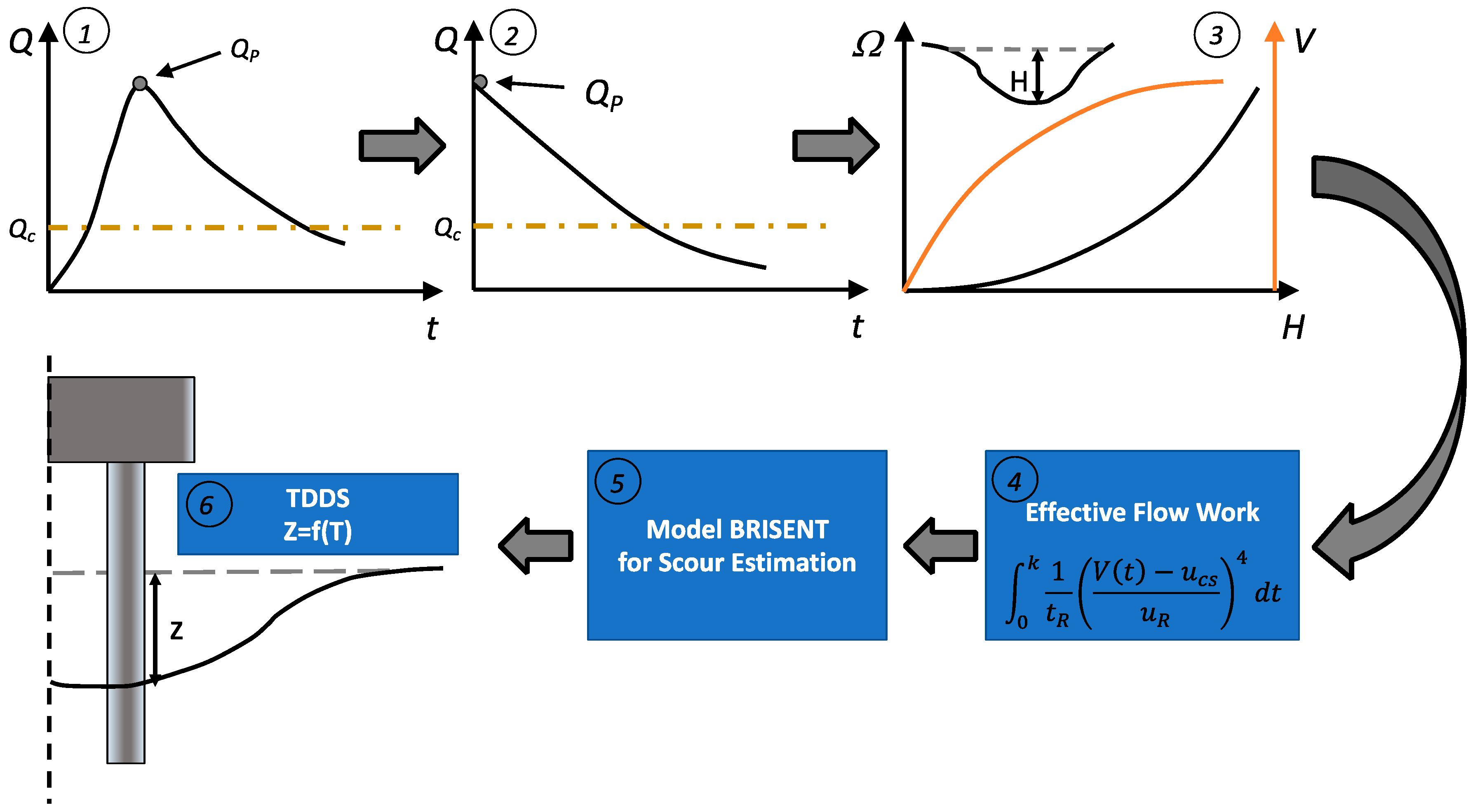
Figure 3.
Ratio between equivalent duration k and as a function of the discharge. It can be noticed that the ratio k/ tends to stabilize when Q tends to increase.
Figure 3.
Ratio between equivalent duration k and as a function of the discharge. It can be noticed that the ratio k/ tends to stabilize when Q tends to increase.

Figure 4.
Derived probability density function of the mean flow velocities associated with a given river basin (A) and the corresponding PDFs of scour depth (B) obtained assuming hydrographs with variable equivalent duration k, ranging from 1 to 6 h. Other parameters are: D = 1.07 m; d50 = 0.001 m; = 2.65 t/m3; uc = 0.319 m/s; = 4.7252 × 10³; W*max = 1.8613 × 10⁵; S = 8.9026; α = 67.8627 m3/s; b1 = 143.643; = 0.33; = 0.36 1/m2.

Figure 5.
Derived probability density functions of the mean flow velocities associated with a given river basin (A,C) and the corresponding PDFs of scour depths obtained by modifying the shape parameter of the cross-section γ, with a fixed value of = 0.30 1/m2 and k = 60 min (A,B), or modifying the scale parameter with fixed values of γ = 0.30 and k = 60 min (C,D). Other parameters are: D = 1.07 m; d50 = 0.001 m; = 2.65 t/m3; uc = 0.319 m/s; = 4.7252 × 10³; W*max = 1.8613 × 10⁵; S = 8.90; α = 67.86 m3/s; b1 = 143.64.

Figure 6.
Mean (A) and standard deviation (B) of scour obtained with the proposed framework for different cross-sections, obtained by modifying the shape parameter of the cross-section γ. Other parameters are: D = 1.07 m; d50 = 0.001 m; = 2.65 t/m3; uc = 0.319 m/s; = 4.7252 × 10³; W*max = 1.8613 × 10⁵; S = 8.90; α = 67.86 m3/s; b1 = 143.64; = 0.30 1/m2 and k = 60 min.

Figure 7.
Description of the case study adopted: (A) Aerial photo and (B) photo of the bridge (lat: 40.36°; lon: 16.78°).
Figure 7.
Description of the case study adopted: (A) Aerial photo and (B) photo of the bridge (lat: 40.36°; lon: 16.78°).

Figure 8.
TDDS derived for a real study case: (A) Hydraulic function of velocity and cross-section area as a function of the hydraulic stage H; (B) cumulated probability distribution of flood annual maxima; (C) cumulated probability distribution of scour of the Basento River at SS106.
Figure 8.
TDDS derived for a real study case: (A) Hydraulic function of velocity and cross-section area as a function of the hydraulic stage H; (B) cumulated probability distribution of flood annual maxima; (C) cumulated probability distribution of scour of the Basento River at SS106.


Table 1.
Main characteristics of the selected study case.
| Description | Data |
|---|---|
| Cross-section | Basento SS 106 |
| River Basin Area (km2) | 1520 |
| E[Q] (m3/s) | 141 |
| σ[Q] (m3/s) | 49 |
| Pier Diameter D (m) | 1.5 |
| Sediment Size d50 (mm) | 1.1 |
| Number of Piers | 4 |
| Bridge Length (m) | 15 |
© 2018 by the authors. Licensee MDPI, Basel, Switzerland. This article is an open access article distributed under the terms and conditions of the Creative Commons Attribution (CC BY) license (http://creativecommons.org/licenses/by/4.0/).
Share and Cite
MDPI and ACS Style
Manfreda, S.; Link, O.; Pizarro, A. A Theoretically Derived Probability Distribution of Scour. Water 2018, 10, 1520. https://doi.org/10.3390/w10111520
AMA Style
Manfreda S, Link O, Pizarro A. A Theoretically Derived Probability Distribution of Scour. Water. 2018; 10(11):1520. https://doi.org/10.3390/w10111520
Chicago/Turabian StyleManfreda, Salvatore, Oscar Link, and Alonso Pizarro. 2018. "A Theoretically Derived Probability Distribution of Scour" Water 10, no. 11: 1520. https://doi.org/10.3390/w10111520
Note that from the first issue of 2016, this journal uses article numbers instead of page numbers. See further details here.