Mathematical Modeling of Non-Fickian Diffusional Mass Exchange of Radioactive Contaminants in Geological Disposal Formations

1
Institute of Fluid Science, Tohoku University, Sendai, Miyagi 980-8577, Japan
2
Department of Mathematics and Statistics, California State University, Chico, CA 95929, USA
3
Institute of Mathematics, Informatics and Natural Sciences, Moscow City University, 129226 Moscow, Russia
4
Fracture & Reliability Research Institute, School of Engineering, Tohoku University, Sendai, Miyagi 980-8579, Japan
*
Author to whom correspondence should be addressed.
†
Current address: 2-1-1 Katahira, Aoba-ku, Sendai, Miyagi 980-8577, Japan.
Water 2018, 10(2), 123; https://doi.org/10.3390/w10020123
Submission received: 30 July 2017
/
Revised: 8 January 2018
/
Accepted: 23 January 2018
/
Published: 29 January 2018
(This article belongs to the Special Issue Advances in Groundwater Flow and Solute Transport: Pushing the Hidden Boundary)
Abstract
:Deep geological repositories for nuclear wastes consist of both engineered and natural geologic barriers to isolate the radioactive material from the human environment. Inappropriate repositories of nuclear waste would cause severe contamination to nearby aquifers. In this complex environment, mass transport of radioactive contaminants displays anomalous behaviors and often produces power-law tails in breakthrough curves due to spatial heterogeneities in fractured rocks, velocity dispersion, adsorption, and decay of contaminants, which requires more sophisticated models beyond the typical advection-dispersion equation. In this paper, accounting for the mass exchange between a fracture and a porous matrix of complex geometry, the universal equation of mass transport within a fracture is derived. This equation represents the generalization of the previously used models and accounts for anomalous mass exchange between a fracture and porous blocks through the introduction of the integral term of convolution type and fractional derivatives. This equation can be applied for the variety of processes taking place in the complex fractured porous medium, including the transport of radioactive elements. The Laplace transform method was used to obtain the solution of the fractional diffusion equation with a time-dependent source of radioactive contaminant.
1. Introduction
High-level nuclear wastes are a by-product of nuclear power generation and other applications of nuclear fission or nuclear technology which must be shielded from humans and the environment for a long time. Subsurface nuclear waste repositories consist of engineered and geological barriers that isolate the radioactive materials from the human environment. If the radioactive contaminants leak to aquifers, the damage would be serious because it directly contaminates our drinking water. We need to answer how and when the contaminants leak from the power plants or the waste repositories unintentionally, and how much they affect human beings and the natural environment. Safe disposal of nuclear wastes requires an evaluation of the risks of contaminants for aquifers and prediction of the possible migration of contaminated groundwater.
Fluid flow and contaminant transport in aquifers are dominated by fractures and large pores. Numerous studies indicate that the real nature of solute transport in geological formations exhibits anomalous behavior [1,2,3,4]. Multiscale subsurface systems often produce power-law tails in breakthrough curves [5,6,7,8], as well as in a nuclear waste repository site [9]. The breakthrough curves are not adequately described by the typical advection-dispersion with an exponential residence time (e.g., [10,11]).
Problems of solute transport in a single fracture-matrix system have been addressed, and the analytical solutions have been developed based on the advection-dispersion equation [12,13]. Alternative transport models are proposed to capture the effects of spatial heterogeneities in fractured rocks and the effects of flow channeling or velocity dispersion [14,15]. The models have extended to the mass transfer models with time- or space-dependent dispersion coefficients (e.g., [16]), the multi-rate mass transfer models [17], the continuous time random walk approach [18], the time-domain random walk approach, the fractional advection-dispersion equation approach [19], and the stochastic approach [20].
The fractional derivative can be understood as a convolution of an integer-order derivative with a memory function [21], and the time convolution can capture memory effects, allowing particles to reside for long periods. The temporal fractional derivatives can produce power law residence times of solute transport. Liu et al. [22] considered the time fractional advection-dispersion equation, and the solution was obtained by using variable transformation. Fomin et al. [23] studied mass transport in a fractured-porous aquifer (i.e., aquifer filled with porous blocks) and modeled the effects of interaction with porous blocks in the aquifer by temporal fractional derivatives. Numerical study shows that varying the variations of order of fractional derivatives enables the description of different power law decays obtained from a homogeneous porous medium to a fractured medium [24].
This study proposes a mathematical model of radioactive contaminant transport in a single fracture within a confining porous matrix. Usually, sources of radioactive contamination vary with time. For example, an exponentially decaying source boundary condition is frequently used in radioactive waste disposal or non-aqueous phase liquid sites [25]. We derive the universal equation of mass transport for dissolved molecular size contaminants within a fracture, which accounts for the complexity of the confining porous matrix and temporal decay of the contaminant concentration. In this equation, the specific features of mass transport in the surrounding matrix and mass exchange between the fracture and matrix are modeled by the special function , which represents the integral of convolution. This paper provides the analytic derivation of the function in its most general form, so that the majority of the well documented models can be obtained as particular cases of the presented model. For example, in the absence of radioactive decay, the solution presented in this paper reduces to the solution obtained by Fomin et al. [23] for and . When mass flux is Fickian with and , the solution was obtained by Tang et al. [12], which also follows as a particular case from the solution obtained in this paper.
2. Model
2.1. Governing Equation
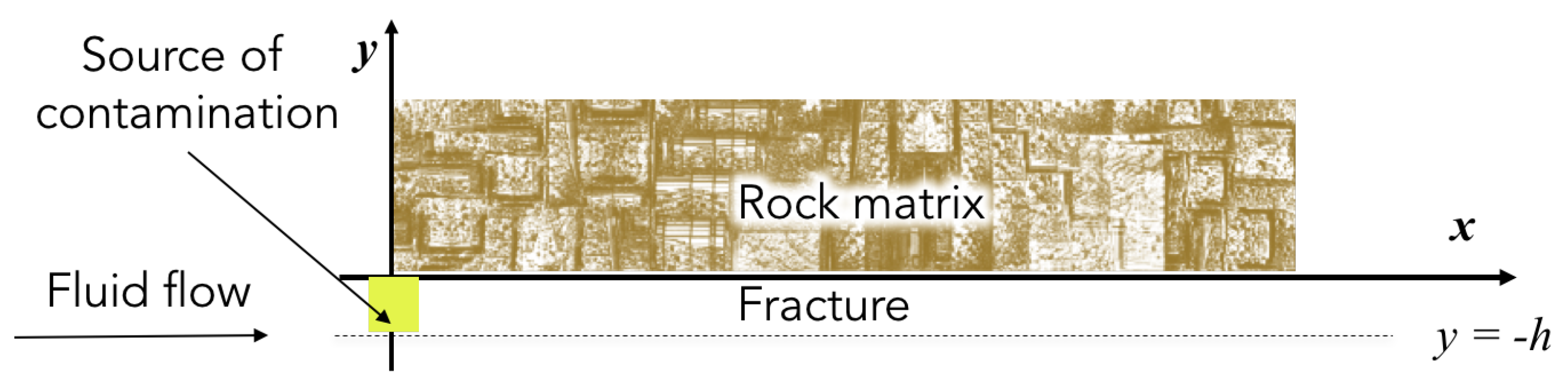
We consider radioactive solute transport in a single fracture surrounded by porous rocks. The fracture does not contain any porous inclusions, which is different from the concept in the previous study [23]. A schematic sketch of a fracture and rock matrix is presented in Figure 1. A parallel plate fracture is confined by porous rocks, which have same physical properties for the upper and lower sides. Cartesian coordinates (x, y) are chosen in such a manner that fluid in the fracture flows in the x-direction and that the coordinate y is perpendicular to the x-direction. Transport processes can be symmetrical with regard to the median line of the fracture at (dashed line in Figure 1). This leads to the mass flux of 0 at , and the solutions in the sub-domains below and above this line are identical. Thus, we can only consider the upper half of the domain ().
Let and be the concentrations of the solute within the porous matrix and the fracture, respectively. We consider only dissolved molecular-size contaminants, not suspended particles in the aqueous phase radioactive particles. Because the thickness of the fracture is much smaller than its length, the mean concentration of the solute within the fracture can be given by . Mass transport in this system consists of (i) advection and (ii) diffusion in the fracture, (iii) absorption on the fracture walls, (iv) diffusion into the surrounding rocks, (v) adsorption on the walls of the pores in the surrounding rocks, and (vi) radioactive decay of radioactive contaminants both in fracture and porous matrix. Each governing equation within the fracture and within the rock matrix can be written as [12]:
where is time. s and are the mass of the solute adsorbed on the walls of the fracture and pores in the rock matrix, respectively. v is the average velocity of the solution in the fracture. D and are the effective diffusivities in the fracture and in the porous medium, respectively, which include dispersion and molecular diffusion in the fracture and in the porous medium. is a radioactive decay constant. q is the mass flux on the wall of the fracture. is the density of the rock matrix, and is the matrix porosity.
It has been observed that pore spaces and micro-cracks in the rock matrix are distributed in various sizes and different orientations [26]. We assume that contaminants not only penetrate in the matrix due to molecular diffusion, but also migrate through micro-cracks due to advection. Thus, the effective diffusivity, , accounts for dispersion and molecular diffusion. If micro-cracks within the surrounding matrix have an orientation perpendicular to the conducting fracture, contaminants may migrate long distances and lead to a faster process than diffusion (super diffusion). We should predict the worst scenario to evaluate the risks of contaminants’ migration. Thus, in order to account for the advective process in the surrounding rocks, this study used the generalized Fickian mass flux in the matrix by introducing a fractional derivative, in the following form [27]:
where is the order of fractional derivative (). The value of leads to faster (superdispersive) spreading, while the value of causes slower (subdiffusive) spread [25]. Equation (3) describes Fickian diffusion when the index on space fractional derivative is 1/2 (i.e., ). The fractional derivative can be defined by means of Laplace transformation , from the equation , which is equivalent to the Caputo definition [28], .
The relationship between c and s in Equation (1) and between and in Equation (2) can be assumed [12] as
where and are given constants. Substituting correlations (4) and (5) into Equations (1) and (2) yields
where and are retardation coefficients.
In general, concentration in the matrix is a function of both spatial coordinates, x and y: . Let l and h be the characteristic scales for the length in the x-direction (along the aquifer) and y-direction, respectively. The scale l is defined by the distance of contaminant intrusion into the aquifer in the x-direction due to the advective transport, and the scale h is defined by the thickness of the aquifer. The characteristic values of the concentration gradient in x- and y-direction are and , respectively. Therefore, the ratio of the gradients can be estimated by the quotient of the length scales, . Obviously, the scale l can be much greater than the scale h, and the ratio can be very small. Hence, diffusion in the x-direction is negligibly small compared to the diffusion in y-direction. Thus, the derivative of with respect to x is ignored. This is the same assumption with Grisak and Pickens [29] and Tang et al. [12]. Dependence of on x is a consequence of the boundary conditions on the rock–fracture interface (), which couples with the mean concentration in the fracture, c.
In order to generalize the equations, the non-dimensional forms are derived with the proper characteristic scales. The scale for time represents the characteristic time for contaminant penetration in the rock matrix to the distance h, given by . The scale for the variable x-coordinate along the fracture is the characteristic distance of contaminant migration by the characteristic time , described as . The scale for the y-coordinate is defined to be half of the aquifer, h. The initial concentration of solute at the inlet where the source of contamination is located, (0), can be used as the scale for solute concentration. Based on these scales, non-dimensional variables can be introduced as follows:
Substituting the non-dimensional variables in Equation (8) into Equations (6) and (7) yields the following:
The following boundary and initial conditions can be imposed:
where is the non-dimensional concentration at the inlet of the fracture. Typically, the concentration distribution in the aquifer can be approximated by a parabola. Therefore, the maximum values of concentration can be reached in the middle of the aquifer, while the lowest values at the aquifer–matrix interface. In this case, assuming that the concentration on the interface is equal to the mean concentration C in the aquifer (the boundary condition (15)), which slightly overestimates the concentration on the border of the matrix. Therefore, the computed concentration in the region will be slightly overestimated. However, using the present model as a tool for predicting contamination in the real world situations, the slight overestimation of the possible hazardous contamination is a positive factor.
2.2. Analytical Solution
Equation (9) describes mass transport in a fracture, which contains the variables C and (i.e., concentration in the fracture and in the matrix, respectively). Let us consider the mass flux on the fracture–matrix interface on the right hand side in Equation (9), which can be written by:
Based on an analogy of Duhamel’s theorem [30], the solution for the concentration in the matrix, , can be coupled with the concentration in the fracture, C, by the following equation:
where the function in Equation (17) is a solution of the following auxiliary problem:
The mass flux in Equation (18) is given by:
Mass flux differentiations, Q given by Equation (16) and given by Equation (22), are performed with respect to the variable Y, whereas the differentiation and the integration in Equation (17) are performed with respect to the variables t and , respectively. We can change the order of fractional differentiation with respect to Y to the order of differentiation with respect to t and the order of integration with respect to . As a result, we obtain
where does not depend on Y. In addition, the mass flux Q given by Equation (23) can be rewritten in the form:
where
Substituting Equations (23) and (24) into Equation (9) leads to the following boundary value problem for C (i.e., concentration in the fracture):
Equation (26) describes the majority of the transfer processes in the fracture and the specific feature of mass exchange between the fracture and the matrix. The derivation can be done by constructing the appropriate function in Equation (25).
Applying the technique of the group analysis of differential equations [31], the solution of the formulated boundary-value problem (18)–(21) can be obtained in the following form [23]:
where . is Gamma function. This expression follows from (2.17)–(2.32) in [23] at .
From Equation (30), it follows that
where . Accounting for Equations (22) and (31), Equation (25) leads to the following expression:
where is an incomplete Gamma function. Equation (32) represents the mass flux on the wall of the fracture when on the fracture wall.
Let us consider particular cases. If and were 0, mass exchange does not occur at the fracture–matrix interface. Then, the problem is reduced to the problem in [12]. If no radioactive decay occurs (i.e., ) and diffusion is Fickian (i.e., ), . According to the definition of the fractional derivative [28], Equation (24) can be written as . If no radioactive decay occurs (i.e., ) but diffusion is described by the generalized Fick’s law (3) (i.e., ), the mass fluxes can be given as and . When is small and time is , formula (32) approaches the following asymptotic representation:
The accuracy of this asymptotic formula can be easily verified by simple numerical computations. Our computations show that the difference between the values of computed by Equations (32) and (33) is negligibly small within the relatively long time interval from 0 to and [23]. Thus, Equation (33) can be used as a good approximation for , the exact value of which is given by Equation (32). Using formula (33), the mass flux Q defined by Equation (24) can be presented through the fractional derivatives:
Let us turn to solution of the boundary value problem (26)–(29). In the case where , and converting to originals, we obtain
Or, in the case where , then
Equations (35) and (36) are well-known solutions in [12,14]. Solution (36) does not follow from (35), while solution (35) follows from (36) at .
The function at the right hand side in Equation (26) is given by Equation (33). If the time range is from 0 to for Equation (26), it is convenient to rescale Equation (26) with new time variable . In this case, the new spatial variable should be defined as . With these new non-dimensional variables, Equation (26) can be presented in the following form:
where , , , and . Note that the expression for can be presented as , according to Equation (33). The third term at the left hand side in Equation (37) including describes diffusion in the fracture. Because and , parameter in Equation (37) is small (). Hence, in major cases within time of the order of , the effects of the diffusive transport in the fracture is negligible. Equation (37) can be rewritten as follows:
3. Results
First, we consider the case where the concentration at the inlet is constant (i.e., and ). For this case, let us describe the concentration as . The inverse Laplace transformation leads to the following expression:
where is a Heaviside step function and
when concentration in the inlet is an arbitrary function of T (i.e., ), then concentration in the fracture can be obtained by utilizing Duhamel’s theorem [30]:
where is the concentration when the concentration at the inlet is constant, defined by Equation (42). If the radioactivity decays exponentially at the inlet, the boundary concentration and its Laplace form are given as and . The solution C can be obtained by the inverse Laplace transform directly from Equation (41) as:
where
The effects of the order of fractional derivatives on radioactive contaminant transportation are shown in Figure 2 and Figure 3. Analytical solutions for the constant concentration at the inlet given by Equation (42) are plotted for different in Figure 2a,b. The initial concentration is , and the boundary source concentration at is . As shown in Figure 2a, concentrations at far points from the inlet were larger for than that for . For the case of larger , contaminants are most likely to migrate through the fracture. In contrast, small describes transport with longer delays, which derive from diffusion into the surrounding rocks or adsorption and desorption to the fracture walls. Thus, smaller describes a longer memory effect.
The mass flux on the fracture–matrix interface in Equation (3) is taken account for the generalized Fick’s law with fractional spatial derivative, and does not describe the effect of temporal memory. However, since we deal with the mass flux on the fracture–matrix interface where the concentration of the transported contaminant significantly depends on time, it is physically obvious that the mass flux at the given moment of time depends not only on concentration at this moment of time, but also on how this concentration varied in the previous moment of time. This feature can be called the effect of temporal memory and mathematically described by the convolution integral in Equation (24). Equation (31) also explains that the generalized Fick’s law with fractional spatial derivative accounts for the memory effect. Incidentally, Equation (24) allows the mixed problems of calculating concentration on the fracture–matrix interface to be split into separate problems of calculating concentration in the matrix and calculating concentration in the fracture, respectively. The latter significantly simplifies the analysis of mass transport in the matrix–fracture system.
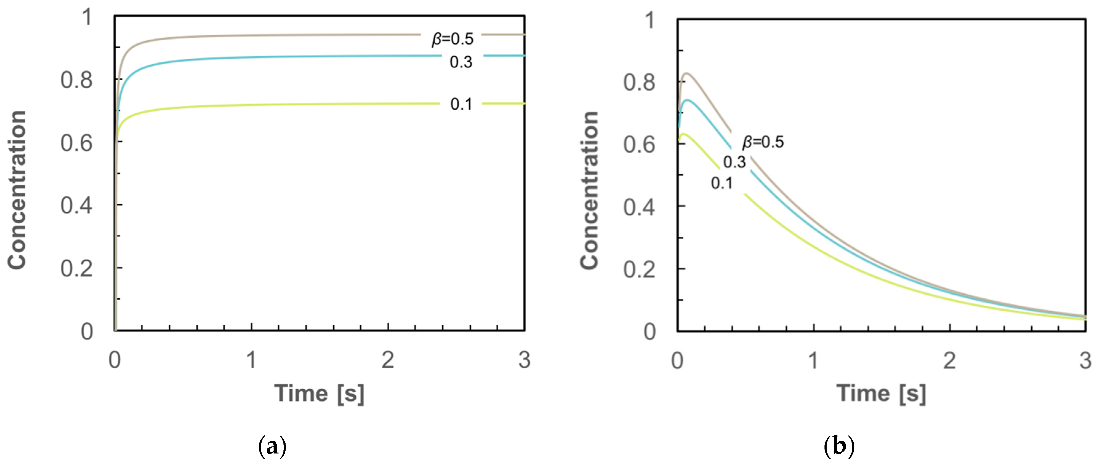
As shown in Figure 3a, concentration for constant boundary source approached certain values of concentration, which did not reach the injected concentration (). We can see that larger shows larger concentration at the late time, showing the phenomenon of longer memory as discussed above.
Analytical solutions for the time-dependent boundary sources given by Equation (45) are plotted for different in Figure 2b and Figure 3b. With the same conditions as above, the initial concentration is . The boundary source was set to time-dependent . Concentration at was 1 for constant boundary source (Figure 2a), while concentration for time-dependent boundary source started from 0.37 when (Figure 2b). In the case of the time-dependent boundary source, concentrations decayed at the late time.
4. Conclusions
We derived the analytical solution of the boundary value problem (26)–(29) for radioactive contaminant transport through a fracture. By deriving the formula (24), This formula allows the mixed problems of calculating concentration on the fracture–matrix interface to be split into separate problems of calculating concentration in the matrix and calculating concentration in the fracture, respectively. The latter significantly simplifies the analysis of mass transport in the matrix–fracture system. When the solute concentration at the inlet is constant, the concentration in the fracture can be obtained by Equation (42). When the source boundary concentration at the inlet decays exponentially, the concentration in the fracture can be obtained by Equation (45). We plotted the analytical solutions for different values of , which indicate that the value of allows the evaluation of the residence time of contaminants in the aquifer. This analysis, based on the analytical solutions of fractional diffusion equation, can provide simple and quick results to evaluate solute transport in fractured rocks. Most of the cases where radioactive contaminants cause troubles would be in unexpected situations. At that time, the simple and quick analysis proposed by this research will help instant management strategies.
Acknowledgments
This work was supported by the Japan Society for the Promotion of Science, under Grant-in-Aid for Young Scientists(A)(717H049760), whose support is gratefully acknowledged.
Author Contributions
Sergei Fomin, Vladimir Chugunov, and Anna Suzuki contributed to the development of the mathematical model and derivation of the analytical solutions. Anna Suzuki and Toshiyuki Hashida solved numerically the analytical solutions, and Anna Suzuki wrote the paper.
Conflicts of Interest
The authors declare no conflict of interest.
Appendix A
References
- Coats, K.; Smith, B.D. Dead-end pore volume and dispersion in porous media. Soc. Petrol. Eng. J. 1964, 4, 73–84. [Google Scholar] [CrossRef]
- Long, J.C.S.; Remer, J.S.; Wilson, C.R.; Witherspoon, P.A. Porous media equivalents for network of discontinuous fractures. Water Resour. Res. 1982, 18, 645–658. [Google Scholar] [CrossRef]
- Sahimi, M. Flow phenomena in rocks: From continuum models to fractals, percolation, cellular automata, and simulated annealing. Rev. Mod. Phys. 1993, 65, 1395–1534. [Google Scholar]
- Edery, Y.; Guadagnini, A.; Scher, H.; Berkowitz, B. Origins of anomalous transport in heterogeneous media: Structural and dynamic controls. Water Resour. Res. 2014, 50, 1490–1505. [Google Scholar] [CrossRef]
- Hatano, Y.; Hatano, N. Dispersive transport of ions in column experiments: An explanation of long-tailed profiles. Water Resour. Res. 1998, 34, 1027–1033. [Google Scholar] [CrossRef]
- Haggerty, R.; Wondzell, S.M.; Johnson, M.A. Power-law residence time distribution in the hyporheic zone of a 2nd-order mountain stream. Geophys. Res. Lett. 2002, 29, 1640. [Google Scholar] [CrossRef]
- Radilla, G.; Sausse, J.; Sanjuan, B.; Fourar, M. Interpreting tracer tests in the enhanced geothermal system (EGS) of Soultz-sous-Forêts using the equivalent stratified medium approach. Geothermics 2012, 44, 43–51. [Google Scholar] [CrossRef]
- Cardenas, M.B.; Slottke, D.T.; Ketcham, R.A.; Sharp, J.M., Jr. Navier-Stokes flow and transport simulations using real fractures shows heavy tailing due to eddies. Geophys. Res. Lett. 2007, 34, L14404. [Google Scholar] [CrossRef]
- Hodgkinson, D.; Benabderrahmane, H.; Elert, M.; Hautojärvi, A.; Selroos, J.O.; Tanaka, Y.; Uchida, M. An overview of Task 6 of the Aspö Task Force: Modelling groundwater and solute transport: Improved understanding of radionuclide transport in fractured rock. Hydrogeol. J. 2009, 17, 1035–1049. [Google Scholar] [CrossRef]
- Becker, M.W.; Shapiro, A.M. Interpreting tracer breakthrough tailing from different forced-gradient tracer experiment configurations in fractured bedrock. Water Resour. Res. 2003, 39. [Google Scholar] [CrossRef]
- Tsang, Y.W. Study of alternative tracer tests in characterizing transport in fractured rocks. Geophys. Res. Lett. 1995, 22, 1421–1424. [Google Scholar] [CrossRef]
- Tang, D.H.; Frind, E.O.; Sudicky, E.A. Contaminant transport in fractured porous media: Analytical solution for a single fracture. Water Resour. Res. 1981, 17, 555–564. [Google Scholar] [CrossRef]
- Sudicky, E.; Frind, E. Contaminant transport in fractured porous media: Analytical solutions for a system of parallel fractures. Water Resour. Res. 1982, 18, 1634–1642. [Google Scholar] [CrossRef]
- Neretnieks, I. A note on fracture flow dispersion mechanisms in the ground. Water Resour. Res. 1983, 19, 364–370. [Google Scholar] [CrossRef]
- Becker, M.W.; Shapiro, A.M. Tracer transport in fractured crystalline rock: Evidence of nondiffusive breakthrough tailing. Water Resour. Res. 2000, 36, 1677–1686. [Google Scholar] [CrossRef]
- Yates, S.R. An analytical solution for one-dimensional transport in heterogeneous porous media. Water Resour. Res. 1990, 26, 2331–2338. [Google Scholar]
- Haggerty, R.; Gorelick, S.M. Multiple-rate mass transfer for modeling diffusion and surface reactions in media with pore-scale heterogeneity. Water Resour. Res. 1995, 31, 2383–2400. [Google Scholar] [CrossRef]
- Berkowitz, B.; Cortis, A.; Dentz, M.; Scher, H. Modeling non-fickian transport in geological formations as a continuous time random walk. Rev. Geophys. 2006, 44, RG2003. [Google Scholar] [CrossRef]
- Benson, D.A.; Wheatcraft, S.S.W.; Meerschaert, M.M. Application of a fractional advection-dispersion equation. Water Resour. Res. 2000, 36, 1403–1412. [Google Scholar] [CrossRef]
- Morales-Casique, E.; Neuman, S.P.; Guadagnini, A. Non-local and localized analyses of non-reactive solute transport in bounded randomly heterogeneous porous media: Theoretical framework. Adv. Water Resour. 2006, 29, 1238–1255. [Google Scholar] [CrossRef]
- Schumer, R.; Meerschaert, M.M.; Baeumer, B. Fractional advection-dispersion equations for modeling transport at the Earth surface. J. Geophys. Res. Earth Surf. 2009, 114. [Google Scholar] [CrossRef]
- Liu, F.; Anh, V.V.; Turner, I.; Zhuang, P. Time fractional advection-dispersion equation. J. Appl. Math. Comput. 2003, 13, 233–245. [Google Scholar] [CrossRef] [Green Version]
- Fomin, S.; Chugunov, V.; Hashida, T. The effect of non-Fickian diffusion into surrounding rocks on contaminant transport in a fractured porous aquifer. Proc. R. Soc. A Math. Phys. Eng. Sci. 2005, 461, 2923–2939. [Google Scholar] [CrossRef]
- Suzuki, A.; Fomin, S.A.; Chugunov, V.A.; Niibori, Y.; Hashida, T. Fractional diffusion modeling of heat transfer in porous and fractured media. Int. J. Heat Mass Transf. 2016, 103, 611–618. [Google Scholar] [CrossRef]
- Zumofen, G.; Klafter, J. Scale-invariant motion in intermittent chaotic systems. Phys. Rev. E 1993, 47, 851–863. [Google Scholar] [CrossRef]
- Penttinen, L.; Siitari-kauppi, M.; Ikonen, J. Forsmark Site Investigation Determination of Porosity and Micro Fracturing Using the C-PMMA Technique in Samples Taken from Forsmark Area; Technical Report; Svensk Kärnbränslehantering AB: Stockholm, Sweden, 2006. [Google Scholar]
- Fomin, S.A.; Chugunov, V.A.; Hashida, T. Non-Fickian mass transport in fractured porous media. Adv. Water Resour. 2011, 34, 205–214. [Google Scholar] [CrossRef]
- Samko, S.G.; Kilbas, A.A.; Marichev, O.I. Fractional Integrals and Derivatives: Theory and Applications; Gordon and Breach Science Publishers: Philadelphia, PA, USA, 1993. [Google Scholar] [CrossRef]
- Grisak, G.; Pickens, J. An analytical solution for solute transport through fractured media with matrix diffusion. J. Hydrol. 1981, 52, 47–57. [Google Scholar] [CrossRef]
- Carslaw, H.S.; Jaeger, J.C. Conduction of Heat in Solids; Clarendon Press: Oxford, UK, 1959. [Google Scholar]
- Ibragimov, N.H. CRC Handbook of Lie Group Analysis of Differential Equations: Volume 2: Applications in Engineering and Physical Sciences; CRC Press: Boca Raton, FL, USA, 1994. [Google Scholar]
Figure 1.
Schematic of a fracture surrounded with porous rocks.

Figure 2.
Effects of beta on spatial distribution at with and . (a) Constant boundary source concentration and (b) time-dependent boundary source concentration.
Figure 2.
Effects of beta on spatial distribution at with and . (a) Constant boundary source concentration and (b) time-dependent boundary source concentration.
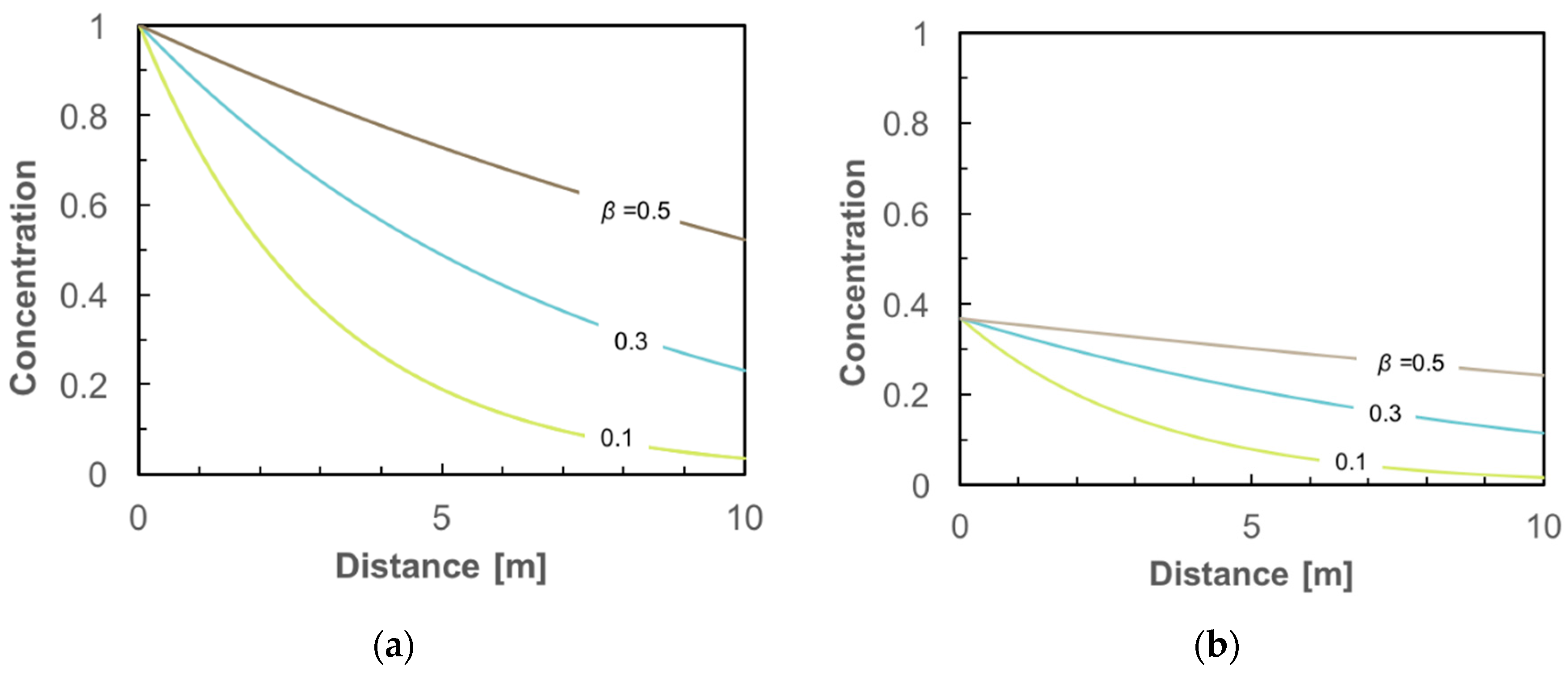
Figure 3.
Effects of beta on time history at with and . (a) Constant boundary source concentration and (b) time-dependent boundary source concentration.
Figure 3.
Effects of beta on time history at with and . (a) Constant boundary source concentration and (b) time-dependent boundary source concentration.
© 2018 by the authors. Licensee MDPI, Basel, Switzerland. This article is an open access article distributed under the terms and conditions of the Creative Commons Attribution (CC BY) license (http://creativecommons.org/licenses/by/4.0/).
Share and Cite
MDPI and ACS Style
Suzuki, A.; Fomin, S.; Chugunov, V.; Hashida, T. Mathematical Modeling of Non-Fickian Diffusional Mass Exchange of Radioactive Contaminants in Geological Disposal Formations. Water 2018, 10, 123. https://doi.org/10.3390/w10020123
AMA Style
Suzuki A, Fomin S, Chugunov V, Hashida T. Mathematical Modeling of Non-Fickian Diffusional Mass Exchange of Radioactive Contaminants in Geological Disposal Formations. Water. 2018; 10(2):123. https://doi.org/10.3390/w10020123
Chicago/Turabian StyleSuzuki, Anna, Sergei Fomin, Vladimir Chugunov, and Toshiyuki Hashida. 2018. "Mathematical Modeling of Non-Fickian Diffusional Mass Exchange of Radioactive Contaminants in Geological Disposal Formations" Water 10, no. 2: 123. https://doi.org/10.3390/w10020123
Note that from the first issue of 2016, this journal uses article numbers instead of page numbers. See further details here.