3-D Numerical Investigation on Oxygen Transfer in a Horizontal Venturi Flow with Two Holes

Abstract

In order to investigate the dissolved oxygen increase caused by air suction in a horizontal Venturi flow with two holes, a 3-D computational fluid dynamics model was used to explore the water and bubble mixture flow, coupled with a dissolved oxygen transfer model. A series of experiments were conducted to validate the mathematical model. A relative saturation coefficient correlation was examined factoring in dissolved oxygen concentration at the inlet, water velocity at the inlet, the hole’s diameter, contraction ratio at throat section, and the downstream length of Venturi pipe. It was found that the relative saturation coefficient increases with increasing dissolved oxygen concentration at the inlet and downstream length of Venturi pipe respectively. However, it increases with decreasing water velocity at the inlet and contraction ratio at the throat section to some extent. The hole’s diameter plays a complex role in the relative saturation coefficient. The dimensional analysis method and the least square method were used to deduce a simple formula for the relative saturation coefficient, and this was consistent with related data.

1. Introduction

Dissolved oxygen (DO) concentration is an important water quality index. A lower value usually causes a serious environmental issue for a body of water, including decreasing the capacity of creatures living within it to grow, reproduce, and survive [1]. To improve DO concentration in lakes and rivers and prevent water quality deterioration, aeration is commonly used [2,3,4]. As a simple device, the Venturi meter is widely applied in industrial applications to control the flow rate of fluids. The flow characteristics and pressure drop of a gas–coal mixture through the Venturi under high pressure was investigated experimentally [5]. The upstream and downstream pressure effects of Venturi flow were studied in terms of the flow rate and critical pressure ratio, both experimentally and numerically. Geometrical parameters such as the throat diameter, throat length, and diffuser angle were also considered [6]. The pressure drops between different sections have also been measured and analyzed for a two-phase flow of Venturi, as in the case of a typical nuclear accident [7]. A series of Venturi cavitation experiments were conducted with various upstream, throat and downstream lengths, and a model for water vapor void fraction was proposed to investigate the cavitating process [8]. He and Bai [9] found that the k-ε model was in agreement with experimental data on wet gas flow in the Venturi meter. Due to the water quality improvement caused by aeration, by using a Venturi flow with holes, the aeration coefficient relationship was examined and found to be well within the geometrical parameters experimentally and numerically [10,11,12].

The aforementioned hydraulic characteristic of a Venturi flow has been investigated extensively. However, a thorough understanding of the DO variation of a Venturi flow with air bubbles is still lacking. The objective of this research was to evaluate DO variation in an air-water two-phase flow through a horizontal Venturi pipe with two holes (HVFTH), experimentally and numerically. In addition, the relative saturation coefficient relationship with the hydraulic parameters and geometrical parameters of the Venturi pipe was investigated. Furthermore, a simple formula for the relative saturation coefficient was developed with the dimensional analysis method and the least square method.

2. Materials and Methods

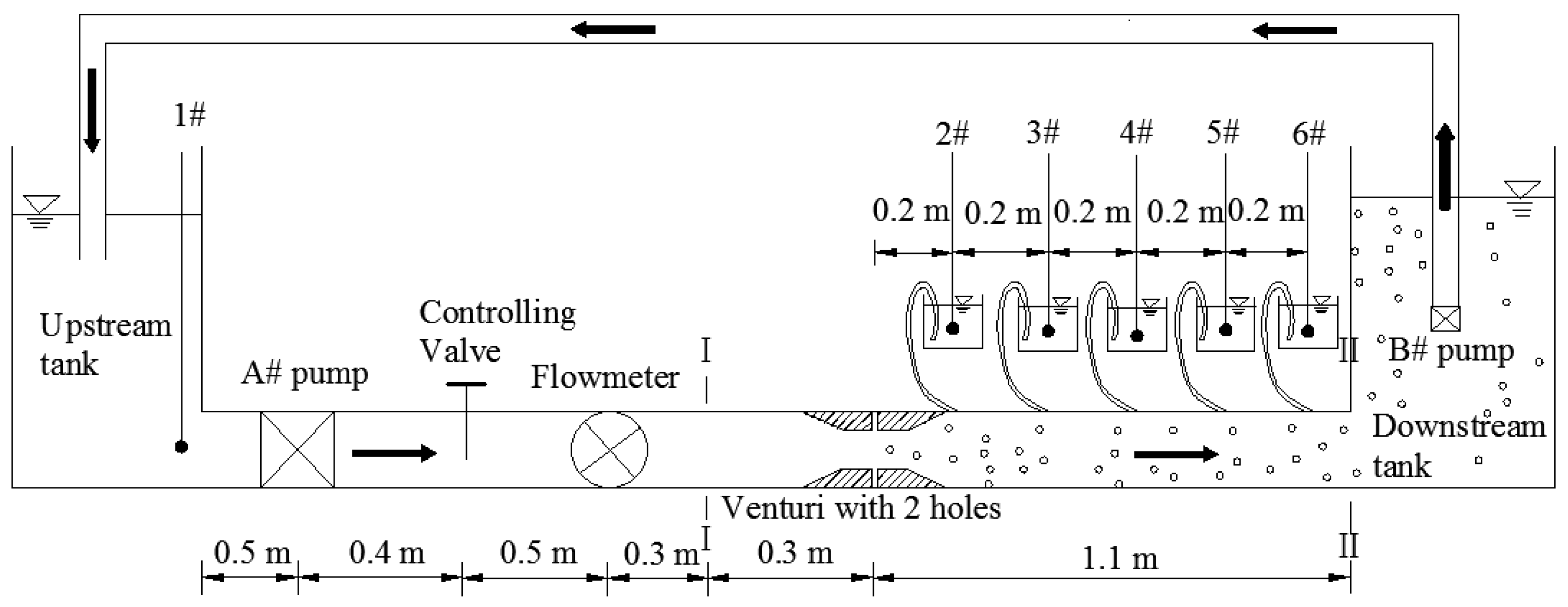
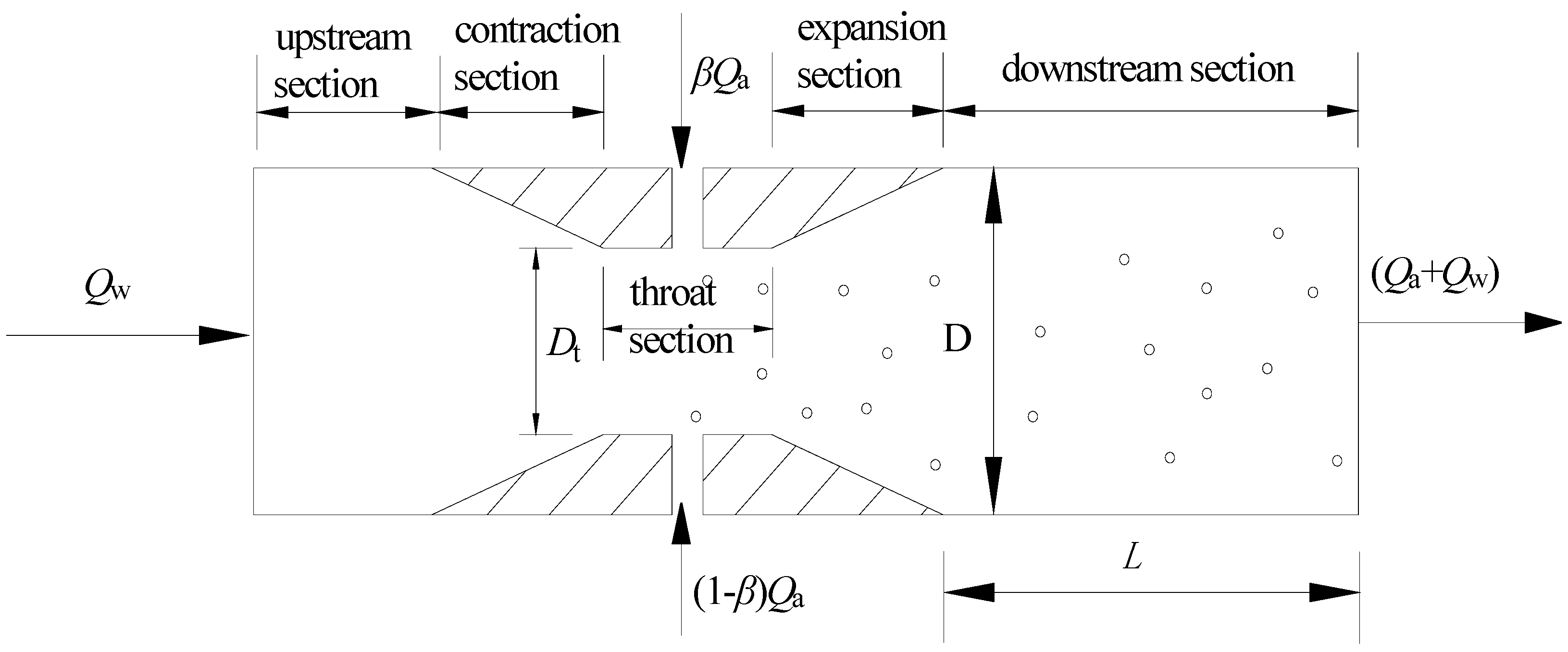
2.1. Experimental Setup and Instrumentation

In order to examine the DO variation for HVFTH, a series of experiments were conducted in the Hydraulic Lab at Ocean University of China. Figure 1 shows that the Venturi pipe with two holes consists of an upstream section, a contraction section, a throat section, an expansion section, and a downstream section. At the throat section, two suction holes are drilled through its upper wall and bottom wall, respectively. A PVC circular horizontal pipe with an inner diameter D of 0.021 m and a length of 3.1 m was used to connect two cylindrical water tanks, as shown in Figure 2. The diameter and height for both tanks are 0.58 m and 0.73 m, respectively. Water flowed from the upstream tank to the downstream tank via the A# water pump located 0.5 m downstream of the pipe inlet, and then it was pumped back to the upstream tank by the B# water pump in the downstream tank. The water flow rate in the pipe was controlled by a controlling valve located 0.4 m downstream of the A# water pump. The water velocity inside the pipe was measured using an electromagnetic flowmeter located 0.5 m downstream of the controlling valve. The Venturi pipe with two holes was fixed 0.6 m downstream of the flowmeter, and the center of the holes is defined as zero location in the longitudinal x-direction. The throat diameter of Venturi pipe, D_t, is 0.005 m, and the two circular holes’ diameters, d, are both 0.0007 m. Six DO probes numbered 1# to 6#, as shown in Figure 2, were used to measure the DO concentrations and water temperatures, where 1# DO probe was fixed in the upstream tank. Note that it is arduous to insert the other five DO probes into the PVC pipe to investigate the DO concentration variations, due to the undersized diameter of pipe. In order to solve this problem, five thin connection tubes were inserted into the downstream section with a spacing of 0.2 m between each tube. Five glass cups were used to collect the water through the five connection tubes. The 2# to 6# DO probes were submerged in the corresponding cups, and were used to measure the DO concentrations. In particular, the 2# to 6# DO probes approach the connection tube outlets as far as possible to ensure measurement accuracy and avoid the effect of oxygen transfer on the water surface. The corresponding DO concentrations were regarded as the values at the sections of five connection tubes without causing major deviations.

2.2. Experimental Procedure and Phenomena

Before the start of each experiment, the two tanks were filled with fresh tap water to 75% of the tanks’ height. It was well known that anhydrous sodium sulfite (Na₂SO₃) is capable of scavenging DO effectively and has long been used in the presence of a catalyst (CoCl₂) to scavenge DO in water [13]. According to the chemical Equation (1), the suitable weight of Na₂SO₃ was determined by considering the water volume in the system, the present DO concentration, and its desired value. The amount of CoCl₂ was suggested to be about 0.1% of Na₂SO₃ by weight [13,14]. Na₂SO₃ and CoCl₂ were put into the two water tanks as uniformly as possible. The water pumps then started to transport the water between the two tanks while mixing the water, Na₂SO₃ and CoCl₂ effectively. The controlling valve was used to control the water flow rate so as to ensure air suction through the two holes at the Venturi pipe, and the water flow rate was measured by the flowmeter. The DO concentrations were measured and recorded once per minute by six DO probes. In order to avoid a possible deviation due to the incomplete reaction between Na₂SO₃ and DO, DO concentration data were not used until it increased steadily.

$$2{\mathrm{Na}}_2{\mathrm{SO}}_3+{\mathrm{O}}_2\stackrel{{\mathrm{CoCl}}_2}{\to }2{\mathrm{Na}}_2{\mathrm{SO}}_4$$

(1)

The experiment shows that the outside gas moves into the Venturi pipe through the two holes due to the inside and outside pressure difference, and a large number of air bubbles are produced. At the throat section and expansion section, a strong bubbly collision, coalescence and breakup occurs because of the water turbulence and shearing force, and the bubbles are distributed widely. When the water and bubble mixture flows into the downstream section, the buoyancy effect strengthens, the bubbles begin to ascend to some extent, and some bubbles swarm to collide with the upper wall. At the end of the downstream section, the water and bubble mixture is injected into the downstream tank, an inverse flow appears with a counter-clockwise direction vortex, and the bubbles ascend to escape from the water surface in the downstream tank. In terms of the DO concentration variations measured by 2# to 6# DO probes, they increase successively, confirming the ability to enhance the DO concentrations by using a HVFTH.

2.3. Governing Equations

Concerning the mathematical model to investigate the turbulence of water and the air bubbles’ two-phases, considerable attention has been devoted to discussing their coupling effect. Euler–Euler methods consider the water and the bubbles as a pseudo-continuum and an averaging procedure is applied to both of them [15,16]. Euler–Lagrange methods represent only the water motion through the Navier–Stokes equations, while the bubbly motion is obtained by the direct solution of its trajectory using Newton’s second law [15]. Torti [15] used the Eulerian–Lagrangian one-way coupling method to evaluate the water and the bubbly convection separately, where the bubbles were simply considered to be carried by the water and the bubbly effect they had on the water was negligible. However, the algebraic slip mixture model does not assume that there is an interface between these two immiscible phases, and it allows the two phases to interpenetrate as well as move at different velocities [12]. Consequently, it was used to model the water and air bubbles’ motion in HVFTH, due mainly to its good simplification and computational accuracy. The continuity equation can be expressed as Equation (2).

$$\frac{\partial {\rho }_{\mathrm{m}}}{\partial t}+\frac{\partial \left({\rho }_{\mathrm{m}}{u}_{\mathrm{mi}}\right)}{\partial x_{\mathrm{i}}}=0$$

(2)

where t is time, x_i is the coordinate in i direction. For i = 1, 2, 3, x_i is x, y and z, respectively. The mixture density ρ_m and the mixture velocity $u_{\mathrm{mi}}$ in i direction can be defined as Equations (3) and (4).

$${\rho }_{\mathrm{m}}={\displaystyle \sum _{n=1}^2{\alpha }_{\mathrm{n}}}{\rho }_{\mathrm{n}}$$

(3)

$$u_{\mathrm{m}i}=\frac{1}{{\rho }_{\mathrm{m}}}{\displaystyle \sum _{n=1}^2{\alpha }_{\mathrm{n}}}{\rho }_{\mathrm{n}}{u}_{\mathrm{ni}}$$

(4)

where α_n, ρ_n, and u_ni are the volume fraction, the density and the i direction velocity of the n-phase, respectively. n = 1 represents the air phase, and n = 2 represents the water phase.

Its momentum equation was expressed as Equation (5).

$$\frac{\partial }{\partial t}({\rho }_{\mathrm{m}}{u}_{\mathrm{mj}})+\frac{\partial ({\rho }_{\mathrm{m}}{u}_{\mathrm{mi}}{u}_{\mathrm{mj}})}{\partial x_{\mathrm{i}}}=-\frac{\partial p_{\mathrm{m}}}{\partial x_{\mathrm{j}}}+\frac{\partial }{\partial x_{\mathrm{i}}}\left[{\mu }_{\mathrm{m}}\left(\frac{\partial u_{\mathrm{mi}}}{\partial x_{\mathrm{j}}}+\frac{\partial u_{\mathrm{mj}}}{\partial x_{\mathrm{i}}}\right)\right]+{\rho }_{\mathrm{m}}g+\nabla \cdot \left({\displaystyle \sum _{n=1}^2{\alpha }_{\mathrm{n}}{\rho }_{\mathrm{n}}{u}_{\mathrm{dr},\mathrm{n}}{u}_{\mathrm{dr},\mathrm{n}}}\right)$$

(5)

where μ_m is the dynamic viscosity of the water and air bubble mixture, ${\mu }_{\mathrm{m}}={\displaystyle \sum _{n=1}^2{\alpha }_{\mathrm{n}}}{\mu }_{\mathrm{n}}$, μ₁ and μ₂ are the dynamic viscosities of air bubbles and water, respectively. g is the gravitational acceleration. p_m is the mixture pressure. u_dr,n is the diffusion velocity of the n-phase and it can be expressed as Equation (6). The diffusion velocity of a phase is usually caused by density differences, which results in forces on the bubbles differing from those on water:

$$u_{\mathrm{dr},\mathrm{n}}=u_{\mathrm{qn}}-{\displaystyle \sum _{n=1}^2\frac{{\alpha }_{\mathrm{n}}{\rho }_{\mathrm{n}}}{{\rho }_{\mathrm{m}}}}{u}_{\mathrm{qn}}$$

(6)

$$u_{\mathrm{qn}}=\frac{\left({\rho }_{\mathrm{n}}-{\rho }_{\mathrm{m}}\right)d_{\mathrm{b}}^2}{18{\mu }_{\mathrm{eff}}{f}_{\mathrm{drag}}}\left[g-\left(u_{\mathrm{mi}}\cdot \nabla u_{\mathrm{mi}}\right)-\frac{\partial u_{\mathrm{mi}}}{\partial t}\right]$$

(7)

where $u_{\mathrm{qn}}$ is the slip velocity between two phases and it can be expressed as Equation (7); μ_eff is the effective viscosity; and d_b is the bubble diameter. The drag function f_drag can be defined as Equation (8).

$$f_{\mathrm{drag}}=\{\begin{array}{cc}1+0.15{\mathrm{Re}}_{\mathrm{b}}{}^{0.687}\hfill & \left({\mathrm{Re}}_{\mathrm{b}}\le 1000\right)\\ 0.0183{\mathrm{Re}}_{\mathrm{b}}\hfill & \left({\mathrm{Re}}_{\mathrm{b}}>1000\right)\end{array}$$

(8)

where Re_b is the bubble Reynolds number.

The air volume fraction equation was used to predict the air volume evolution as Equation (9).

$$\frac{\partial }{\partial t}({\alpha }_1{\rho }_1)+\nabla \cdot ({\alpha }_1{\rho }_1{u}_{\mathrm{mi}})=0$$

(9)

The Renormalization Group (RNG) k-ε model derived by [17] was used to investigate the air-water turbulence due to a satisfactory capacity to model the complex boundary flow considering the buoyancy effect. The turbulent kinetic energy, k, equation was written as Equation (10).

$$\frac{\partial }{\partial t}({\rho }_{\mathrm{m}}k)+\frac{\partial }{\partial x_{\mathrm{i}}}({\rho }_{\mathrm{m}}k{u}_{\mathrm{mi}})=\frac{\partial }{\partial x_{\mathrm{j}}}\left({\beta }_{\mathrm{k}}{\mu }_{\mathrm{eff}}\frac{\partial k}{\partial x_{\mathrm{j}}}\right)+G_{\mathrm{k}}-{\rho }_{\mathrm{m}}\epsilon$$

(10)

The turbulent dissipation rate, ε, equation was expressed as Equation (11).

$$\frac{\partial }{\partial t}\left({\rho }_{\mathrm{m}}\epsilon \right)+\frac{\partial }{\partial x_{\mathrm{i}}}\left({\rho }_{\mathrm{m}}\epsilon u_{\mathrm{mi}}\right)=\frac{\partial }{\partial x_{\mathrm{j}}}\left({\beta }_{\mathsf{\epsilon }}{\mu }_{\mathrm{eff}}\frac{\partial \epsilon }{\partial x_{\mathrm{j}}}\right)+C_{1\mathsf{\epsilon }}\frac{\epsilon }{k}{G}_{\mathrm{k}}-C_{2\mathsf{\epsilon }}{\rho }_{\mathrm{m}}\frac{{\epsilon }^2}{k}$$

(11)

where G_k represents the generation of turbulent kinetic energy caused by the average velocity, $G_{\mathrm{k}}=-{\rho }_{\mathrm{m}}{u}_{\mathrm{i}}{u}_{\mathrm{j}}\frac{\partial u_{\mathrm{j}}}{\partial x_{\mathrm{i}}}$; ${\mu }_{\mathrm{eff}}={\mu }_{\mathrm{m}}+{\mu }_{\mathrm{t}}$, μ_t is the turbulent eddy viscosity, ${\mu }_{\mathrm{t}}={\rho }_{\mathrm{m}}{C}_{\mathsf{\mu }}\frac{k^2}{\epsilon }$, C_μ = 0.0845. The value of C_μ is very close to the empirically-determined value of 0.09 used in the standard k-ε model; Pr_t is the turbulence Prandtl number, Pr_t = 0.07179. ${\beta }_{\mathrm{k}}$ and ${\beta }_{\mathsf{\epsilon }}$ are the inverse effective Prandtl numbers for k and ε, respectively. $C_{1\mathsf{\epsilon }}$ = 1.42 and $C_{2\mathsf{\epsilon }}$ = 1.68. Note that although these constants are simple, they have a wide range of applications with commendable accuracy [17,18].

The DO transfer equation was utilized to compute the DO concentration variation, and it was denoted as Equation (12) [19,20].

$$\frac{\partial \left({\rho }_{\mathrm{m}}C\right)}{\partial t}+\frac{\partial \left({\rho }_{\mathrm{m}}{u}_{\mathrm{mi}}C\right)}{\partial x_{\mathrm{i}}}=\frac{{\partial }^2\left({\Gamma }_{\mathrm{c}}C\right)}{\partial x_{\mathrm{i}}^2}+{\rho }_{\mathrm{m}}{S}_{\mathrm{c}}$$

(12)

where C is the DO concentration; Γ_C is the turbulent diffusion coefficient, Γ_C = ρ_mν_t/σ_t, where ν_t is turbulent viscosity, and σ_t is turbulent Schmidt number, where σ_t = 0.7. S_c is the source term representing the oxygen mass transfer across the interface between the water and bubbles, and it can be modeled as Equation (13) [21].

$$S_{\mathrm{c}}=K_{\mathrm{L},\mathrm{B}}{a}_{\mathrm{B}}(C_{\mathrm{s}}-C)$$

(13)

where K_L,Ba_B is the bubble transfer coefficient, K_L,B is the liquid film mass transfer coefficient, and a_B is the specific interfacial area of the bubbles defined as the contact area with water per unit volume of air-water mixture, and it can be expressed as a_B = 3α₁/d_b. d_b is the air bubble diameter with the assumption of a spherical shape, and it can be expressed as Equation (14) [22].

$$d_{\mathrm{b}}=1.5g^{-0.44}{\sigma }^{0.34}{\mu }_2^{0.22}{\rho }_2^{-0.45}{\rho }_1^{-0.11}{U}_1^{-0.02}$$

(14)

where σ is the surface tension, and U₁ is the superficial air velocity. The expression of d_b is relatively simple; however, it was found to work well in a number of studies [23,24]. C_s is the saturation DO concentration, related to water temperature and pressure [25].

In this study, K_L,B is calculated as the maximum value between bubbles rising in stagnant liquid [26] and bubbles in turbulent flow [27], and it can be expressed as Equation (15).

$$K_{\mathrm{L},\mathrm{B}}=\max \left\{0.4{\left(\frac{{\nu }_{\mathrm{m}}}{D_{\mathrm{m}}}\right)}^{-0.5}{\left({\nu }_{\mathrm{m}}\epsilon \right)}^{0.25},\frac{D_{\mathrm{m}}{\mathrm{Pe}}^{0.5}}{d_{\mathrm{b}}\sqrt{\pi }}\left[1-\frac{2}{3}{\left(1+0.09{\mathrm{Re}}_{\mathrm{b}}^{\frac{2}{3}}\right)}^{-\frac{3}{4}}\right]\right\}$$

(15)

where D_m is the oxygen molecular diffusion coefficient related to temperature [25], $v_{\mathrm{m}}={\displaystyle \sum _{n=1}^2{\alpha }_{\mathrm{n}}}{v}_{\mathrm{n}}$, ν_m, ν₁ and ν₂ are the kinematic viscosity coefficients of mixture, air bubbles and water, respectively. P_e is the Peclet number.

2.4. Initial and Boundary Conditions

The two sections of I-I and II-II, as shown in Figure 2, were regarded as the inlet and outlet boundaries in the mathematical model, and the computational domain was set from section I-I to section II-II. At the I-I section boundary, the water velocity measured by the flowmeter and DO concentration measured by 1# DO probe were used as the desired values respectively, and the turbulent parameters k and ε were determined approximately using Equations (16) and (17).

$$k=\frac{3}{2}{\left(U_{\mathrm{in}}I\right)}^2$$

(16)

$$\epsilon =C_{\mathsf{\mu }}^{0.75}\frac{k^{1.5}}{l}$$

(17)

where U_in is the average velocity at I-I cross section, I is the turbulence intensity, and l is the turbulence length scale. In addition, l is a physical quantity related to the size of the large eddies that contains the energy in turbulent flows. In fully-developed pipe flows, l is restricted by the size of the pipe, since the turbulent eddies cannot be larger than the pipe size. An approximate relationship between l and the physical size of the pipe is expressed as Equation (18).

$$l=\frac{0.07D}{C_{\mathsf{\mu }}^{3/4}}$$

(18)

where the factor of 0.07 is based on the maximum value of the mixing length in fully-developed turbulent pipe flow.

At the II-II section boundary fully developed turbulence was assumed, and the variation ratios for all the variables were set as 0. At the two holes boundaries, the atmosphere pressure was assumed, and the DO concentration was set as the same value as at the I-I section without high deviation.

2.5. Numerical Details

The CFD solver Fluent 16.0 was utilized to solve the governing equations. The Finite Volume Method was used to discretize the governing equations. Pressure, turbulent kinetic energy, turbulent dissipation rate, air volume fraction, and DO concentration are set at the middle point of the cell. The velocity components were set at the cell edges. The convection term was solved with QUICK scheme, the diffusion term was solved with central scheme, and the SIMPLEC algorithm was used to couple pressure and velocity. In FLUENT 16.0 software, the User-Defined Scalar (UDS) method reported by Yin et al. [20] was used to compute DO concentrations by compiling DEFINE_SOURCE and DEFINE_DIFFUSIVITY macros in the C language environment. In addition, the grid acceleration convergence techniques were used to achieve better convergence speed and accuracy.

Solidworks 2012 software (Dassault Systèmes SolidWorks Corporation, Waltham, MA, USA) was used to generate the 3-D geometric body, and the ICEM 14.5 software (ANSYS, Canonsburg, PA, USA) was utilized to partition the computational cells. The refined cells were used to partition the local domain near the two holes. The relatively coarse cells were used to partition the other domain. Grid independence was tested using the grid convergence index (GCI) method, which is an acceptable and recommended method that has been evaluated in over several hundred CFD cases [28,29,30,31].

Table 1. Analysis of discretization error.

Grid		At the Centre of the 2 Holes Cross Section for Qw = 2.05 × 10−4 m3/s and Cin = 5 × 10−4 kg/m3
Grid Partition Scheme	Total Cells Number	Refined Cells Number	Water Velocity
Grid 1	3,640,723	1,383,413	31.86 m/s
Grid 2	457,235	172,919	31.37 m/s
Grid 3	40,154	18,396	35.47 m/s
Extrapolated values		32.35 m/s
Extrapolated relative error		1.5%
Grid convergence index		1.9%

shows the discretization error for the water velocities at the centre point of the 2 holes cross section for water flow rate Q_w = 2.05 × 10⁻⁴ m³/s and DO concentration at the inlet C_in = 5 × 10⁻⁴ kg/m³. The extrapolated relative error and GCI are computed by Richardson extrapolation. In x, y and z directions, three cell sizes are used in the GCI calculations: 0.00007 m × 0.00015 m × 0.00017 m of Grid 1, 0.00014 m × 0.00031 m × 0.00033 m of Grid 2 and 0.00028 m × 0.00062 m × 0.00066 m of Grid 3, respectively. The total cells number and the refined cells number for Grid 1, Grid 2 and Grid 3 are shown in Table 1. It was found that the discretization error is very small at 1.9% between Grid 2 and Grid 1 with the increasing refined cells number from 172,919 to 1,383,413. Thus, the Grid 2 scheme is relatively independent of the computational results. Therefore, it was selected for the following computations after considering the balance between accuracy and computational speed.

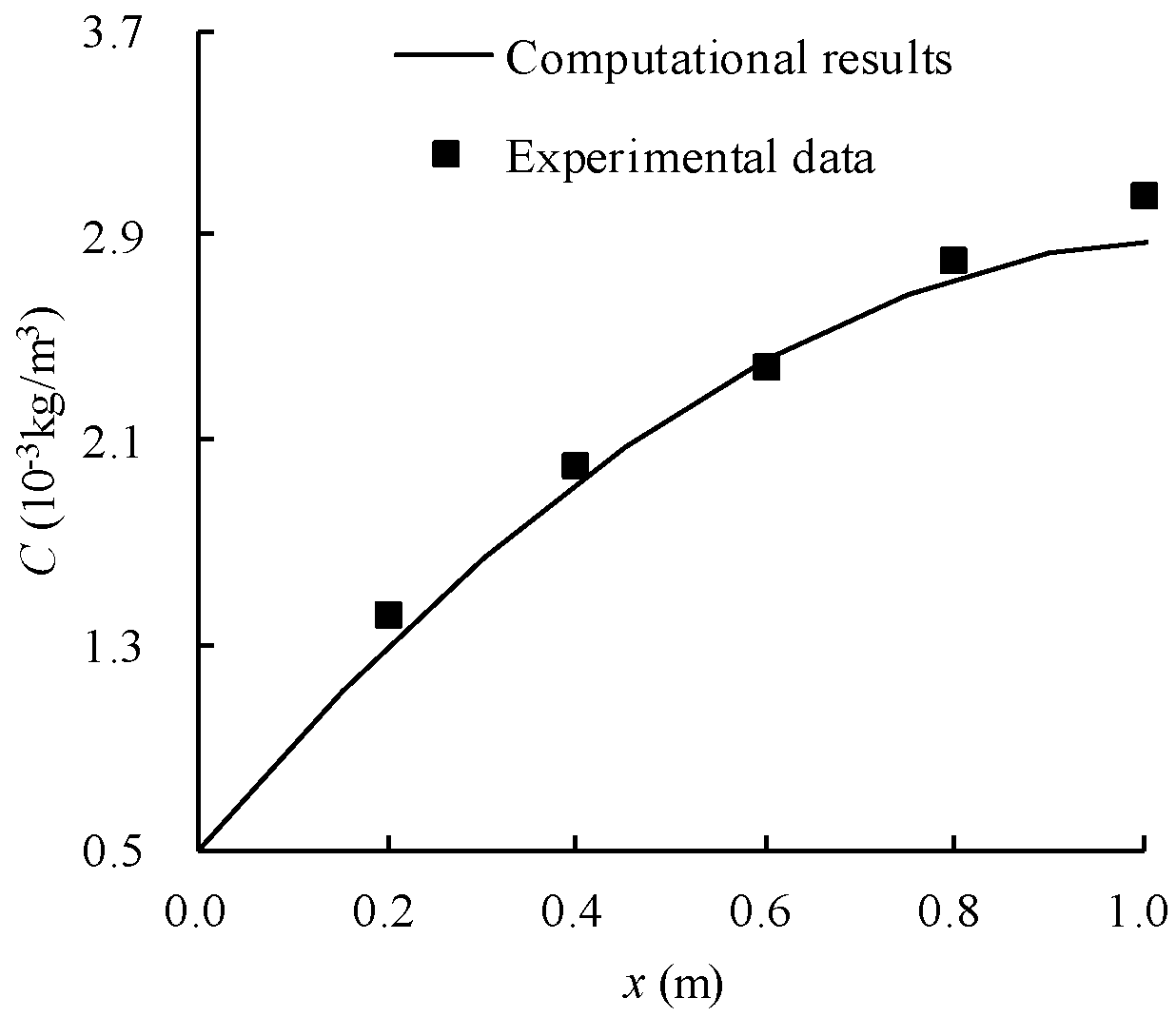
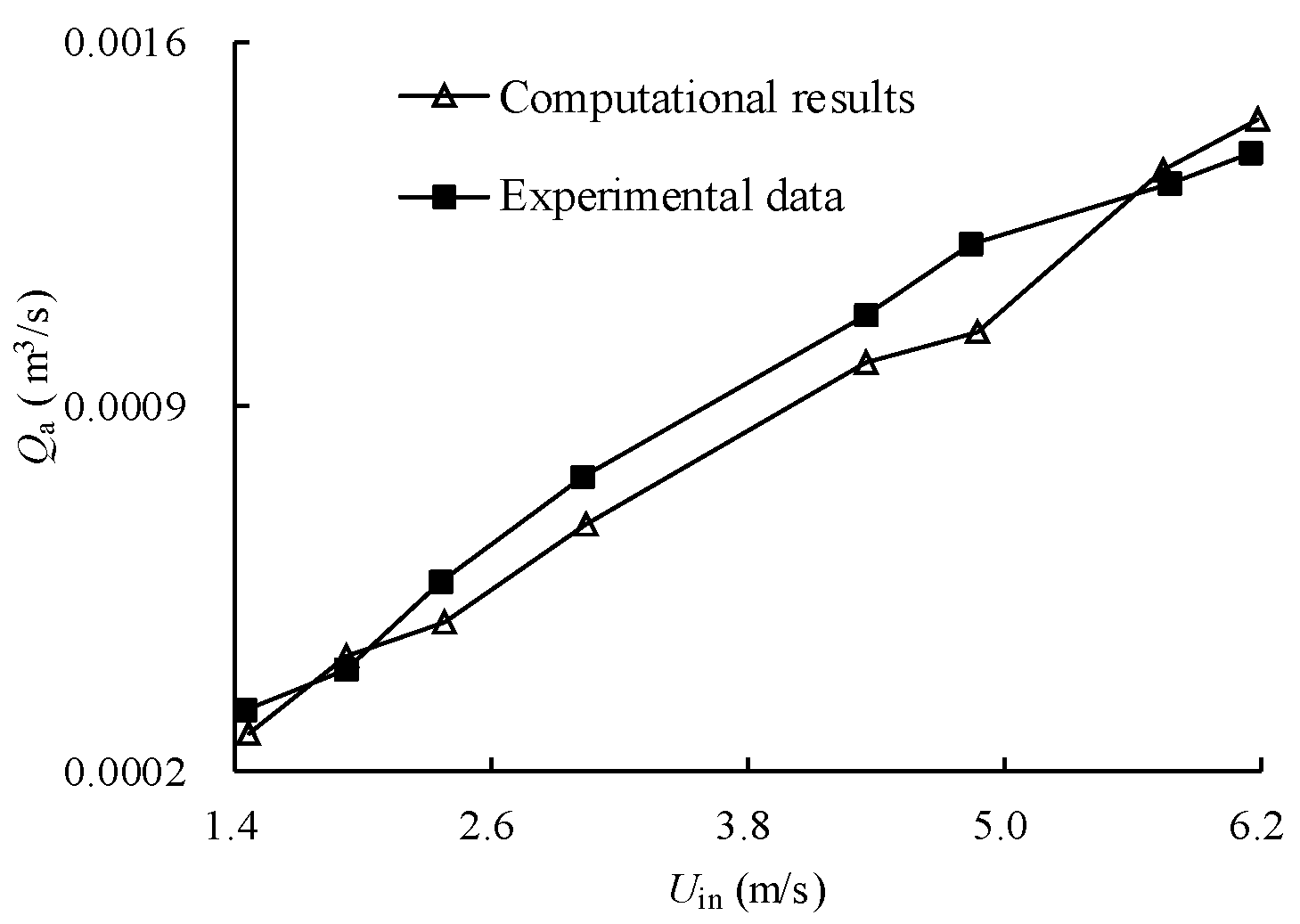
2.6. Model Validation

Figure 3 shows the computational DO concentrations and experimental data in the longitudinal direction for Q_w = 2.05 × 10⁻⁴ m³/s and C_in = 5 × 10⁻⁴ kg/m³. It was found that the maximum value of the relative deviation is 9.2% at the x = 0.2 m, while the other relative deviations are all smaller than 8%.

The proposed mathematical model was further validated on air flow rate Q_a using the experimental data reported by [12]. In the experiment by [12], D_t is 0.027 m, D is 0.036 m, d is 0.005 m, and the downstream section length, L, is 0.25 m. U_in was controlled at 1.47 m/s, 1.94 m/s, 2.37 m/s, 3.07 m/s, 4.35 m/s, 4.88 m/s, 5.76 m/s and 6.19 m/s respectively. Figure 4 shows the computational Q_a in comparison to experimental data. It was found that Q_a increases with increasing U_in. The relative deviations between experimental values and computational results are smaller than 10% in general, and are consistent with each other. Figure 3 and Figure 4 show that it is acceptable to predict the hydraulic parameters, such as C and Q_a, in a HVFTH using the proposed mathematical model.

3. Results and Discussion

265 scenarios of D = 0.2 m and T = 20 °C were simulated with: d increasing from 0.015 m to 0.020 m, 0.025 m, and 0.030 m; contraction ratio at the throat section (δ = D_t/D) increasing from 0.5 to 0.6, 0.7 and 0.8; L increasing from 2 m to 3 m; U_in increasing from 2.78 m/s to 6.5 m/s; and C_in increasing from 0 kg/m³ to 0.001 kg/m³, 0.002 kg/m³, 0.003 kg/m³, 0.004 kg/m³ and 0.005 kg/m³.

A relative saturation coefficient, E, is defined for analyzing DO recovery as Equation (19) [20].

$$E=\frac{C_{\mathrm{out}}-C_{\mathrm{in}}}{C_{\mathrm{s}}-C_{\mathrm{in}}}=1-e^{-k_{\mathrm{L},\mathrm{B}}{a}_{{}_{\mathrm{B}}}\Delta t}$$

(19)

where C_out is the average value of the DO concentration at section II-II, and Δt is the travel time from the two holes’ cross section to section II-II.

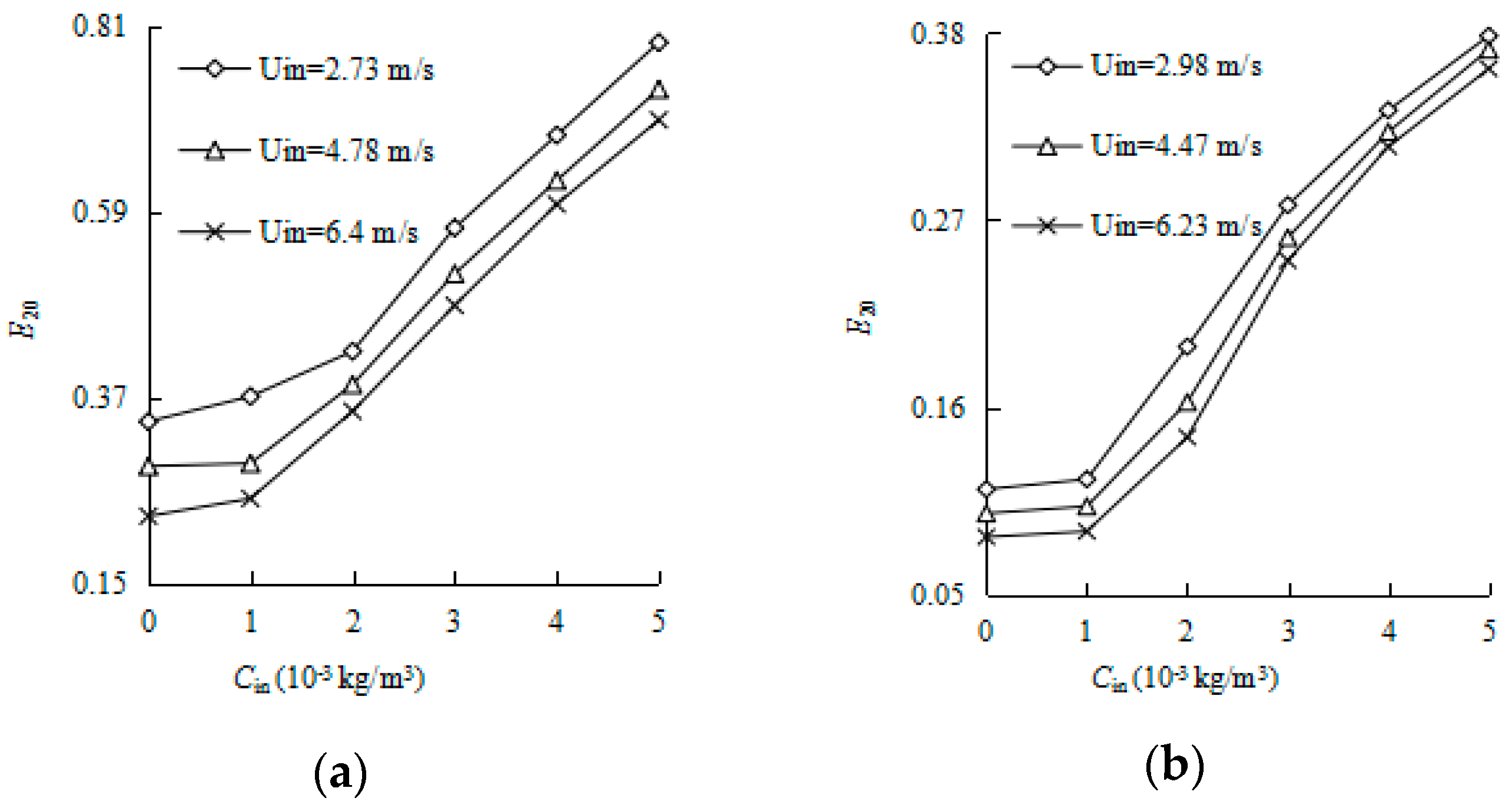
3.1. Effect of Hydraulic Parameters

Figure 5 shows the E₂₀ relationship with U_in for D = 0.2 m, L = 3 m and C_in = 0 kg/m³, where E₂₀ is the E value at 20 °C water temperature. It was found that E₂₀ decreases with increasing U_in. The possible reason is that as Δt decreases due to the increasing U_in, the bubbles flow faster in the Venturi pipe and oxygen has less time to transfer from air bubbles to the water body, resulting in the decrease of E₂₀ according to Equation (19). Therefore, U_in plays a significant role in E₂₀.

Figure 6 shows the E₂₀ relationship with C_in for D = 0.2 m, d = 0.02 m and L = 3 m. It was found that E₂₀ increases with increasing C_in. For a given C_s in hypoxic water, with the increasing C_in, C_out increases, $C_{\mathrm{s}}-C_{\mathrm{in}}$ decreases, and $C_{\mathrm{out}}-C_{\mathrm{s}}$ increases. Equation (19) can be rewritten as $E=1+\frac{C_{\mathrm{out}}-C_{\mathrm{s}}}{C_{\mathrm{s}}-C_{\mathrm{in}}}$, and it increases as a result. Therefore, C_in also plays an important role in E₂₀. In addition, it was interesting to note that E₂₀ sensitivity decreases with increasing C_in and δ.

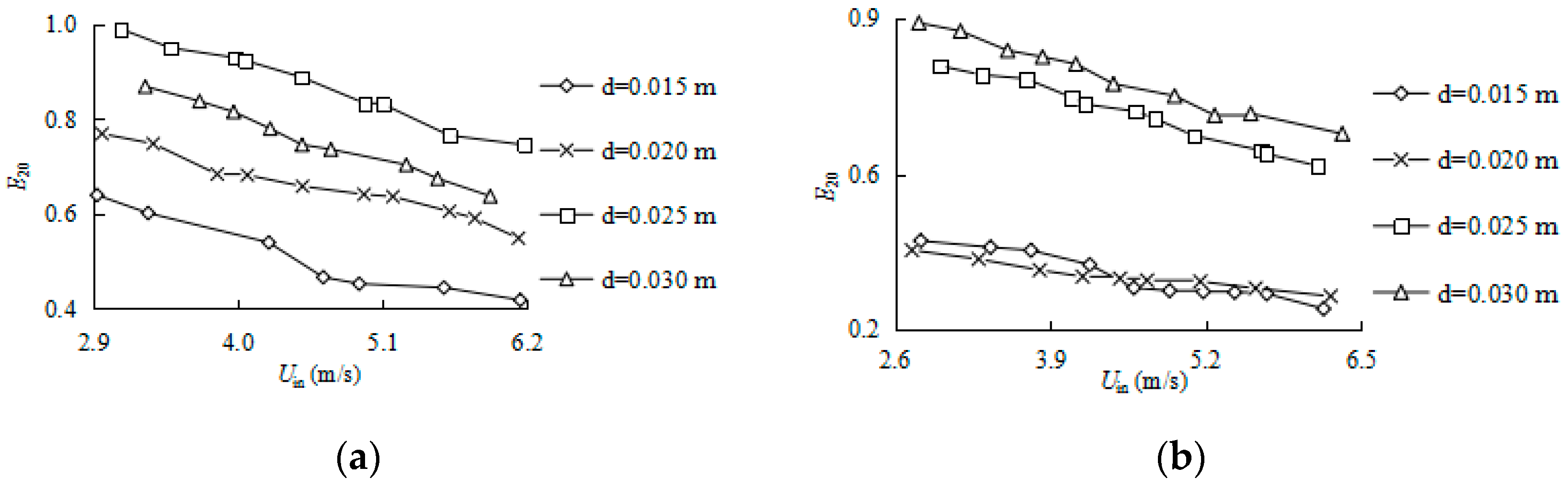
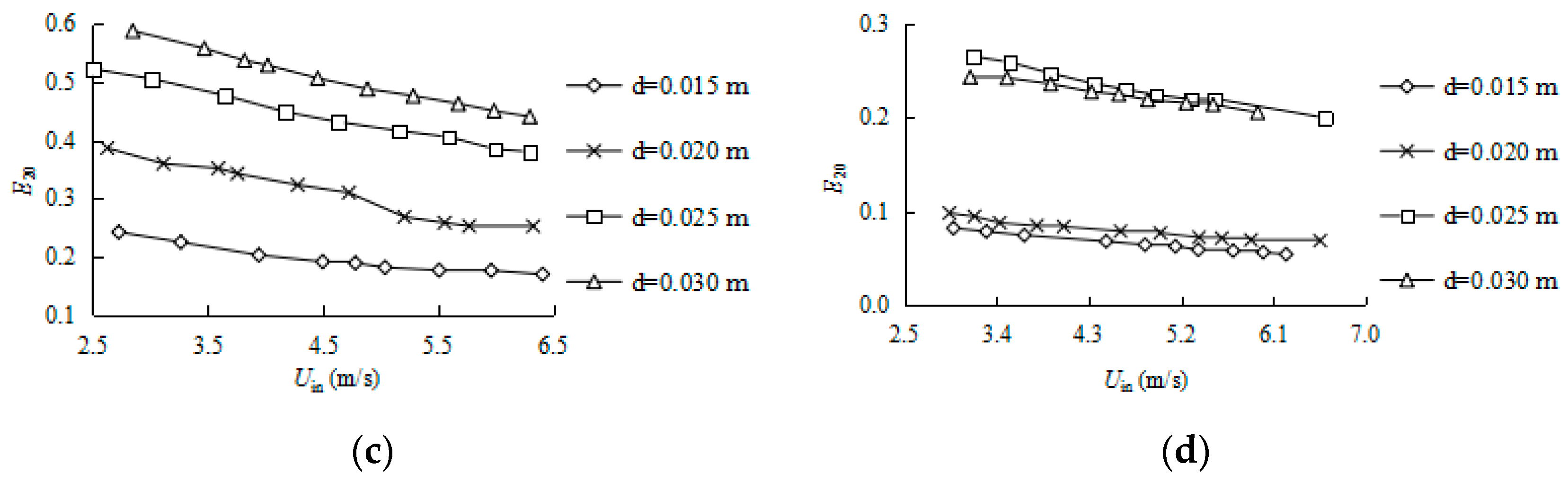
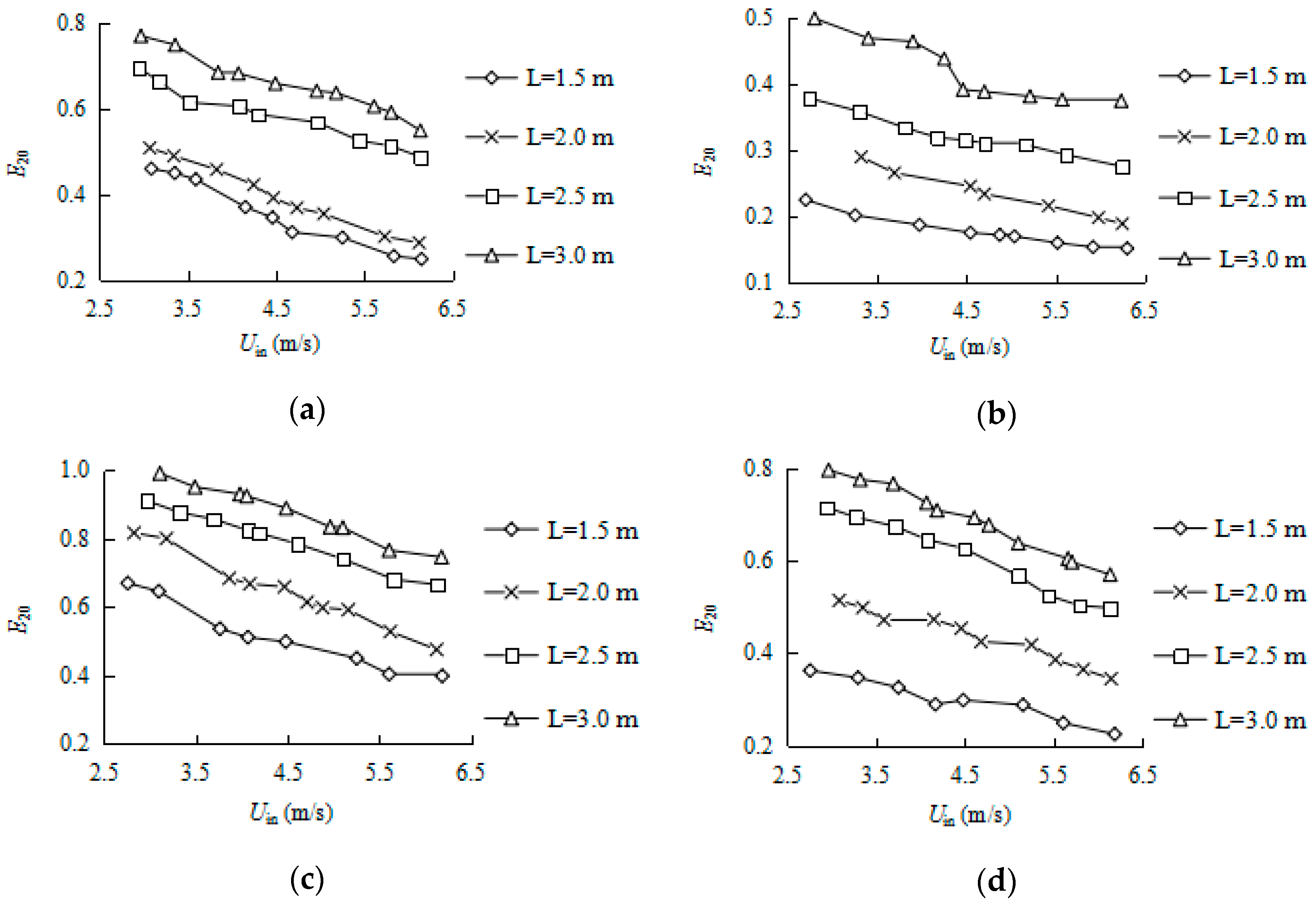
3.2. Effect of Geometric Parameters

Figure 7 shows that E₂₀ increases with increasing d to some extent, especially for small δ scenarios, and an optimum d exists corresponding to the maximum E₂₀. For large δ and d scenarios, E₂₀ does not increase much with the continual increase of d. Therefore, the diameter of the hole plays a complex role in E₂₀ and a simple comment on its effect is warranted. With a given water velocity at the inlet, the negative pressure usually occurs near the throat section of a conventional Venturi flow without hole(s). With the increase of the diameter of the holes from 0, the air flow rate through the holes increases, and the air volume fraction also increases, contributing to the increasing E₂₀. With the continual increase of the holes’ diameter, the increasing rate of Q_a slows due mainly to the negative pressure attenuation. In the case that the local pressure near the holes reaches the outside atmosphere pressure, the air suction phenomenon vanishes. With a large enough hole diameter, the local pressure becomes positive and the inside water will jet into the outside atmosphere through the holes, instead of air suction. Therefore, an optimum value of the diameter of the holes can be investigated for a given scenario. In addition, E₂₀ increases with decreasing δ as shown in Figure 7. A possible reason is that the negative pressure near the holes decreases due to the decreasing δ, and the air flow rate increases as a result, contributing to the increasing E₂₀. Furthermore, E₂₀ sensitivity attenuates in δ with the increase of the diameter of the holes.

Figure 8 shows that E₂₀ increases with increasing L for the scenarios of D = 0.2 m and C_in = 0 kg/m³. The reason is that with increasing L, Δt increases as a result, and it has more time to transfer oxygen from air bubbles to the water body, resulting in the increase of E₂₀ according to Equation (19). In addition, E₂₀ increases with increasing d and decreasing δ to some extent.

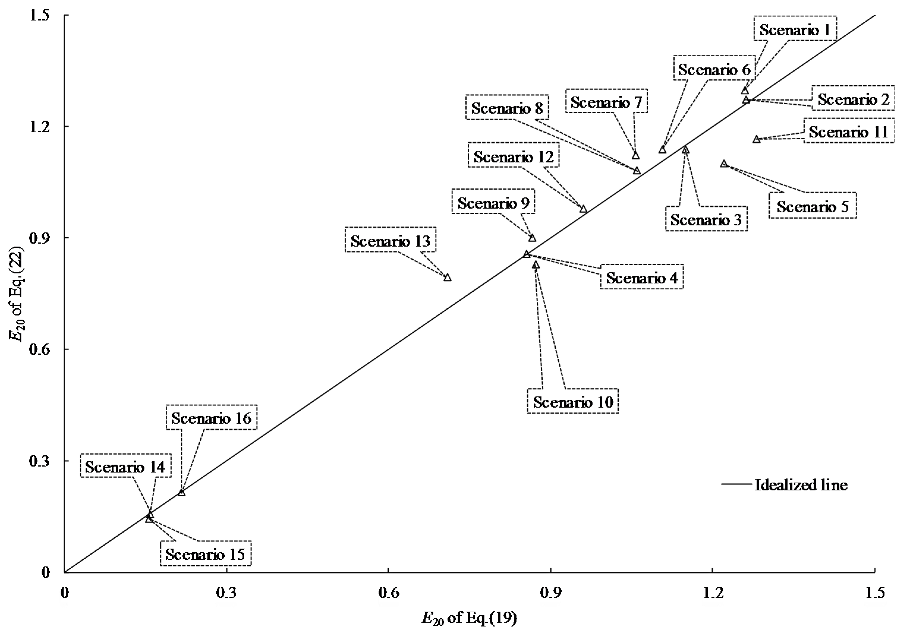
3.3. A Correlation for the Relative Saturation Coefficient

It is not easy to calculate the relative saturation coefficient by Equation (19), due to the difficulty determining k_L,Ba_B△t. Consequently, it is necessary to deduce a simple formula for the relative saturation coefficient considering the effects of D, D_t, d, L, U_in, C_in, C_s and ν₂, and E₂₀ can be written as Equation (20).

$$E_{20}=f\left(D_{\mathrm{t}},D,d,L,U_{\mathrm{in}},C_{\mathrm{in}},C_{\mathrm{s}},{\nu }_2\right)$$

(20)

Application of dimensional homogeneity to Equation (20) yields the Equation (21).

$$E_{20}=f\left(\delta ,d/D,L/D,\mathrm{Re},C_{\mathrm{in}}/C_{\mathrm{s}}\right)$$

(21)

where $\mathrm{Re}=U_{\mathrm{in}}D/{\nu }_2$. The 249 groups of numerical data from the aforementioned 265 scenarios were used randomly to deduce the following Equation (22) with the least squares method,

$$E_{20}=-1.59{\delta }^2+5.69\frac{d}{D}+0.052\frac{L}{D}+2.12\times {10}^{-8}\mathrm{Re}+0.56\frac{C_{\mathrm{in}}}{C_s}$$

(22)

The correlation coefficient is 0.88. In order to validate Equation (22), the other 16 scenarios were used as shown in

Table 2. 16 scenarios for validation with Equation (22) for D = 0.2 m.

Scenarios	Uin (m/s)	Cin (10−3 kg/m3)	d (m)	L (m)	δ
1	5.54	0	0.030	3	0.5
2	5.92	0	0.030	3	0.5
3	6.39	1	0.030	3	0.6
4	5.29	0	0.025	2	0.5
5	9.00	2	0.030	3	0.6
6	7.51	2	0.020	3	0.5
7	4.33	3	0.030	3	0.7
8	5.01	3	0.030	3	0.7
9	6.06	4	0.030	2	0.7
10	7.42	4	0.030	2	0.7
11	5.06	5	0.020	3	0.5
12	4.17	5	0.015	3	0.6
13	6.31	5	0.015	2	0.6
14	6.35	1	0.020	2	0.8
15	5.50	1	0.020	2	0.8
16	5.29	2	0.020	2	0.8

.

Figure 9 shows the E₂₀ validation between Equation (22) and the corresponding results yielded from Equation (19). It was found that they agree satisfactorily with each other; all the relative deviations between them are smaller than 20%, and most of them are smaller than 10%. Therefore, it is reliable to compute the relative saturation coefficient using Equation (22) without causing large deviations. Note that Equation (22) has good applicability to predict our results, while it still needs further validation for practical applications.

4. Conclusions

A 3-D two-phase flow mathematical model, coupled with a DO transfer model and a series of experiments, were conducted to investigate the DO recovery at a HVFTH. The computational DO concentration and air volume fraction were validated with experimental data, and they agree with each other well. In addition, the validated mathematical model was used to compute the hydraulic parameters, DO concentration and relative saturation coefficient within different scenarios. It was found that with increasing DO concentration at the inlet and downstream section length, the relative saturation coefficient increases. However, it decreases with the increase of water velocity at the inlet and throat section contraction ratio, respectively. The diameter of the holes plays a complex role in the relative saturation coefficient, and an optimum value may exist when the relative saturation coefficient reaches the maximum. The dimensional analysis method and the least square method were used to deduce a simple formula for the relative saturation coefficient considering the effect of geometric sizes and the hydraulic parameters, and it was validated well with the results of Equation (19).

References

1. Neilan, R.M.; Rose, K. Simulating the effects of fluctuating dissolved oxygen on growth, reproduction, and survival of fish and shrimp. J. Theor. Biol. 2014, 343, 54–68. [Google Scholar] [CrossRef] [PubMed]
2. Alp, E.; Melching, C.S. Allocation of supplementary aeration stations in the Chicago waterway system for dissolved oxygen improvement. J. Environ. Manag. 2011, 92, 1577–1583. [Google Scholar] [CrossRef] [PubMed]
3. McGinnis, D.F.; Lorke, A.; Wüest, A.; Stöckli, A.; Little, J.C. Interaction between a bubble plume and the near field in a stratified lake. Water Resour. Res. 2004, 40. [Google Scholar] [CrossRef]
4. Lima Neto, I.E.; Zhu, D.Z.; Rajaratnam, N.; Yu, T.; Spafford, M.; McEachern, P. Dissolved oxygen downstream of an effluent outfall in an Ice-Covered River: Natural and artificial aeration. J. Environ. Eng. ASCE 2007, 133, 1051–1060. [Google Scholar] [CrossRef]
5. Liu, K.; Lu, H.F.; Guo, X.L.; Sun, X.L.; Tao, S.H.; Gong, X. Experimental study on flow characteristics and pressure drop of gas-coal mixture through venture. Powder Technol. 2014, 268, 401–411. [Google Scholar] [CrossRef]
6. Ashrafizadeh, S.M.; Ghassemi, H. Experimental and numerical investigation on the performance of small-sized cavitating venturis. Flow Meas. Instrum. 2015, 42, 6–15. [Google Scholar] [CrossRef]
7. Monni, G.; Salve, M.E.; Panella, B. Two-phase flow measurements at high void fraction by a Venturi meter. Prog. Nucl. Energy 2014, 77, 167–175. [Google Scholar] [CrossRef]
8. Abdulaziz, A.M. Performance and image analysis of a cavitating process in a small type venture. Exp. Therm. Fluid Sci. 2014, 53, 40–48. [Google Scholar] [CrossRef]
9. He, D.J.; Bai, B.F. Numerical investigation of wet gas flow in Venturi meter. Flow Meas. Instrum. 2012, 28, 1–6. [Google Scholar] [CrossRef]
10. Baylar, A.; Ozkan, F. Applications of Venturi principle to water aeration systems. Environ. Fluid Mech. 2006, 6, 341–357. [Google Scholar] [CrossRef]
11. Baylar, A.; Ozkan, F.; Unsal, M. On the use of Venturi tubes in aeration. Clean-Soil Air Water 2007, 35, 183–185. [Google Scholar] [CrossRef]
12. Baylar, A.; Aydin, M.C.; Unsal, M.; Ozkan, F. Numerical modeling of Venturi flows for determining air injection rates using FLUENT V6.2. Math. Comput. Appl. 2009, 14, 97–108. [Google Scholar] [CrossRef]
13. Mantha, R.; Taylor, K.E.; Biswas, N.; Bewtra, J.K. A Continuous system for Fe0 reduction of nitrobenzene in synthetic waste water. Environ. Sci. Technol. 2001, 35, 3231–3236. [Google Scholar] [CrossRef] [PubMed]
14. Yin, Z.G.; David, Z.Z.; Liang, B.C.; Wang, L. Theoretical analysis and experimental study of oxygen transfer under regular and non-breaking waves. J. Hydrodyn. 2013, 25, 718–724. [Google Scholar] [CrossRef]
15. Torti, E.; Sibilla, S.; Raboni, M. An Eulerian-Lagrangian method for the simulation of the oxygen concentration dissolved by a two-phase turbulent jet system. Comput. Struct. 2013, 129, 207–217. [Google Scholar] [CrossRef]
16. Wörner, M. A Compact Introduction to the Numerical Modeling of Multi-Phase Flows; Institute für Reaktorsicherheit—Program Nuvkleare Sicherheitsfotschung; Springer: Berlin, Germany, 2003. [Google Scholar]
17. Yakhot, V.; Orszag, S.A. Renormalization-Group analysis of turbulence. Phys. Rev. Lett. 1986, 57, 1722. [Google Scholar] [CrossRef] [PubMed]
18. Chen, Q. Comparison of different k-ε models for indoor air flow computations. Numer. Heat Transf. B Fund. 1995, 28, 353–369. [Google Scholar] [CrossRef]
19. Faghri, A.; Zhang, Y.; Howell, J. Advanced Heat and Mass Transfer; Global Digital Press: Colombia, MO, USA, 2010. [Google Scholar]
20. Yin, Z.G.; Cheng, D.S.; Liang, B.C. Oxygen transfer by air injection in horizontal pipe flow. J. Environ. Eng. ASCE 2012, 139, 908–912. [Google Scholar] [CrossRef]
21. Geldert, D.A.; Gulliver, J.S.; Wilhelms, S.C. Modeling dissolved gas supersaturation below spillway plunge pools. J. Hydraul. Eng. ASCE 1998, 124, 513–521. [Google Scholar] [CrossRef]
22. Wilkinson, P.M.; Haringa, H.; Van Dierendonck, L.L. Mass transfer and bubble size in a bubble column under pressure. Chem. Eng. Sci. 1994, 49, 1417–1427. [Google Scholar] [CrossRef]
23. Rosso, D.; Larson, L.E.; Stenstrom, M.K. Surfactant effects on alpha factors in full-scale wastewater aeration systems. Water Sci. Technol. 2006, 54, 143–153. [Google Scholar] [CrossRef] [PubMed]
24. Laborde-Boutet, C.; Larachi, F.; Dromard, N.; Delsart, O.; Schweich, D. CFD simulation of bubble column flows: Investigations on turbulence models in RANS approach. Chem. Eng. Sci. 2009, 64, 4399–4413. [Google Scholar] [CrossRef]
25. Lide, D.R. CRC Handbook of Chemistry and Physics, 87th ed.; Internet Version; CRC Press/Taylor and Francis Group: Boca Raton, FL, USA, 2007. [Google Scholar]
26. Lamont, J.C.; Scott, D.S. An eddy cell model of mass transfer into the surface of a turbulent liquid. AIChE J. 1970, 16, 513–519. [Google Scholar] [CrossRef]
27. Politano, M.; Arenas Amado, A.; Bickford, S.; Murauskas, J.; Hay, D. Investigation into the total dissolved gas dynamics of wells dam using a two-phase flow model. J. Hydraul. Eng. 2010, 137, 1257–1268. [Google Scholar] [CrossRef]
28. Richardson, L.F.; Gaunt, J.A. The deferred approach to the limit. Part I. Single lattice. Part II. Interpenetrating lattices. Philos. Trans. R. Soc. Lond. Ser. A Contain. Pap. Math. Phys. Character 1927, 226, 299–361. [Google Scholar] [CrossRef]
29. Ferziger, J.H.; PERIĆ, M. Further discussion of numerical errors in CFD. Int. J. Numer. Methods Fluids 1996, 23, 1263–1274. [Google Scholar] [CrossRef]
30. Broadhead, B.L.; Rearden, B.T.; Hopper, C.M.; Wagschal, J.J.; Parks, C.V. Sensitivity-and uncertainty-based criticality safety validation techniques. Nucl. Sci. Eng. 2004, 146, 340–366. [Google Scholar] [CrossRef]
31. Celik, I.B.; Ghia, U.; Roache, P.J. Procedure for estimation and reporting of uncertainty due to discretization in CFD applications. J. Fluids Eng. 2008, 130, 078001. [Google Scholar]
Figure 1. Schematic of HVFTH.
Water 10 00174 g001
Figure 2. Experimental setup.
Water 10 00174 g002
Figure 3. Measured DO concentrations and predicted data in the longitudinal direction.
Water 10 00174 g003
Figure 4. Computational Qa and experimental data of [12].
Water 10 00174 g004
Figure 5. Effect of Uin on E20 (D = 0.2 m, L = 3 m and Cin = 0 kg/m3). (a) δ = 0.5; (b) δ = 0.6; (c) δ = 0.7; (d) δ = 0.8.
Water 10 00174 g005aWater 10 00174 g005b
Figure 6. Effect of Cin on E20 (D = 0.2 m, d = 0.02 m and L = 3 m). (a) δ = 0.7, (b) δ = 0.8.
Water 10 00174 g006
Figure 7. Effect of δ on E20 (D = 0.2 m, L = 3 m and Cin = 0 kg/m3). (a) d = 0.015 m; (b) d = 0.020 m; (c) d = 0.025 m; (d) d = 0.030 m.
Water 10 00174 g007
Figure 8. Effect of L on E20 (D = 0.2 m and Cin = 0 kg/m3). (a) δ = 0.5, d = 0.020 m; (b) δ = 0.6, d = 0.020 m; (c) δ = 0.5, d = 0.025 m; (d) δ = 0.6, d = 0.025 m.
Water 10 00174 g008
Figure 9. E20 using Equations (19) and (22).
Water 10 00174 g009