Article

Comparison of Precipitation and Streamflow Correcting for Ensemble Streamflow Forecasts

1
State Key Laboratory of Hydro-science and Engineering, Department of Hydraulic Engineering, Tsinghua University, Beijing 100084, China
2
State Key Laboratory of Simulation and Regulation of Water Cycles in River Basin, China Institute of Water Resources and Hydropower Research, Beijing 100038, China
3
Ministry of Education Key Laboratory for Earth System Modeling, Department of Earth System Science, Tsinghua University, Beijing 100084, China
*
Authors to whom correspondence should be addressed.
Water 2018, 10(2), 177; https://doi.org/10.3390/w10020177
Submission received: 11 November 2017 / Revised: 25 January 2018 / Accepted: 6 February 2018 / Published: 9 February 2018

Abstract

:
Meteorological centers constantly make efforts to provide more skillful seasonal climate forecast, which has the potential to improve streamflow forecasts. A common approach is to bias-correct the general circulation model (GCM) forecasts prior to generating the streamflow forecasts. Less attention has been paid to the issue of bias-corrected streamflow forecasts that were generated by GCM forecasts. This study compares the effect of bias-corrected GCM forecasts and bias-corrected streamflow outputs on the improvement of streamflow forecast efficiency. Based on the Upper Hanjiang River Basin (UHRB), the authors compare three forecasting scenarios: original forecasts, bias-corrected precipitation forecasts and bias-corrected streamflow forecasts. We apply the quantile mapping method to bias-correct precipitation forecasts and the linear scaling method to bias-correct the original streamflow forecasts. A semi-distributed hydrological model, namely the Tsinghua Representative Elementary Watershed (THREW) model, is employed to transform precipitation into streamflow. The effects of bias-corrected precipitation and bias-corrected streamflow are assessed in terms of accuracy, reliability, sharpness and overall performance. The results show that both bias-corrected precipitation and bias-corrected streamflow can considerably increase the overall forecast skill in comparison to the original streamflow forecasts. Bias-corrected precipitation contributes mainly to improving the forecast reliability and sharpness, while bias-corrected streamflow is successful in increasing the forecast accuracy and overall performance of the ensemble forecasts.

1. Introduction

Streamflow forecasts play a significant role in the management of water resources [1,2,3,4]. Forecasts at different time scales can provide valuable information for decision-making in water regulation. Seasonal streamflow forecasts contribute to a series of water resource management activities including flood preparation [5], reservoir operation [6] and drought management [7]. In general, two approaches are often used in seasonal streamflow forecasting, namely, statistical methods and dynamic methods [8]. Recently, mixed methods have also been applied to seasonal streamflow forecasts, owing to the advances in seasonal predictability of general circulation models (GCMs) and the use of large-scale climate features. The hydrological ensemble prediction system (HEPS) approach is a dynamic method, which uses seasonal forecasts from GCM meteorological forecasts to drive a hydrological model [9]. This method has been widely adopted, because GCM outputs contain predictable information of specific climate conditions at the required forecast times. However, the use of GCM seasonal climate forecasts in hydrology is hampered by several deficiencies. First, the GCM seasonal climate forecasts are usually biased, which may increase the uncertainty in streamflow forecasts. Second, the spread of GCM ensemble forecasts may be too wide/narrow, resulting in too conservative decisions/operational risks. These deficiencies need to be removed before GCM meteorological forecasts can be effectively utilized in real-time streamflow forecasting.
Accordingly, post-processing is a necessary step before GCM outputs can be applied to streamflow forecasts. A wide variety of methods have been proposed and tested in previous studies. The examples include logistic regression [10,11], quantile regression [12,13] and Bayesian model averaging [14,15]. Hamill et al. [16] used logistic regression with the ensemble mean precipitation forecasts, which showed improvement in forecast skill and reliability. However, the logistic regression method, which is needed to estimate a large number of parameters, has some drawbacks. Yuan and Wood [17] applied the Bayesian method to downscale monthly precipitation forecasts and found that downscaling precipitation for the hydrologic model improved the forecast skill. However, the Bayesian method would not be suited to post-process daily GCM forecasts at seasonal scale. In seasonal forecasting, the linear scaling method and quantile mapping method are two popular bias correction methods for bias-corrected ensemble GCM forecasts [18]. These approaches have been widely adopted, because they can enhance forecast skill and reliability by reducing forecast errors [19,20,21].
Similarly, hydrological model biases can also seriously affect the effectiveness of hydrological ensemble prediction system. For example, despite using accurate meteorological data, the hydrological forecasts will remain uncertain due to the structural limitation of hydrological models, the model parameters and the required initial hydrological conditions. Bias in ensemble streamflow traces also limits their use for water resource decision-making. Therefore, bias-corrected streamflow forecast is also a useful method to improve the forecast accuracy. A series of methods have been proposed and applied in earlier studies [17,22,23]. Wood and Schaake [24] applied the bias correction method to correcting raw streamflow forecasts and demonstrated that the approach improved the performance of ensemble streamflow forecasts. Roy et al. [25] found that the bias correction of streamflow significantly improved streamflow forecasts in terms of accuracy. Zalachori et al. [26] investigated the use of statistical correction techniques in hydrological ensemble prediction, which found that taking hydrological uncertainties into account could improve the quality of streamflow forecasts.
Generally, there are two categories of bias-correcting methods, namely, unconditional methods and conditional methods. Unconditional methods include linear scaling [21], event bias correction [23,27] and quantile mapping [28,29]. Crochemore et al. [30] applied the method of linear scaling and the quantile mapping method to the precipitation forecasts and found that bias-corrected precipitation forecasts could improve streamflow forecasts in term of accuracy and reliability. On the other hand, conditional methods include the Schaake shuffle method [9,31], Bayesian method [17,32] and Bayesian joint probability approach [33,34]. Zhao et al. [35] used the Bayesian joint probability approach to bias-correct GCM precipitation forecasts, which achieved not only unbiased but also coherent forecasts.
For monthly to seasonal forecasting, GCM outputs are the primary source for streamflow forecasts. European Centre for Medium-Range Weather Forecasts (ECMWF), one of the leading operational meteorological centers has produced seasonal forecasts from GCM simulations since 1997 [36]. Several studies have evaluated the precipitation forecast issued by ECMWF System 4 in China and East Asia. Peng et al. [37] assessed seasonal precipitation forecasts over China that came from ECMWF System 4. Despite capturing the features of seasonal precipitation, they also observed that the ECMWF System 4 precipitation forecasts presents some systematic deficiencies, e.g., a positive bias in most regions. Kim et al. [38] evaluated the performance of System 4 winter precipitation forecasts in the Northern Hemisphere and found that the precipitation forecasts have positive bias in East Asia. In case of hydrological forecasting, the systematic biases of ECMWF System 4 forecasts should be removed, which is usually done by bias-correcting the meteorological forecasts. However, so far only a few studies have focused on bias correction of the ECMWF System 4 precipitation in hydrological forecasting. Trambauer et al. [27] used the linear scaling method to improve the hydrological drought forecasting skill in southern Africa. Wetterhall et al. [39] applied the quantile mapping method to ECMWF System 4 precipitation forecasts for the Limpopo basin during the rainy season, in which the skill in predicting dry spells was improved in comparison to uncorrected precipitation forecasts.
The studies mentioned above focused on bias-correction of the ECMWF System 4 precipitation in hydrological ensemble forecasting. Less attention has been paid to the issue of streamflow bias correction. To the best of our knowledge, few studies have investigated how pre-processor (bias-corrected ECMWF forecasts) method and post-processor (bias-corrected hydrological output directly generated by ECMWF) method contribute to the skill of hydrological ensemble system prediction. Based on a typical subtropical monsoon region, Upper Hanjiang River Basin, we compare three forecasting scenarios: (1) Original forecasts (without any bias correction); (2) QMprep forecasts (with bias-corrected precipitation but without bias-corrected streamflow); (3) LSdis forecasts (without bias-corrected precipitation but with bias-corrected streamflow). In this study, we aim to compare the effect of the pre-processor method and post-processor method on the improvement of streamflow forecast efficiency. This paper is organized as follows. Section 2 describes the study catchment as well as the forecast and observed data. Section 3 presents the detail of the methods that were adopted in our study. Results are described in Section 4. In Section 5, the limitations are discussed. The main findings are concluded in Section 6.

2. Study Catchment and Data

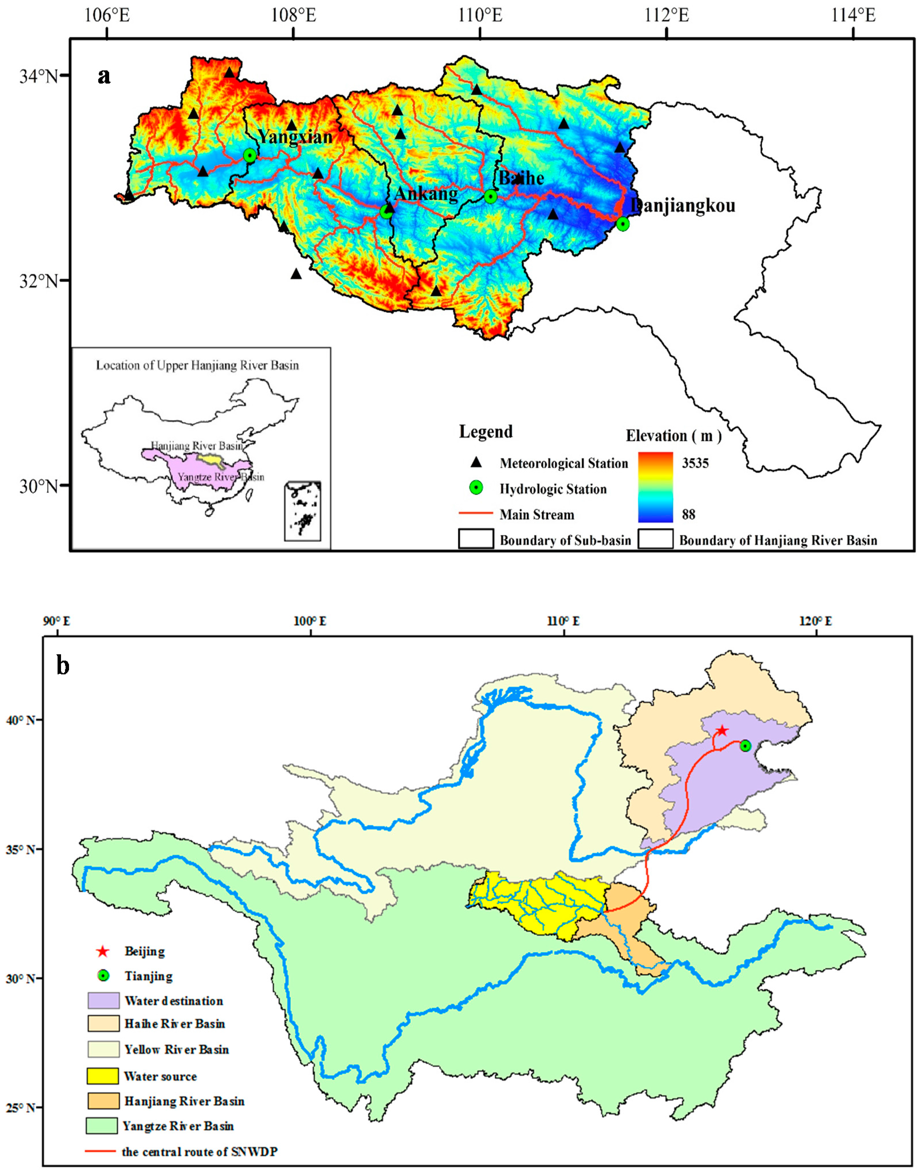
2.1. Study Catchment

The Upper Hanjiang River Basin (UHRB) lies in a subtropical, monsoon-climate region. The altitude of the basin varies from 3535 m in the northwest to 88 m in the southeast, draining to the Danjiangkou reservoir with a drainage area of 95,200 km2 (Figure 1a). The Danjiangkou reservoir is the water source for the central route of China’s South-to-North Water Transfer Project, which plays a critical role in water supply in North China Plain (Figure 1b). This largest water transfer infrastructure is designed to transfer 13 billion m3 yr−1 of water from Danjiangkou reservoir (water source region) to the North China Plain (water destination region) since December 2014 [40]. For better management of Danjiangkou reservoir, it is of critical importance to improve the accuracy of long-term streamflow forecasts in the UHRB. The integral precipitation from July to September (rainy season) accounts for 60% of the total annual precipitation [41]. Four hydrological stations were selected for this study including Yangxian, Ankang, Baihe and Danjiangkou. The four sub-basins area ranges from 14,192 km2 to 95,200 km2. Furthermore, the hydrological stations are also presented in Figure 1a.

2.2. Data

Daily seasonal precipitation and potential evaporation forecasts were sourced from ECMWF System 4. In the analysis, the retrospective forecasts, i.e., hindcasts, in the period from 2001 to 2008 were used. The hindcasts are about 70 km spatial resolution and with a six-month lead time. System 4 issues ensemble forecasts on the first of each month; there are 51 ensemble members in February, May, August and November and 15 ensemble members for other months. In this study, daily ECMWF meteorological forecasts data were aggregated at each representative sub-watershed. For more information on System 4, the reader can refer to Molteni et al. [36].
The daily observed data of precipitation, temperature, wind speed, relative humidity data, etc. for model calibration and evaluation were obtained from the China Meteorological Administration Daily potential evaporation based on the gauged meteorological data was calculated using the Food and Agriculture Organization (FAO) Penman–Monteith Equation [42]. The precipitation and potential evaporation data of each sub-basin are interpolated by the classic Thiessen polygon technique. They are also computed for each representative sub-watershed. Daily streamflow data at Yangxian, Ankang, Baihe and Danjiangkou station were obtained from the Bureau of Hydrology of the Ministry of Water Resources of China. The location of gauging stations is shown in Figure 1a, and the time period of gauged data extends from 2001 to 2008.

3. Method

3.1. Hydrological Model

In this study, Tsinghua Representative Elementary Watershed (THREW) model [43] was used to simulate the hydrological processes. It is a semi-distributed hydrological model which uses the representative elementary watershed approach to conceptualize a watershed [44]. This model has been effectively used in many basins both in the United States and China [45,46,47]. Further, the detailed description and theoretical background of the THREW model can be found in Tian et al. [43,47]. The UHRB is divided into 89 representative elementary watersheds. According to the previous THREW modeling experience and the physical attributes of the UHRB, the initial values and reliable ranges of each parameter were determined in the model calibration [41]. Further, the automatic calibration was carried out with an automatic optimization algorithm, namely, the Non-dominated Sorting Genetic Algorithm II (NSGAII) algorithm [48]. Finally, the parameters were determined automatically. The objective function for the automatic calibration was the Nash–Sutcliffe efficiency coefficient (NSE), which has been widely used in previous studies. Based on the observed gauged data of 1970–2000, THREW model was run at the daily time scale. The model was calibrated for the Baihe station and validated at the Yangxian, Ankang and Danjiangkou stations. The modeling results shown that the annual Nash–Sutcliffe efficiency (NSE) criterion at the four stations (from Yangxian station to Danjiangkou station) in the calibration period were 0.90, 0.88, 0.88 and 0.91, respectively [41].

3.2. Bias Correction Method

An approach introduced by Arlot and Celisse [49], namely, the leave-one-out cross-validation approach is employed in this study. This approach calibrates the bias correction method in each representative elementary watershed over independent periods within the 2001–2008 period. More specifically, for a given target application year, the bias correction method is trained with observations and forecasts from other years. Then, the cross-validation results are applied to the target year for bias correcting.
We applied the quantile mapping method to the original System 4 precipitation forecasts and the linear scaling method to the original System 4 streamflow forecasts. The quantile mapping method matches the statistical distribution of precipitation forecasts to the distribution of observations. In the case of ensemble forecasts, the matching occurs at each ensemble member. The quantile mapping method can be implemented with parametric distribution and non-parametric distribution, however the parametric distribution methods is less influenced by sampling errors and produce more stable mapping functions [21]. In the present study, we adopted the setup of the quantile method as proposed by Lafon et al. [21], namely, Bernoulli-gamma distribution. The Bernoulli distribution fits to the probability of precipitation, whereas the gamma distribution characterizes precipitation amounts larger than zero. For a number of outlying precipitation values, the Bernoulli–gamma distribution could not fit them. In this case, we used a nonparametric empirical cumulative distribution function, which was derived from the precipitation data.
The linear scaling method corrects the monthly ensemble mean values of the forecasts to match the monthly mean values of the observation. The scaling factor was obtained through calculating the ratio between the forecast values and the observed value. Then the monthly scaling factor was applied to each uncorrected daily precipitation forecasts of that month.

3.3. Description of HEPS Method

The hydrological ensemble prediction system (HEPS) method was used as an integrator of the meteorological and hydrological uncertainties [9]. In the HEPS method, the hydrological model state is initialized with observed meteorological forcing through running the model in simulation mode for the year preceding to the time of the forecast. Further, the model with initial basin state was driven by ECMWF System 4 original and bias-correcting ensemble meteorological forecasts. Furthermore, an ensemble of streamflow traces was generated which represents the uncertainty produced by meteorological and hydrological forecasts.
We use the term “QMprep” to describe the bias-corrected original System 4 precipitation forecasts with the quantile mapping method, while the term “LSdis” describes bias-corrected original System 4 streamflow forecasts with linear scaling method. In order to compare the benefits of bias corrected precipitation and bias corrected streamflow, different scenarios of the forecasting experiment are analyzed, including original forecast (without bias-corrected precipitation and bias-corrected streamflow), QMprep forecasts (with bias-corrected precipitation but without bias-corrected streamflow) and LSdis forecasts (without bias-corrected precipitation but with bias-corrected streamflow).

3.4. Forecast Verification

Different scenarios of the forecasts were verified against both deterministic and probabilistic criteria. Four common performance indices were used to assess the forecasting accuracy, including the Nash–Sutcliffe efficiency (NSE), the relative mean error (RME), the coefficient of variation of the root mean squared error (CV) and the correlation coefficient (CC). These metrics have also been widely used in previous studies [50,51,52]. For deterministic analysis, the ensemble forecasts should reduce to single values. In this study, the average of ensemble streamflow forecasts is used to compute deterministic scores in the validation period.
Reliability describes the statistical consistency of forecast probabilities and observed frequencies, which can be assessed with the probability integral transform (PIT) diagram [53]. For a reliable forecast, the observed data should uniformly fall within the prediction distribution and the PIT diagram should accord with the 1:1 diagonal line. According to Laio and Tamea [53], if the scattered points do not lie on the 1:1 line in the PIT diagram, the curve in the PIT diagram generally presents four different shapes, representing four different situations: “over prediction”, “under prediction”, “narrow forecast” and “large forecast”. We also presented the 5% Kolmogorov–Smirnoff confidence interval from the bisector.
The sharpness of the forecasts is evaluated by the interquartile range (IQR), which indicates the spread of an ensemble forecast [54]. To compare IQR among different hydrological stations, the IQR is rescaled by corresponding average discharge, so that IQR becomes dimensionless. The resulting IQR is referred to as the normalized interquartile range (NIQR).
The overall performance of the ensemble forecasts is assessed with the mean ranked probability skill score (mean RPSS). This is defined as the sum of the squared differences of cumulative distribution between the forecast members and observation [55]. The mean RPSS is compared with a reference forecast. Details of both deterministic and probabilistic skill scores are given in Appendix A.

4. Results

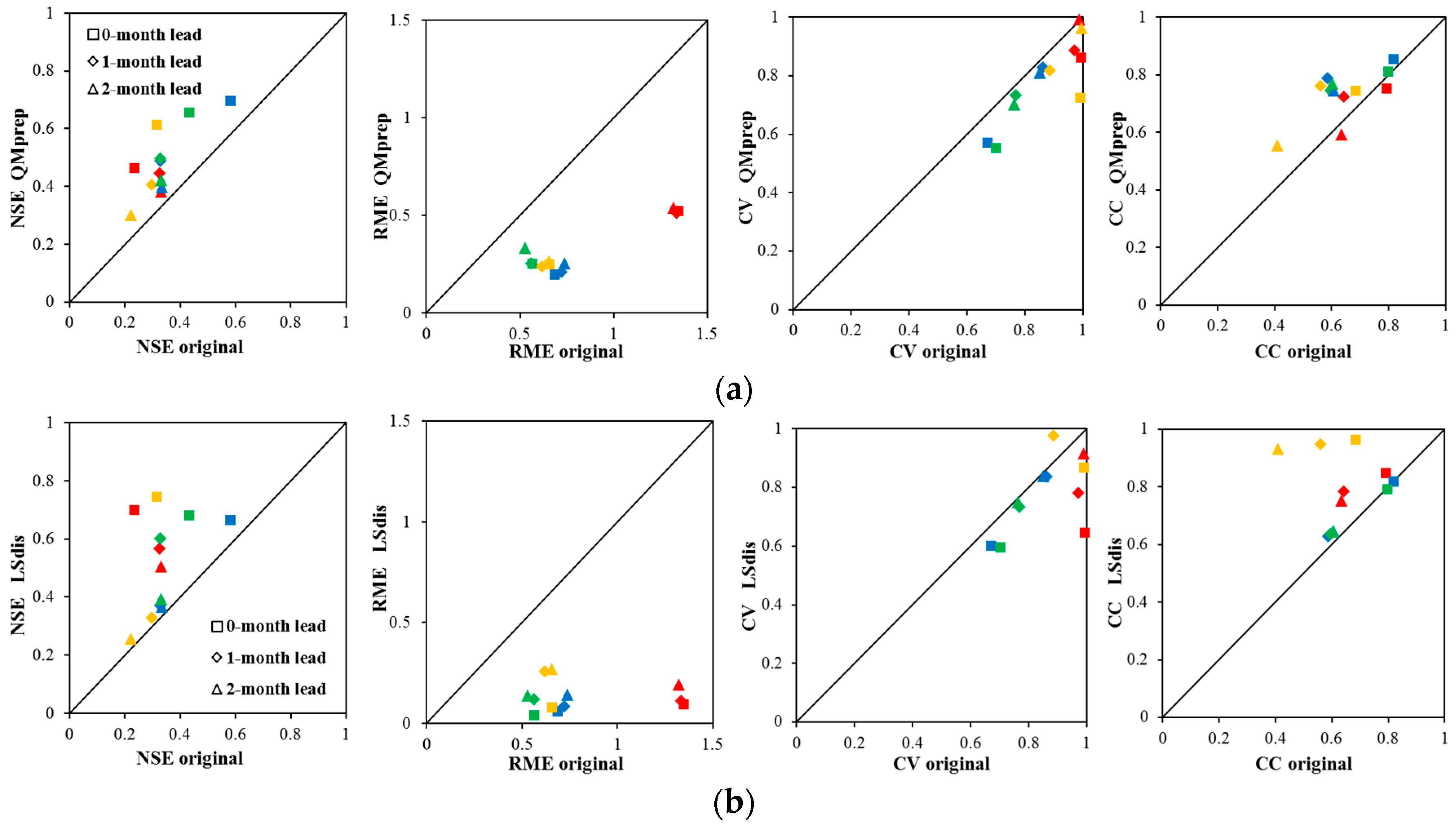
4.1. Forecast Accuracy

Four deterministic scores of bias-corrected forecasts are plotted against the scores for original forecasts in a scatterplot (Figure 2). Deterministic scores for QMprep forecasts are plotted in the upper panel while the deterministic scores for LSdis forecasts are plotted in the lower panel. Each score is computed for lead times of zero-month, one-month and two-month for four stations. It is evident that QMprep forecasts and LSdis forecasts have similar effects in improving deterministic skill scores at different lead times. While the scatterplot of NSE, CV and CC for QMprep forecasts are close to 1:1 line, the skill scores for LSdis forecasts tend to be more accurate than original forecasts. These results demonstrate that LSdis forecasts have a much stronger impact on the accuracy of the forecasts. For instance, in case of the zero-month lead time, the NSEs for the LSdis forecasts were 0.7,0.67,0.74 and 0.68; and for the QMprep forecasts they were 0.46, 0. 67, 0.61 and 0.66 at the four stations, respectively.

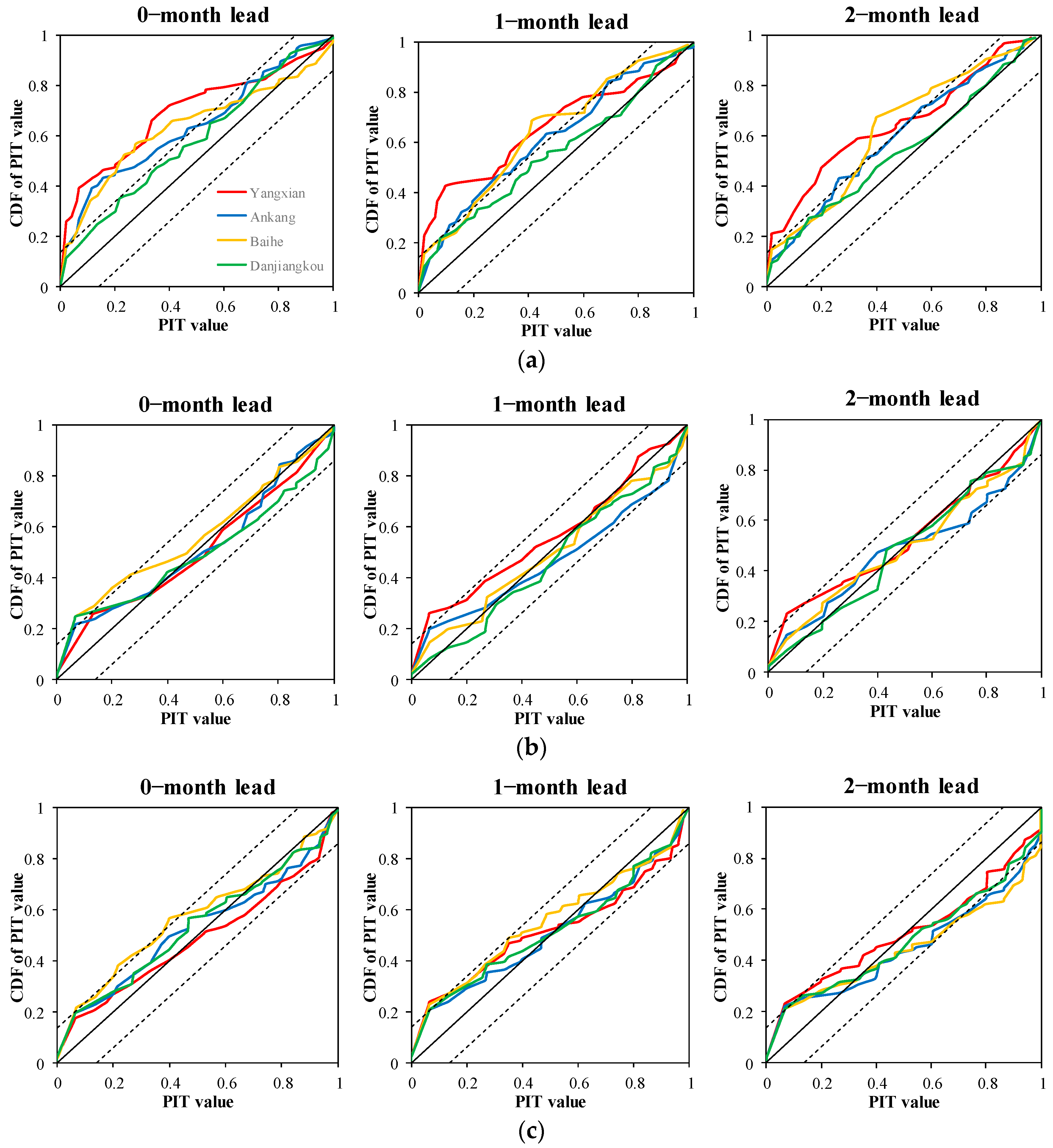
4.2. Forecast Reliability

Figure 3 shows the PIT diagram for each experiment for zero-month, one-month and two-month lead times. The results demonstrated that the streamflow generated from the ECMWF System 4 has an obvious overpredicting bias at different lead times. After bias correcting precipitation by the quantile mapping method, a remarkable improvement is achieved in reliability. This indicates that the quantile mapping method is able to reduce the errors resulting from overestimation of the ECMWF System 4 meteorological forecasts. As the original streamflow forecasts are bias corrected by the linear scaling method, the reliability of forecasts is also improved. It suggests that the bias correcting streamflow generated from the ECMWF System 4 is equally reliable as the bias correcting ECMWF System 4 precipitation. Further, bias correcting streamflow with the linear scaling method from the ECMWF System original streamflow forecast can reduce most of the overestimate bias. Our results confirm the findings of Wetterhall et al. [39], who investigated the bias-correcting ECMWF System 4 seasonal precipitation forecast with the quantile method to improve the skill of forecasts. Zalachori et al. [26] also demonstrated that applying a bias correction method for streamflow forecasts caused significant improvements in forecast reliability.

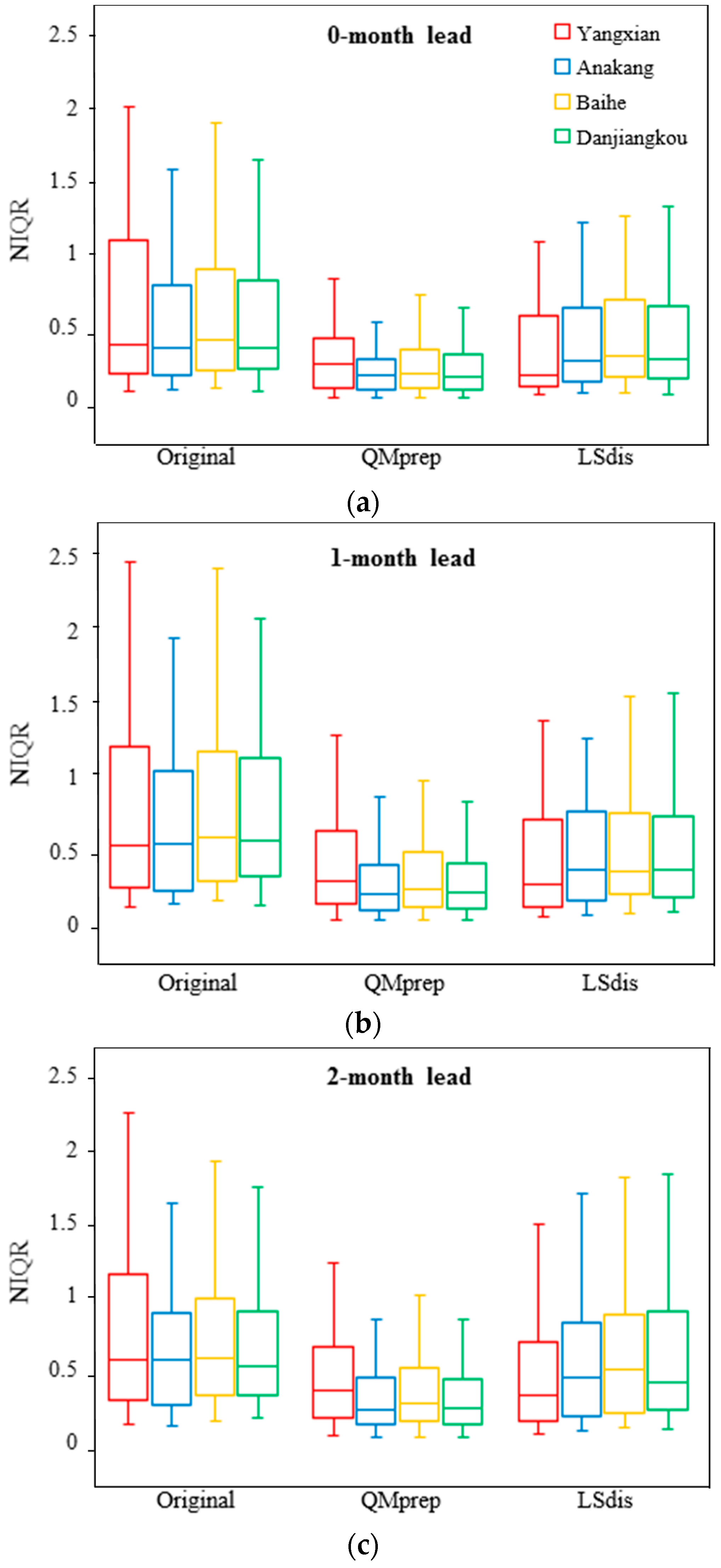
4.3. Forecast Sharpness

Sharpness is an ideal feature of probabilistic forecasts. The narrower the NIQR, the sharper the ensemble forecast, and the less uncertainty is conveyed. Three experiments were used to investigate how meteorological and hydrological uncertainty affects the sharpness of the forecast. Forecast sharpness is described in Figure 4, which presents boxplots of NIQR for different forecast lead times. The boxplots describe the distribution of sharpness for the three experiments. For original forecasts, a striking feature of the NIQR is that the ensemble spread of four sub-basins does not become wider with increasing lead time. For instance, the median values for Danjiangkou station are 0.35, 0.56 and 0.53, with a lead time increasing from zero to two months. It can also be seen that the streamflow obtained directly from System 4 has apparent uncertainties at different lead times. These results indicate that the use of original ECMWF System 4 seasonal climate forecasts in hydrology has problems, which induces stochastic uncertainty in streamflow forecasts. In the QMprep forecasts, the results indicate that bias-corrected precipitation is able to reduce uncertainty from meteorological forcing. The comparison between the QMprep forecast and LSdis forecasts reveals that taking into account hydrological uncertainty leads to less sharpness in the hydrological ensemble prediction system. Furthermore, LSdis forecasts attempt to decrease hydrological uncertainty, thus the ensemble forecast become more spread. This finding is consist with Bourgin et al. [56], who demonstrated that post-processing streamflow forecasts achieved less sharpness.

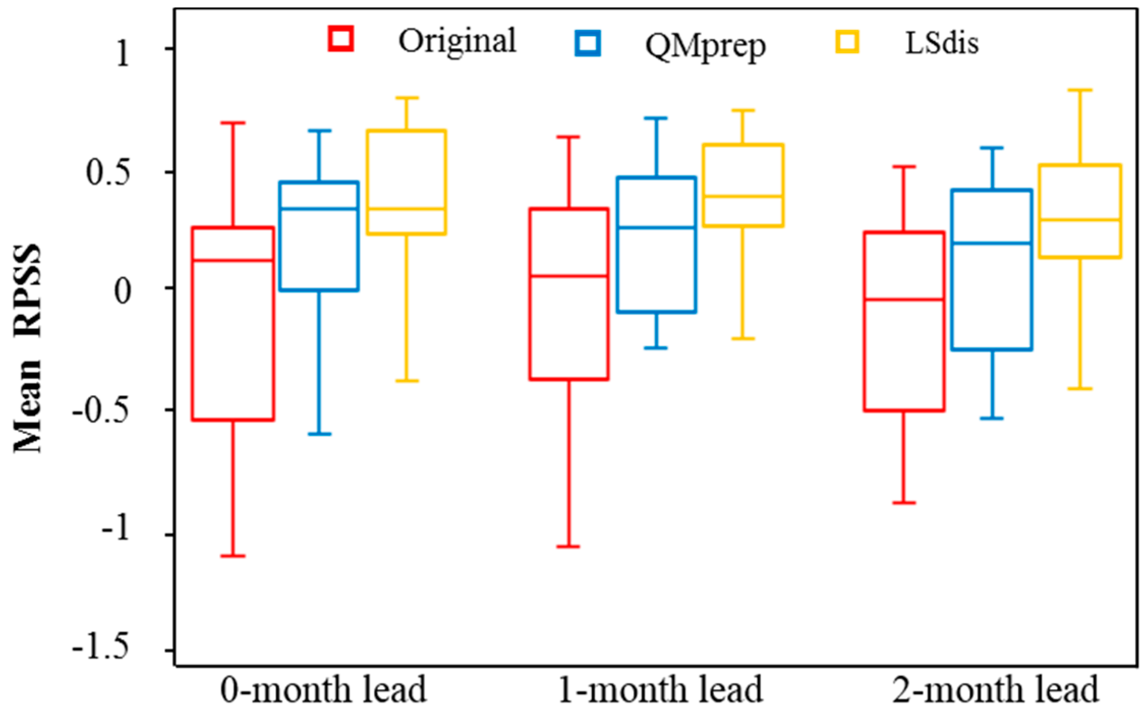
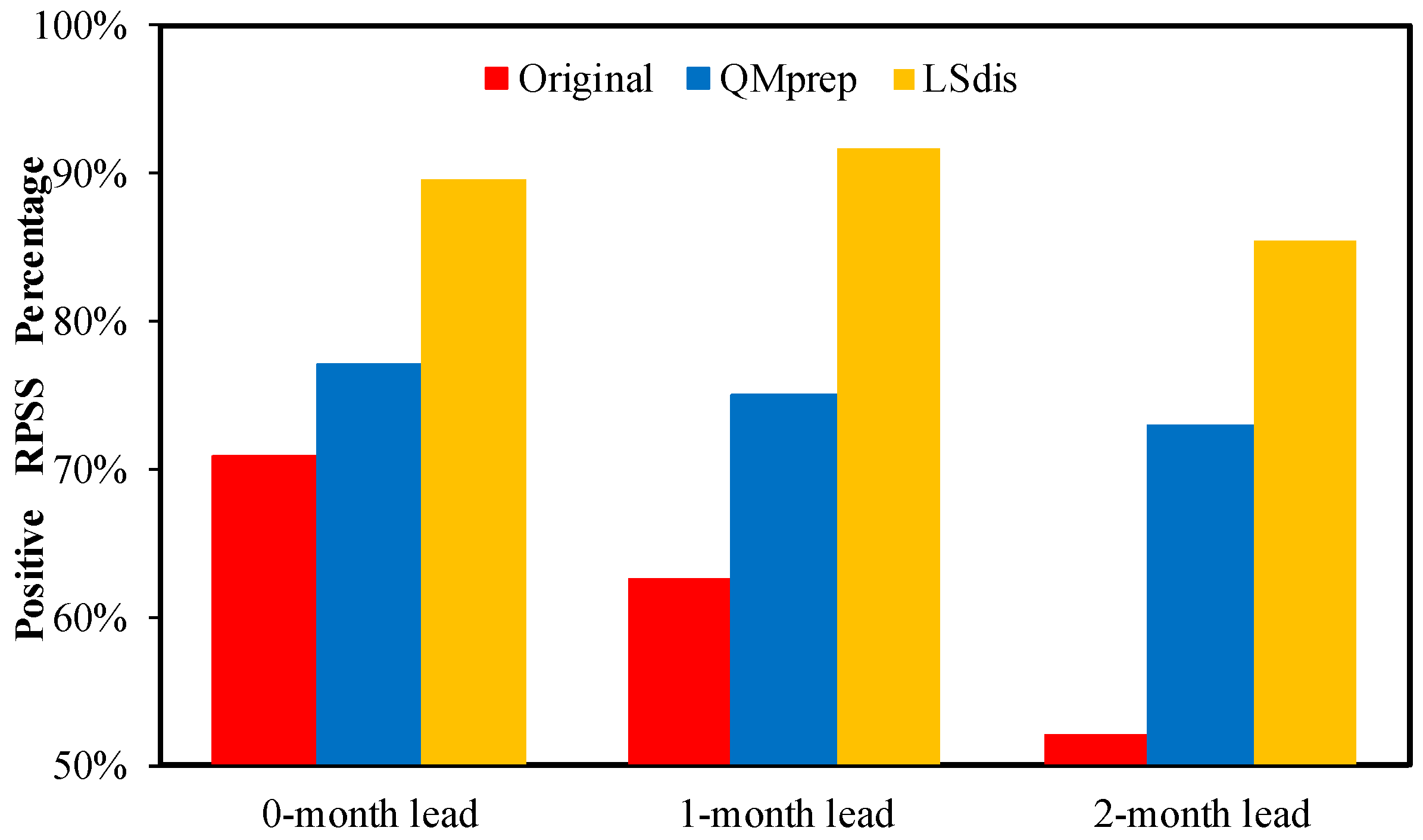
4.4. Forecast Overall Performance

Figure 5 shows the distribution of the mean RPSS over the four stations. Generally, the forecast performance decreases with the extension of lead times. The median values of RPSS were 0.34 (QMprep forecasts) and 0.35 (LSdis forecasts) for the zero-month lead time, and decreased to 0.19 (QMprep forecasts) and 0.29 (LSdis forecasts) for the two-month lead time. The RPSS values of the original forecasts decreased slightly with the lead times, which ranged from 0.12 for the zero-month lead time to −0.04 for the two-month lead times. Furthermore, the RPSS value of the original forecasts were much lower than the values obtained with the QMprep and LSdis forecasts.
The percentage of positive RPSS is shown in Figure 6, which presents the frequency of forecasts that are more competent against the reference forecast. The ability of all forecasts decreases as the forecast lead time increases. Without bias correction, the original streamflow forecasts have a negligible advantage against reference forecast beyond the one-month lead time. QMprep forecasts present as more skillful than reference forecasts at the two-month lead time. Compared with original forecasts, LSdis forecasts show moderate improvement at the zero-month lead time and remarkable improvement at the two-month lead time. Our results are consist with Yuan and Wood [17], as they showed that bias-corrected GCM streamflow was more skillful than downscaling precipitation for hydrologic modeling in terms of RPSS. Our study also shows that bias-corrected streamflow has a more positive effect on ensemble forecasts, as verified by the RPSS.

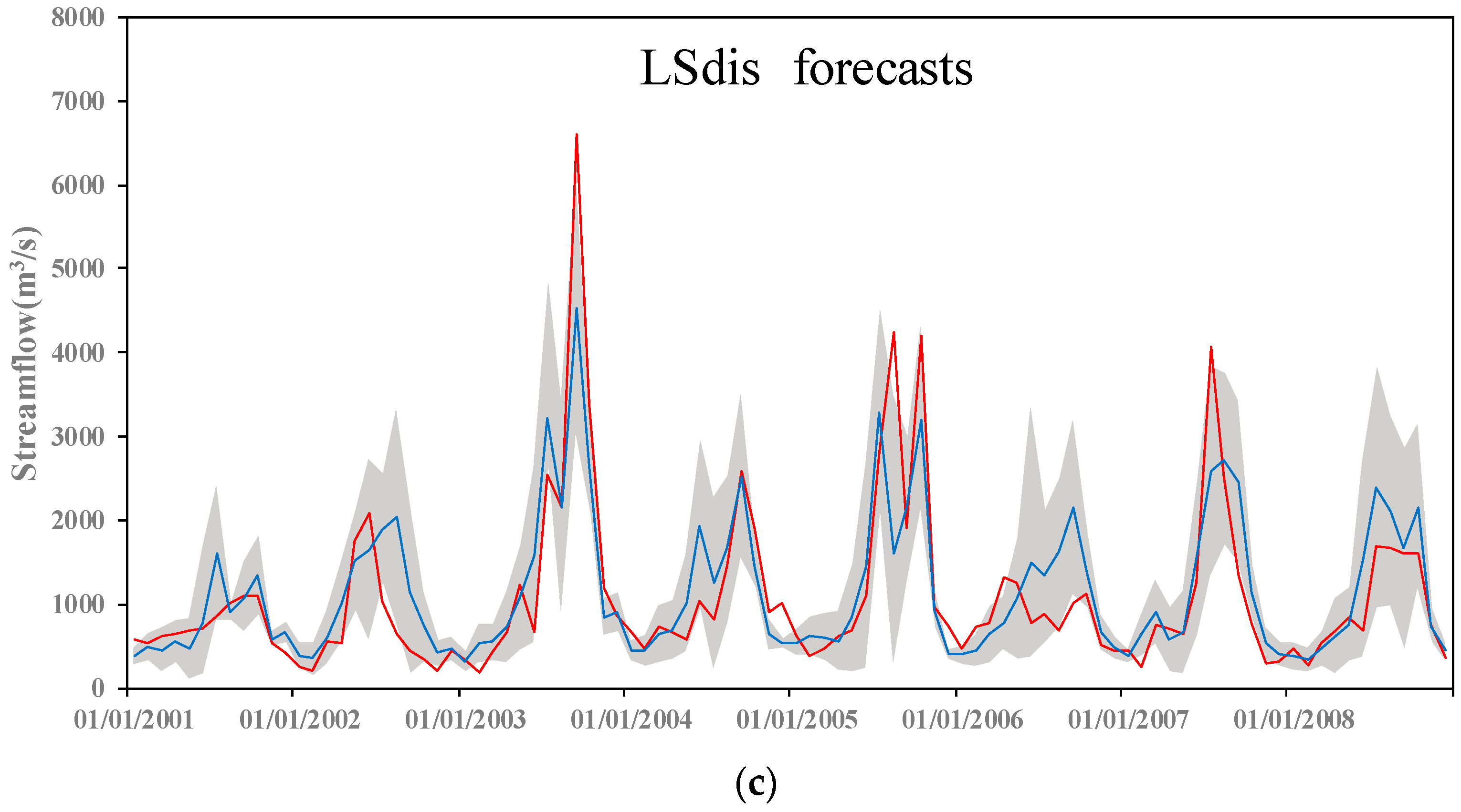
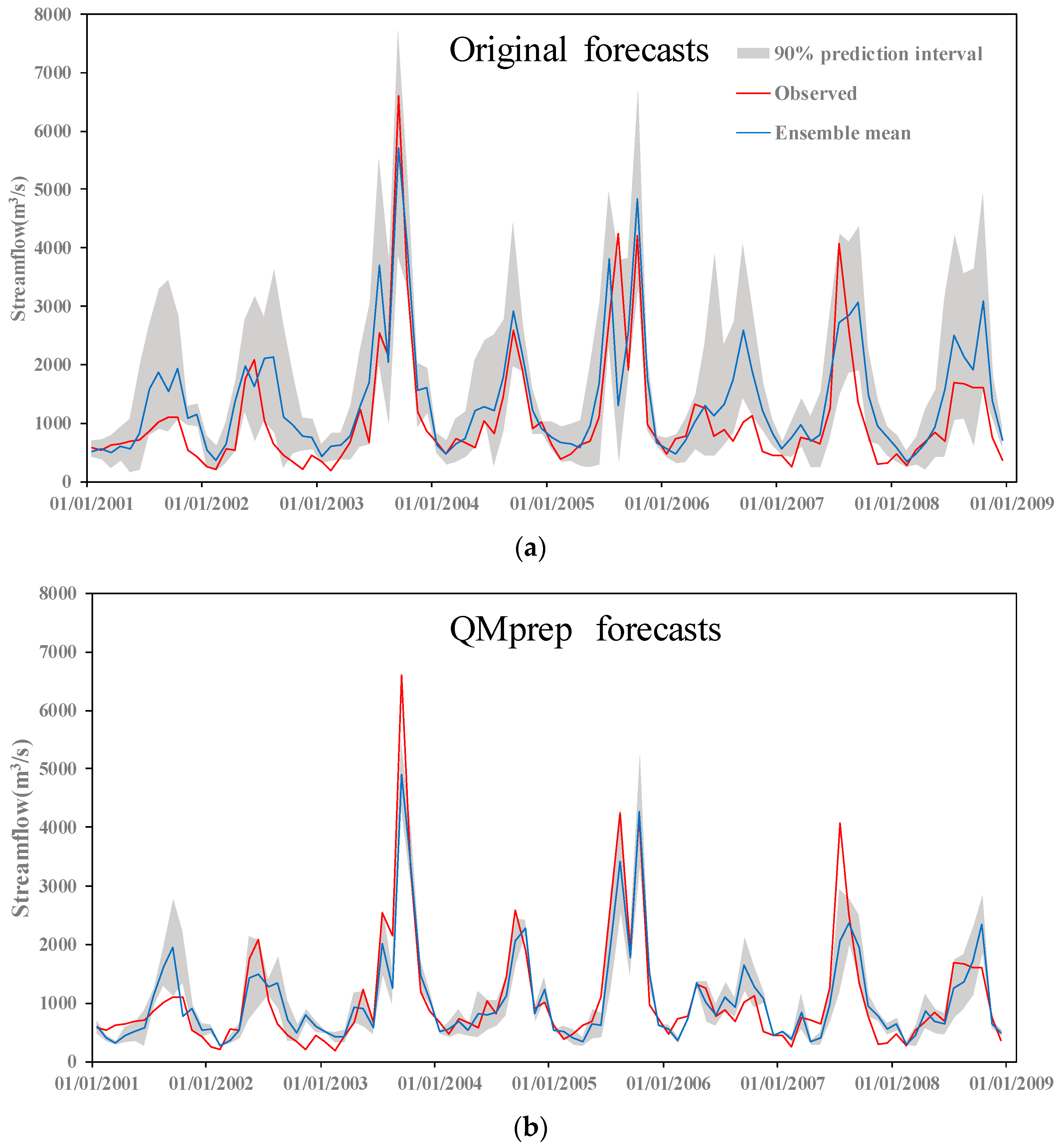
4.5. Forecast Hydrographs Illustration

Figure 7 presents the hydrographs of the forecasts obtained from the original, QMprep and LSdis forecasts for the time period of January 2001 to December 2008 in Danjiangkou station. Here we only show the results for the zero-month lead time, because the performances of different lead times are similar. Ensemble forecasts are represented by the ensemble mean value (blue line) and 90% credible intervals (gray zone). Observed streamflow is represented by the red line. The hydrograph of the original forecasts is the least accurate and the dose does not capture the low flows. However, the streamflow forecasts obtained from the QMprep forecasts shows remarkable improvements in the sharpness, especially during low flow periods. The hydrograph of LSdis forecasts also shows improvement when comparing with the original forecasts. In general, the coverage of 90% credible intervals of QMprep forecasts more accurately capture the observed streamflow than LSdis forecasts, which indicates that QMprep forecasts have a more positive effect on forecast reliability.

5. Discussion

The present study considered the quantile mapping method to bias correct precipitation forecasts and the linear scaling method to bias correct streamflow forecasts. Zhao et al. [35] demonstrated that the quantile mapping method could effectively remove bias when the bias was the main deficiency of the raw forecasts, e.g., ECMWF System 4 precipitation forecasts, Predictive Ocean–Atmosphere Model for Australia (POAMA) model precipitation forecasts. They also found that quantile mapping method could not correct the overconfidence of the raw ensemble spread. Several other bias correction approaches were also used in the previous literature, including model output statistics [57], event bias correction [58], Bayesian model average [14] and Bayesian joint probability [33]. These could be applied as preferable options to bias correct precipitation and streamflow forecasts for ensemble streamflow forecasts. Besides, the benefit of bias correcting precipitation forecasts and bias correcting original streamflow forecasts is influenced by multiple sources of uncertainty in a hydrological ensemble prediction system, including meteorological forcing, hydrological models, model parameter uncertainty and initial hydrological conditions. Our study only focused on bias correcting where the bias comes from meteorological forcing and the hydrological model. Additional analysis could be necessary to better investigate which is the primary factor affecting the ensemble streamflow forecast skill. Further, the hydrological model carried out in this study is a semi-distributed hydrological model, which was set up on 89 sub-watersheds. The Thiessen polygon method, which was used this study to obtain the input meteorological data, has been frequently applied to such sub-watershed based modeling practices with satisfactory results. For example, in our study area (Upper Hanjiang River Basin), Sun et al. [41] and Yang et al. [59] demonstrated that the rainfall runoff process was simulated rather well with the same interpolation method and hydrological model. The values of daily NSE in both the calibration and validation periods were above 0.80. The value of the monthly NSE was as high as 0.99. Lastly, we only chosen the Upper Hanjiang River Basin as a case study, which is not influenced by snowmelt flow; while in snow-dominant basins in China, bias-correcting temperature forecasts also can be considered.

6. Conclusions

This study investigated the benefits of bias-correcting ECMWF System 4 precipitation forecasts and bias-correcting ECMWF System 4 original streamflow for improving the overall accuracy of the hydrological ensemble prediction system in Upper Hanjiang River Basin. The effect of bias-corrected precipitation and bias-corrected streamflow were evaluated with three experiments, namely, original forecasts (without bias-corrected precipitation and streamflow), QMprep forecasts (bias-corrected precipitation with the quantile mapping method), and LSdis forecasts (bias-corrected streamflow with the linear scaling method). The performance of the ensemble streamflow forecast was assessed in terms of the forecast accuracy, reliability, sharpness and overall performance.
Compared to original forecasts, bias-correcting precipitation or bias-correcting streamflow is necessary to correct overestimation/underestimation of the ensemble, which preforms considerably better in terms of both deterministic and probabilistic skill scores. However, the benefits of the bias-correcting GCM forcing and bias-correcting hydrologic output present variables in ensemble streamflow forecasts. Bias-correcting precipitation has a strong impact on improving forecast reliability and sharpness, while bias-correcting streamflow has a more positive effect on forecast accuracy and the overall quality of the ensemble forecast. Further, the use of both bias-correcting GCM forecasts and bias-correcting hydrologic output is highly recommended, which may achieve ideal forecast performance.

Acknowledgments

This research was supported by Ministry of Science and Technology of P.R. China (2016YFC0402701), the National Science Foundation of China (NSFC 91647205), Ministry of Science and Technology of P.R. China (2016YFA0601603), the foundation of State Key Laboratory of Hydroscience and Engineering of Tsinghua University (2016-KY-03). The authors would like to thank the Information Center of Ministry of Water Resources and China Meteorological Administration for providing the hydrology and meteorological data.

Author Contributions

Y.L., F.T. and X.L. conceived and designed the study; Y.L., Y.J. and H.D. performed the modeling experiments; Y.L, Y.J. and H.L. analyzed the results; Y.L. wrote the paper and all of the authors contributed to the paper writing.

Conflicts of Interest

The authors declare no conflict of interest.

Appendix A

Appendix A.1. Deterministic Verification Metrics

Appendix A.1.1. Nash–Sutcliffe Efficiency

N S E = 1 t = 1 N [ q o b s ( t ) q f c ( t ) ] 2 t = 1 N [ q o b s ( t ) q ¯ o b s ( t ) ] 2
where q o b s ( t ) is the observed value, q f c ( t ) is the corresponding ensemble forecasts value and q ¯ o b s ( t ) is the average of observed values. The NSE values range from −∞ to 1. For a perfect forecast, NSE equals to 1.

Appendix A.1.2. Relative Mean Error

The relative mean error (RME) measures the difference between a series of forecasts and corresponding observations.
R M E = 1 N t = 1 N [ q f c ( t ) q o b s ( t ) ] t = 1 N q o b s ( t )
where ( q f c ( t ) , q o b s ( t ) ) is the tth of N pairs of forecasts and observation. A positive RME indicates overestimation, whereas negative RME indicates underestimation. For an ideal forecasts, RME equals to 0.

Appendix A.1.3. Coefficient Variation of Root Mean Squared Error

The root mean squared error (RMSE) represents the standard deviation of the differences between forecast values and observed values. The coefficient variation of root mean squared error (CV) is rescaled by the average discharge that facilitates the comparison of RMSE values among different hydrological stations.
C V = t = 1 N [ q o b s ( t ) q f c ( t ) ] 2 N q ¯ o b s
where ( q f c ( t ) , q o b s ( t ) ) is the tth of N pairs of observed value and forecast value, the q ¯ o b s ( t ) is the average of observed values. A lower CV score corresponds to a better forecast.

Appendix A.1.4. Correlation Coefficient

The correlation coefficient (CC) measures the linear dependency between forecasts and observations.
C C = t = 1 N ( q o b s ( t ) q ¯ o b s ) ( q f c ( t ) q ¯ f c ) t = 1 N ( q o b s ( t ) q ¯ o b s ) 2 i = 1 N ( q f c ( t ) q ¯ f c ) 2
q o b s , q f c , q ¯ o b s and q ¯ f c represents the observed value, the forecast value, the average of observed values and the average of forecast values respectively. The CC values range from 0 to 1, the latter corresponding to perfect forecasts.

Appendix A.2. Probabilistic Verification Metrics

Appendix A.2.1. Probability Integral Transform (PIT) Diagram

The probability integral transform (PIT) diagram represents the distribution of PIT values, which is defined by the observed values falling within the prediction distribution. For a reliable forecast, the PIT diagram should accord with the 1:1 diagonal. The PIT values is calculated as follow:
P I T t = F t ( q o b s , t )
where F t is the cumulative distribution function of the forecast, q o b s , t is the corresponding observed data, t = 1, 2, …, N , and N is the number of observations.

Appendix A.2.2. Normalized Interquartile Range

The interquartile range is computed as the range between 75th and 25th percentiles of the spread of forecast distribution.
N I Q R = t = 1 N q f c 75 ( t ) q f c 25 ( t ) q o b s ¯
where the q f c 75 ( t ) and q f c 25 ( t ) is the tth of the 75th and 25th percentile of the forecast distribution respectively.

Appendix A.2.3. Mean Rank Probability Skill Score

The rank probability score (RPS) measures how well the probability forecast predicts the corresponding observations (Wilks, 2011).
R P S = m = 1 J [ ( j = 1 m Y f c , j j = 1 m O o b s , j ) 2 ]
where Y f c refers to the relative occurrence frequency of ensemble members in the corresponding category, O o b s represents the observation probability in the category, and J is the number of categories. In this study, we divided ensemble streamflow into three categories: above normal category, near normal category and below normal category.
The R P S ¯ is the average RPS value of forecast data. The mean rank skill score (RPSS) is based on the RPS, which is compared with a reference forecast (Wilks, 2011).
R P S S = 1 R P S f ¯ R P S ¯ r e f
where R P S f ¯ is the average RPS for ensemble forecast and R P S ¯ r e f is the average RPS for reference forecast.

References

  1. Alemu, E.T.; Palmer, R.N.; Polebitski, A.; Meaker, B. Decision support system for optimizing reservoir operations using ensemble streamflow predictions. J. Water Res. Plan. Manag. 2011, 137, 72–82. [Google Scholar] [CrossRef]
  2. Chiew, F.H.S.; Zhou, S.L.; McMahon, T.A. Use of seasonal streamflow forecasts in water resources management. J. Hydrol. 2003, 270, 135–144. [Google Scholar] [CrossRef]
  3. Maurer, E.P.; Lettenmaier, D.P. Potential effects of long-lead hydrologic predictability on Missouri River main-stem reservoirs. J. Clim. 2004, 17, 174–186. [Google Scholar] [CrossRef]
  4. Khan, M.Y.A.; Hasan, F.; Panwar, S.; Chakrapani, G.J. Neural network model for discharge and water-level prediction for Ramganga River catchment of Ganga Basin, India. Hydrol. Sci. J. 2016, 61, 2084–2095. [Google Scholar] [CrossRef]
  5. Cloke, H.L.; Pappenberger, F. Ensemble flood forecasting: A review. J. Hydrol. 2009, 375, 613–626. [Google Scholar] [CrossRef]
  6. Zhao, T.; Zhao, J. Joint and respective effects of long- and short-term forecast uncertainties on reservoir operations. J. Hydrol. 2014, 517, 83–94. [Google Scholar] [CrossRef]
  7. Chen, Y.D.; Zhang, Q.; Xiao, M.; Singh, V.P.; Zhang, S. Probabilistic forecasting of seasonal droughts in the Pearl River basin, China. Stoch. Environ. Res. Risk Assess. 2015, 30, 2031–2040. [Google Scholar] [CrossRef]
  8. Easey, J.; Prudhomme, C.; Hannah, D.M. Seasonal forecasting of river flows: A review of the state-of-the-art. IAHS Publ. 2006, 308, 158–162. [Google Scholar]
  9. Schaake, J.C.; Hamill, T.M.; Buizza, R.; Clark, M. HEPEX: The Hydrological ensemble prediction experiment. Bull. Am. Meteorol. Soc. 2007, 88, 1541–1547. [Google Scholar] [CrossRef]
  10. Hamill, T.M.; Hagedorn, R.; Whitaker, J.S. Probabilistic forecast calibration using ECMWF and GFS ensemble reforecasts. Part II: Precipitation. Mon. Weather Rev. 2008, 136, 2620–2632. [Google Scholar] [CrossRef]
  11. Roulin, E.; Vannitsem, S. Postprocessing of ensemble precipitation predictions with extended logistic regression based on hindcasts. Mon. Weather Rev. 2012, 140, 874–888. [Google Scholar] [CrossRef]
  12. Bremnes, J.B. Probabilistic forecasts of precipitation in terms of quantiles using NWP model output. Mon. Weather Rev. 2004, 132, 338–347. [Google Scholar] [CrossRef]
  13. Friederichs, P.; Hense, A. A probabilistic forecast approach for daily precipitation totals. Weather Forecast. 2008, 23, 659–673. [Google Scholar] [CrossRef]
  14. Raftery, A.E.; Gneiting, T.; Balabdaoui, F.; Polakowski, M. Using Bayesian model averaging to calibrate forecast ensembles. Mon. Weather Rev. 2005, 133, 1155–1174. [Google Scholar] [CrossRef]
  15. Schmeits, M.J.; Kok, K.J. A Comparison between raw ensemble output, (modified) Bayesian model averaging, and extended logistic regression using ECMWF ensemble precipitation reforecasts. Mon. Weather Rev. 2010, 138, 4199–4211. [Google Scholar] [CrossRef]
  16. Hamill, T.M.; Whitaker, J.S.; Wei, X. Ensemble reforecasting: Improving medium-range forecast skill using retrospective forecasts. Mon. Weather Rev. 2004, 132, 1434–1447. [Google Scholar] [CrossRef]
  17. Yuan, X.; Wood, E.F. Downscaling precipitation or bias-correcting streamflow? Some implications for coupled general circulation model (CGCM)-based ensemble seasonal hydrologic forecast. Water Resour. Res. 2012, 48, 12519. [Google Scholar] [CrossRef]
  18. Yuan, X.; Wood, E.F.; Ma, Z. A review on climate-model-based seasonal hydrologic forecasting: Physical understanding and system development. Wiley Interdiscip. Rev. Water 2015, 2, 523–536. [Google Scholar] [CrossRef]
  19. Wood, A.W.; Lettenmaier, D.P. A Test Bed for New Seasonal Hydrologic Forecasting Approaches in the Western United States. Bull. Am. Meteorol. Soc. 2006, 87, 1699–1712. [Google Scholar] [CrossRef]
  20. Piani, C.; Haerter, J.O.; Coppola, E. Statistical bias correction for daily precipitation in regional climate models over Europe. Theor. Appl. Climatol. 2009, 99, 187–192. [Google Scholar] [CrossRef]
  21. Lafon, T.; Dadson, S.; Buys, G.; Prudhomme, C. Bias correction of daily precipitation simulated by a regional climate model: A comparison of methods. Int. J. Climatol. 2013, 33, 1367–1381. [Google Scholar] [CrossRef] [Green Version]
  22. Hashino, T.; Bradley, A.A.; Schwartz, S.S. Evaluation of bias-correction methods for ensemble streamflow volume forecasts. Hydrol. Earth Syst. Sci. 2007, 11, 939–950. [Google Scholar] [CrossRef]
  23. Kang, T.-H.; Kim, Y.-O.; Hong, I.-P. Comparison of pre- and post-processors for ensemble streamflow prediction. Atmos. Sci. Lett. 2010, 11, 153–159. [Google Scholar] [CrossRef]
  24. Wood, A.W.; Schaake, J.C. Correcting errors in streamflow forecast ensemble mean and spread. J. Hydrometeorol. 2008, 9, 132–148. [Google Scholar] [CrossRef]
  25. Roy, T.; Serrat-Capdevila, A.; Gupta, H.; Valdes, J. A platform for probabilistic multimodel and multiproduct streamflow forecasting. Water Resour. Res. 2017, 53, 376–399. [Google Scholar] [CrossRef]
  26. Zalachori, I.; Ramos, M.H.; Garçon, R.; Mathevet, T.; Gailhard, J. Statistical processing of forecasts for hydrological ensemble prediction: A comparative study of different bias correction strategies. Adv. Sci. Res. 2012, 8, 135–141. [Google Scholar] [CrossRef]
  27. Trambauer, P.; Werner, M.; Winsemius, H.C.; Maskey, S.; Dutra, E.; Uhlenbrook, S. Hydrological drought forecasting and skill assessment for the Limpopo River basin, southern Africa. Hydrol. Earth Syst. Sci. 2015, 19, 1695–1711. [Google Scholar] [CrossRef]
  28. Wood, A.W. Long-range experimental hydrologic forecasting for the eastern United States. J. Geophys. Res. 2002, 107. [Google Scholar] [CrossRef]
  29. Shi, X.; Wood, A.W.; Lettenmaier, D.P. How Essential is hydrologic model calibration to seasonal streamflow forecasting? J. Hydrometeorol. 2008, 9, 1350–1363. [Google Scholar] [CrossRef]
  30. Crochemore, L.; Ramos, M.-H.; Pappenberger, F. Bias correcting precipitation forecasts to improve the skill of seasonal streamflow forecasts. Hydrol. Earth Syst. Sci. 2016, 20, 3601–3618. [Google Scholar] [CrossRef]
  31. Clark, M.; Gangopadhyay, S.; Hay, L.; Rajagopalan, B.; Wilby, R. The Schaake shuffle: A method for reconstructing space-time variability in forecasted precipitation and temperature fields. J. Hydrometeorol. 2004, 5, 243–262. [Google Scholar] [CrossRef]
  32. Luo, L.; Wood, E.F.; Pan, M. Bayesian merging of multiple climate model forecasts for seasonal hydrological predictions. J. Geophys. Res. 2007, 112. [Google Scholar] [CrossRef]
  33. Wang, Q.J.; Robertson, D.E.; Chiew, F.H.S. A Bayesian joint probability modeling approach for seasonal forecasting of streamflows at multiple sites. Water Resour. Res. 2009, 45, 641–648. [Google Scholar] [CrossRef]
  34. Schepen, A.; Wang, Q.J. Ensemble forecasts of monthly catchment rainfall out to long lead times by post-processing coupled general circulation model output. J. Hydrol. 2014, 519, 2920–2931. [Google Scholar] [CrossRef]
  35. Zhao, T.; Bennett, J.C.; Wang, Q.J.; Schepen, A.; Wood, A.W.; Robertson, D.E.; Ramos, M.-H. How Suitable Is Quantile Mapping for Postprocessing GCM Precipitation Forecasts? J. Clim. 2017, 30, 3185–3196. [Google Scholar] [CrossRef]
  36. Molteni, F.; Stockdale, T.; Balmaseda, M.; Balsamo, G.; Buizza, R.; Ferranti, L.; Magnusson, L.; Mogensen, K.; Palmer, T. The New ECMWF Seasonal Forecast System (System 4); European Centre for Medium Range Weather Forecasts (ECMWF): Reading, UK, 2011. [Google Scholar]
  37. Peng, Z.; Wang, Q.J.; Bennett, J.C.; Schepen, A.; Pappenberger, F.; Pokhrel, P.; Wang, Z. Statistical calibration and bridging of ECMWF System4 outputs for forecasting seasonal precipitation over China. J. Geophys. Res. Atmos. 2014, 119, 7116–7135. [Google Scholar] [CrossRef]
  38. Kim, H.-M.; Webster, P.J.; Curry, J.A. Seasonal prediction skill of ECMWF System 4 and NCEP CFSv2 retrospective forecast for the Northern Hemisphere winter. Clim. Dyn. 2012, 39, 2957–2973. [Google Scholar] [CrossRef]
  39. Wetterhall, F.; Winsemius, H.C.; Dutra, E.; Werner, M.; Pappenberger, E. Seasonal predictions of agro-meteorological drought indicators for the Limpopo basin. Hydrol. Earth Syst. Sci. 2015, 19, 2577–2586. [Google Scholar] [CrossRef]
  40. Liu, X.; Luo, Y.; Yang, T.; Liang, K.; Zhang, M.; Liu, C. Investigation of the probability of concurrent drought events between the water source and destination regions of China’s water diversion project. Geophys. Res. Lett. 2015, 42, 8424–8431. [Google Scholar] [CrossRef]
  41. Sun, Y.; Tian, F.; Yang, L.; Hu, H. Exploring the spatial variability of contributions from climate variation and change in catchment properties to streamflow decrease in a mesoscale basin by three different methods. J. Hydrol. 2014, 508, 170–180. [Google Scholar] [CrossRef]
  42. Allen, R.G.; Pereira, L.S.; Raes, D.; Smith, M. Crop Evapotranspiration-Guidelines for Computing Crop Water Requirements-FAO Irrigation and Drainage Paper 56; Food and Agriculture Organization (FAO): Rome, Italy, 1998; Volume 300, p. D05109. [Google Scholar]
  43. Tian, F.; Hu, H.; Lei, Z.; Sivapalan, M. Extension of the Representative Elementary Watershed approach for cold regions via explicit treatment of energy related processes. Hydrol. Earth Syst. Sci. 2006, 10, 619–644. [Google Scholar] [CrossRef]
  44. Reggiani, P.; Sivapalan, M.; Hassanizadeh, S.M. A unifying framework for watershed thermodynamics: Balance equations for mass, momentum, energy and entropy, and the second law of thermodynamics. Adv. Water Resour. 1998, 22, 367–398. [Google Scholar] [CrossRef]
  45. He, Z.H.; Tian, F.Q.; Gupta, H.V.; Hu, H.C.; Hu, H.P. Diagnostic calibration of a hydrological model in a mountain area by hydrograph partitioning. Hydrol. Earth Syst. Sci. 2015, 19, 1807–1826. [Google Scholar] [CrossRef]
  46. Li, H.; Sivapalan, M.; Tian, F. Comparative diagnostic analysis of runoff generation processes in Oklahoma DMIP2 basins: The Blue River and the Illinois River. J. Hydrol. 2012, 418–419, 90–109. [Google Scholar] [CrossRef]
  47. Tian, F.; Li, H.; Sivapalan, M. Model diagnostic analysis of seasonal switching of runoff generation mechanisms in the Blue River basin, Oklahoma. J. Hydrol. 2012, 418–419, 136–149. [Google Scholar] [CrossRef]
  48. Reed, P.; Minsker, B.S.; Goldberg, D.E. Simplifying multiobjective optimization: An automated design methodology for the nondominated sorted genetic algorithm-II. Water Resour. Res. 2003, 39, 257–271. [Google Scholar] [CrossRef]
  49. Arlot, S.; Celisse, A. A survey of cross-validation procedures for model selection. Stat. Surv. 2010, 4, 40–79. [Google Scholar] [CrossRef]
  50. Alfieri, L.; Pappenberger, F.; Wetterhall, F.; Haiden, T.; Richardson, D.; Salamon, P. Evaluation of ensemble streamflow predictions in Europe. J. Hydrol. 2014, 517, 913–922. [Google Scholar] [CrossRef]
  51. Renner, M.; Werner, M.G.F.; Rademacher, S.; Sprokkereef, E. Verification of ensemble flow forecasts for the River Rhine. J. Hydrol. 2009, 376, 463–475. [Google Scholar] [CrossRef]
  52. Verkade, J.S.; Brown, J.D.; Reggiani, P.; Weerts, A.H. Post-processing ECMWF precipitation and temperature ensemble reforecasts for operational hydrologic forecasting at various spatial scales. J. Hydrol. 2013, 501, 73–91. [Google Scholar] [CrossRef]
  53. Laio, F.; Tamea, S. Verification tools for probabilistic forecasts of continuous hydrological variables. Hydrol. Earth Syst. Sci. 2007, 11, 1267–1277. [Google Scholar] [CrossRef]
  54. Gneiting, T.; Balabdaoui, F.; Raftery, A.E. Probabilistic forecasts, calibration and sharpness. J. R. Stat. Soc. B 2007, 69, 243–268. [Google Scholar] [CrossRef]
  55. Wilks, D.S. Statistical Methods in the Atmospheric Sciences; Academic Press: Cambridge, MA, USA, 2011; Volume 100. [Google Scholar]
  56. Bourgin, F.; Ramos, M.H.; Thirel, G.; Andréassian, V. Investigating the interactions between data assimilation and post-processing in hydrological ensemble forecasting. J. Hydrol. 2014, 519, 2775–2784. [Google Scholar] [CrossRef]
  57. Gneiting, T.; Raftery, A.E.; Westveld, A.H.; Goldman, T. Calibrated probabilistic forecasting using ensemble model output statistics and minimum CRPS estimation. Mon. Weather Rev. 2005, 133, 1098–1118. [Google Scholar] [CrossRef]
  58. Smith, J.A.; Day, G.N.; Kane, M.D. Nonparametric framework for long-range streamflow forecasting. J. Water Res. Plan. Manag. 1992, 118, 82–92. [Google Scholar] [CrossRef]
  59. Yang, L.; Tian, F.; Sun, Y.; Yuan, X.; Hu, H. Attribution of hydrologic forecast uncertainty within scalable forecast windows. Hydrol. Earth Syst. Sci. 2014, 18, 775–786. [Google Scholar] [CrossRef] [Green Version]
Figure 1. (a) Overview of the Upper Hanjiang River Basin (UHRB); (b) overview of the central of China’s South to North Water Diversion Project (SNWDP).
Water 10 00177 g001
Figure 2. Scatterplots of four deterministic scores, the Nash–Sutcliffe efficiency (NSE), the relative mean error (RME), the coefficient of variation of the root mean squared error (CV) and the correlation coefficient (CC) for different lead times. The scatterplots plot bias-corrected original System 4 precipitation forecasts with quantile mapping method (QMprep) forecasts skill scores (a) and bias-corrected original System 4 streamflow forecasts with linear scaling method (LSdis) forecasts skill scores (b) against original forecasts skill scores, respectively. Each color represents the skill scores in a station for forecast horizons within the lead times.
Water 10 00177 g002
Figure 3. Probability integral transform (PIT) diagram of streamflow forecasts obtained from original forecast (a), QMprep forecasts (b) and LSdis forecasts (c) for different lead times. Each line represents the PIT diagram at a station. Dotted dark lines represent the 5% Kolmogorov–Smirnoff confidence bands.
Water 10 00177 g003
Figure 4. Distribution of normalized interquartile range (NIQR) for ensemble streamflow forecasts in the four stations with (a) zero-month lead times; (b) one-month lead times and (c) two-month lead times. Results for three experiments of forecasts are presented: original, QMprep and LSdis forecasts.
Water 10 00177 g004
Figure 5. Distribution of mean ranked probability skill score (RPSS) for zero-month, one-month and two-month lead times. Results for three experiments of forecasts are presented: original, QMprep and LSdis forecasts.
Water 10 00177 g005
Figure 6. Percentages of positive RPSS for zero-month, one-month and two-month lead time streamflow forecasts averaged over four stations. Results for three experiments of forecasts are presented: original, QMprep and LSdis forecasts.
Water 10 00177 g006
Figure 7. Hydrographs obtained from (a) original forecasts; (b) QMprep forecasts and (c) LSdis forecasts in Danjiangkou station from January 2001 to December 2008. Gray band represents the 90% credible interval, the blue lines stand for ensemble mean values and red lines represent the observed streamflow.
Water 10 00177 g007aWater 10 00177 g007b

