Identification of Groundwater Pollution Sources by a SCE-UA Algorithm-Based Simulation/Optimization Model

Abstract

Prevention and remediation strategies for groundwater pollution can be successfully carried out if the location, concentration, and release history of contaminants can be accurately identified. This, however, presents a challenge due to complex groundwater systems. To address this issue, a simulation-optimization (S/O) model by integrating MODFLOW and MT3DMS into a shuffled complex evolution (SCE-UA) optimization algorithm was proposed; this coupled model can identify the unknown groundwater pollution source characteristics. Moreover, the Grids Traversal algorithm was used for automatically searching all possible combinations of pollution source location. The performance of the proposed S/O model was tested by three hypothetical scenarios with various combinations of mixed situations (i.e., single and multiple pollution source locations, known and unknown pollution source locations, steady-state flow and transient flow). The field measurement errors was additionally considered and analyzed. Our results showed that this proposed S/O model performed reasonably well. The identified locations and concentrations of contaminants fairly matched with the imposed inputs with average normalized deviations less than 1% after sufficient generations. We further assessed the impact of generation number on the performance of the S/O model. The performance could be significantly improved by increasing generation number, which yet resulted in a heavy computational burden. Furthermore, the proposed S/O model performed more efficiently and robustly than the traditionally used artificial neural network (ANN)-based model. This is due to the internal linkage of numerical simulation in the S/O model that promotes the data exchange from external files to programming variables. This new model allows for solving the source-identification problems considering complex conditions, and thus for providing a platform for groundwater pollution prevention and management.

1. Introduction

Groundwater is a precious fresh water supply in North China [1,2]. However, in the past decades, groundwater has been exposed to man-made pollution due to population growth, unplanned and uncontrolled industrialization, and irrigation activities [3]. Polluted groundwater was found in 90% of cities in China; among them, ~40% of cities had groundwater quality that threatens human health [4]. Groundwater pollution has been a serious environmental problem in China [5,6]. Prevention, remediation, and management strategies are necessary to ensure the sustainable utilization and development of groundwater. This presents a challenge because the accurate identification of pollution source characteristics remains largely unresolved.

Identification of groundwater pollution sources is essentially an inverse problem. There is a large body of literature dedicated to resolving this problem. Atmadja and Bagtzoglo [7] and Amirabdollahian and Datta [8] provided a comprehensive review of approaches to solve inverse source-identification problems in groundwater systems. The recent research by Prakash and Datta [9] improved the accuracy of source identification through an optimized groundwater monitoring network. Moreover, Gorelick and Evans [10] used least squares regression and linear programming combined with a groundwater solute transport simulation to identify the locations and concentrations of aquifer pollutant sources. Foddis and Ackerer [11] investigated an artificial neural networks (ANNs)-based optimization model for determining pollutant characteristics in a two-dimensional aquifer. Other proposed methods also include the stochastic differential equations backward in time method [12], an adaptive simulated annealing (ASA)-based solution [13], the adaptive multi-scale method [14], the normal-score ensemble kalman filter method [15], the global multi-quadric collocation method [16], and the monte carlo type inverse modeling method [17].

Although previous studies were able to obtain fairly satisfactory results, there are still a large number of limitations of efficiency and accuracy of contaminant source identification. For example, the optimized monitoring network method needs numerous sample data, which would cost lots of manpower and computational resources. Moreover, this method can only identify the potential direction of the pollution sources rather than their accurate locations and concentrations. Another example is the traditional least squares regression and linear programming method, which sometimes reaches a local optimal solution instead of a global optimal solution; this approach often leads to an inaccurate identification of contamination. Additional heuristic search based global optimal solution methods, such as ANNs, require enormous data for sample training that is very compute-intensive; this method normally results in unaffordable computation.

Among the above-mentioned methods, numerous studies have proposed that the shuffled complex evolution (SCE-UA) algorithm could achieve a more accurate solution than that by other global and local search algorithms in terms of identification and calibration problems [18]. Kuczera reported that a better performance of the SCE-UA is due to the periodic global sharing of information between all local simplex searches [19]. Recently, although new optimization algorithms have been developed and some algorithms have indeed demonstrated a great capability for handling certain problems, the SCE-UA algorithm is still widely used for identification and calibration problems. Researchers have improved and enhanced its capabilities as demonstrated by lots of case studies [20].

Table 1. Applications of shuffled complex evolution (SCE-UA) algorithm during the last eight years.

Case Study	SCE-UA
Automatic calibration	27
Identification	9
Algorithm enhancement	3

summarizes case studies of SCE-UA’s application over the last eight years (2010–2017) [21,22,23,24,25,26,27,28,29,30,31,32,33,34,35].

2. Methodology

2.1. The Simulation-Optimization (S/O) Model Framework

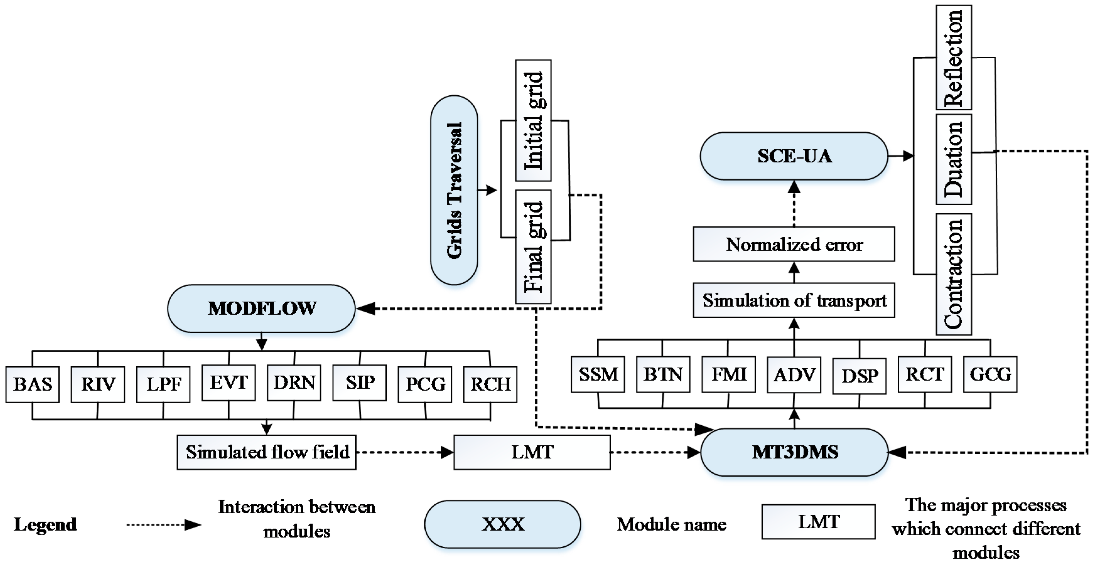
To produce reasonable and efficient identifications for unknown pollution source characteristics based on observation data, our proposed S/O model was built by integrating the Grids Traversal and SCE-UA algorithms into numerical simulators including MT3DMS and MODFLOW. MODFLOW is used for simulating a flow field that serves as an input to simulate pollutant transport process in MT3DMS [36]. The model structure is shown in Figure 1. More detailed descriptions of each module and its interactions with other modules are further discussed in Section 2.2, Section 2.3 and Section 2.4.

2.2. Numerical and Optimization Methods

2.2.1. Governing Equations

Three-dimensional (3D) transient groundwater flow through a heterogeneous, anisotropic, and saturated aquifer can be represented by the following partial differential equation [37]:

$$\frac{\partial }{\partial x}\left(K_{xx}\frac{\partial h}{\partial x}\right)+\frac{\partial }{\partial y}\left(K_{yy}\frac{\partial h}{\partial y}\right)+\frac{\partial }{\partial z}\left(K_{zz}\frac{\partial h}{\partial z}\right)+W=S_s\frac{\partial h}{\partial t}$$

(1)

where K_xx, K_yy, and K_zz are hydraulic conductivities along the x, y, and z directions, respectively, which are assumed to be parallel to the principle flow directions (L T⁻¹), h is the potentiometric head (L), W is volumetric flux per unit volume of aquifer representing fluid sources (positive) and sinks (negative) (T⁻¹), S_s is the specific storage of the porous media (L⁻¹), and t is the time step (T). The governing Equation (1) along with the hydrogeological boundary and initial conditions can simulate transient 3D ground-water flow in a heterogeneous and anisotropic medium.

Pollutant transport through the heterogeneous and saturated aquifer is governed by the 3D advection-dispersion equation [36,38]:

$$\frac{\partial }{\partial x_i}\left(\theta D_{ij}\frac{\partial C^k}{\partial x_j}\right)-\frac{\partial }{\partial x_i}\left(\theta v_i{C}^k\right)+q_S{C}_s^k+{\displaystyle \sum R_n}=\frac{\partial (\theta C^k)}{\partial t}$$

(2)

where θ is the dimensionless porosity; C^k is the concentrations of species k (ML⁻³); D_i,j is the hydrodynamic dispersion coefficient tensor (L² T⁻¹); v_i is the seepage or linear pore water velocity (L T⁻¹), v_i = q_i/θ, q_i is the specific discharge or Darcy flux, q_S is the volumetric flow rate per unit volume of aquifer representing fluid sources (positive) and sinks (negative), T⁻¹; C^k_S is the concentration of the source or sink flux for species k, ML⁻³; and ∑Rn are chemical reaction terms, ML⁻³ T⁻¹.

2.2.2. SCE-UA Algorithm

The Shuffled Complex Evolution algorithm (SCE-UA) is a generalized global searching optimization algorithm that was originally developed by Qingyun Duan of the University of Arizona [39]. The SCE-UA algorithm combines complex procedures with competition evolution theory, concepts of controlled random search, the complex shuffling method, and downhill simplex procedures to obtain a global optimal estimation. It has been used in many hydrological inverse models for determining unknown hydrological parameters [18,19,40,41,42,43,44,45]. Previous studies have indicated that the SCE-UA algorithm is able to accurately identify the appropriate values for model parameters. In most cases, the SCE-UA algorithm can robustly and rapidly achieve a satisfactory result with a global minimum error.

2.3. Grids Traversal Algorithm

Accurate determination of pollution source locations is crucial for groundwater pollution treatment. However, in most cases, pollution source locations are often unknown. A common method for addressing this is to manually predefine an area covering all possible pollution sources based on field investigation. Moreover, the complexity of identification would be increased substantially with the increasing number of potential pollution sources. For example, if the predefined area covers 16 grids and only one pollution location is existent, in theory, we can possibly have 16 combinations of locations. However, if there are two potential pollution source locations in this area, then 120 combinations are theoretically possible with regard to contaminant source locations.

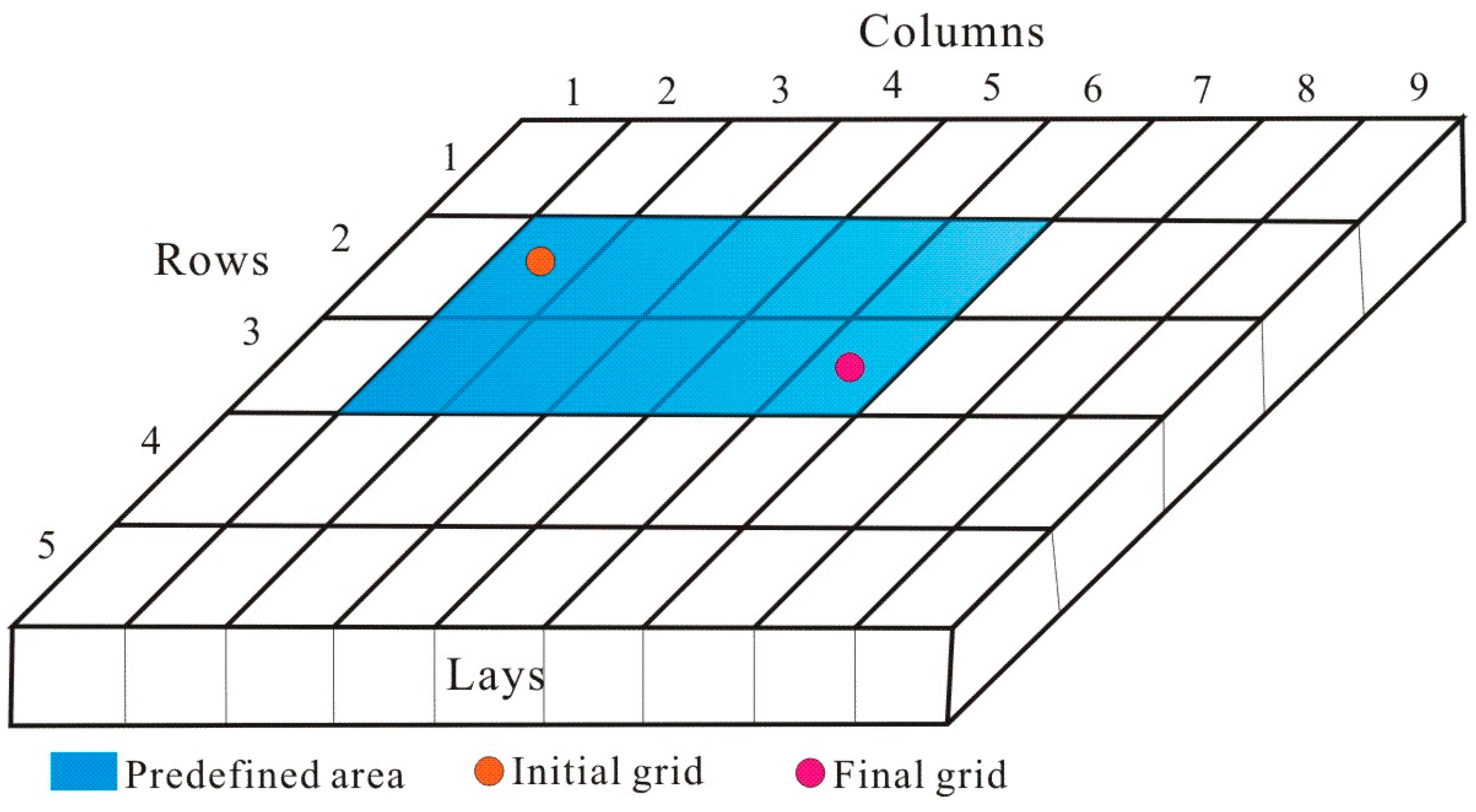
In this study, we proposed to use the Grids Traversal algorithm, which can automatically search all possible combinations of pollution source locations. In the framework of the Grids Traversal algorithm, the range of the predefined area is defined by a grid index of two endpoints, as shown in Figure 2, the initial and final grids. 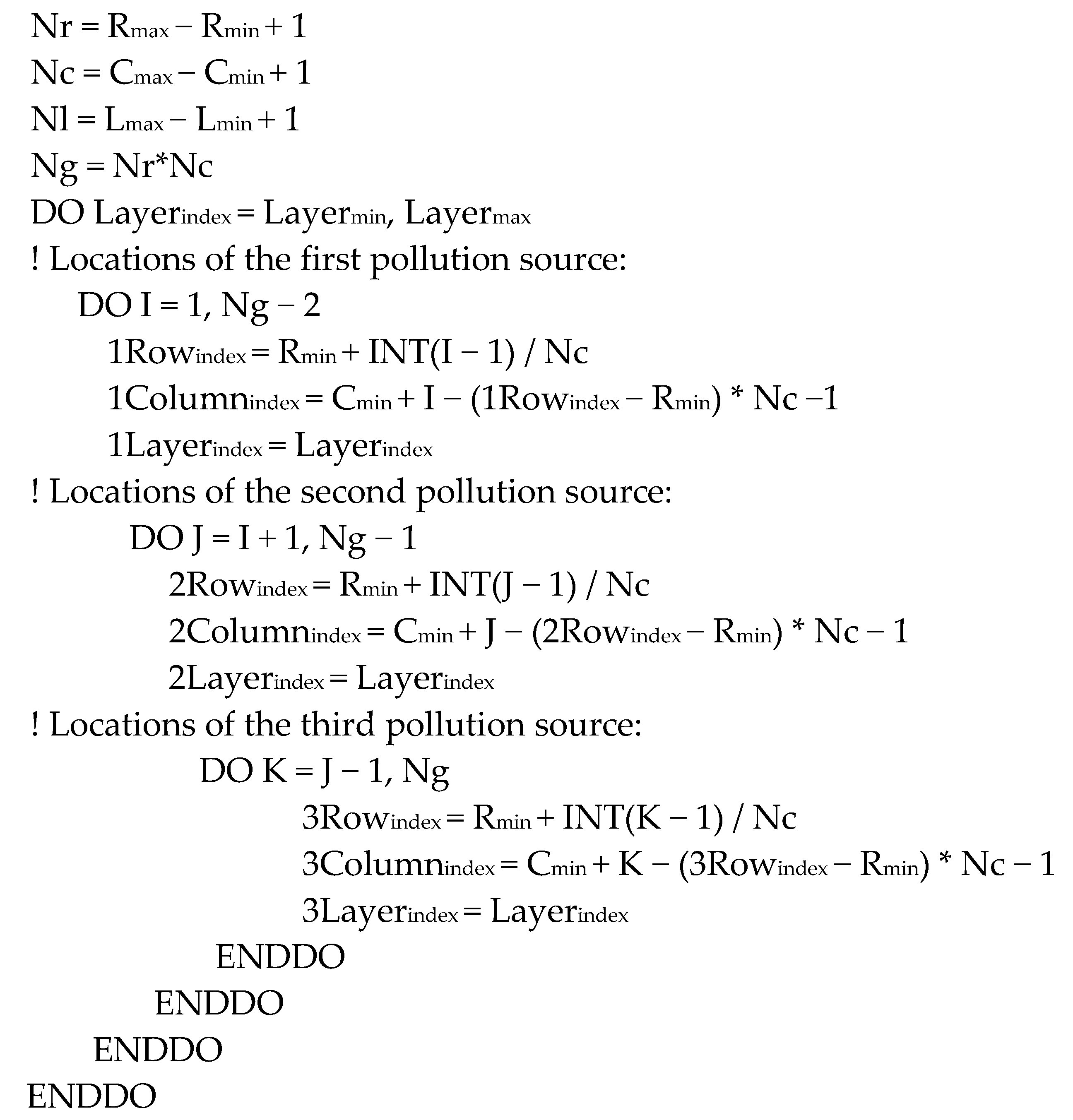The initial grid defines the lower bounds of the row, column, and layer of the predefined area labeled as R_min, C_min, and L_min, respectively; and the final grid defines the upper bounds of the row, column, and layer of the predefined area denoted as C_max, R_max, and L_max, respectively. The S/O model requires the inputs for the lower and upper bounds and the number of potential pollution source locations. All possible combinations of pollution source locations can be automatically searched by the Grids Traversal algorithm within the area bounded by the initial and final grids. The search process was performed though a computer program written by FORTRAN internally coupled with the S/O model (Figure 3). For example, if the predefined area covers three grids which are marked as 1, 2, and 3 and two source locations are existent, the Grids Traversal algorithm would search step-by-step, i.e., (1, 2), (1, 3), and (2, 3), until all possible pollution source locations have been fully searched. For a transient flow, the Grids Traversal algorithm will search all possible pollution source locations at all time steps throughout the running time.

2.4. The S/O Model

2.4.1. Residual Error (RE)

The identification of unknown groundwater pollution source characteristics aims at minimizing the residual error (RE), which is the sum of absolute differences between the simulated and observed concentrations divided by the observed concentration. The residual error is mathematically described as [46,47]:

$$R{E}^t=\min \left[{\displaystyle \sum _{m1=1}^{Nm1}|\frac{Csi{m}_{m1}^t-Cob{s}_{m1}^t}{Cob{s}_{m1}^t}}|\times 100\right]$$

(3)

Subject to

$$C=f(Q)$$

(4)

$$Q^l\le Q\le Q^u$$

(5)

where t represents the tth stress period; Nm1 is the total number of observation locations; Csim^t_m1 is the simulated concentration at the m1th observation location of the tth stress period; Cobs^t_m1 is the observed concentration at the m1th observation location of the tth stress period; Q^l and Q^u are the lower and upper bounds representing possible ranges for the concentration variables Q of pollution sources, respectively; and f(Q) is a function transforming the concentration variables Q of pollution sources into concentration variables C of observation locations via the groundwater flow and transport models.

If the RE value is zero, the identified pollution locations and concentrations perfectly match the observational data, but in reality the RE is always greater than 0 due to the errors induced by simulation and observation. Essentially, a smaller RE suggests a better match between the simulated concentration and the observed concentrations.

2.4.2. Normalized Deviation (ND)

The performance of the S/O model can be better measured by a normalized difference between the actual and simulated concentrations of pollution sources, which is defined as:

$$N{D}^t={\displaystyle \sum _{m2=1}^{Nm2}\frac{|Qid{e}_{m2}^t-Qac{t}_{m2}^t|}{Qac{t}_{m2}^t}}\times 100$$

(6)

where Nm2 is the total number of pollution sources; Qide^t_m2 is the identified concentration at the m2th pollution source of the tth stress period; and Qact^t_m2 is the actual concentration at the m2th pollution source of the tth stress period. A smaller ND value represents that the identified source concentrations are closer to the actual values, and thus that the S/O model performs better.

2.4.3. Incorporating Measurement Errors

Identified concentrations would be perturbed by the concentration measurement errors that generally occur in field measurements or laboratory tests. In order to evaluate how sensitive the S/O model is to the measurement errors, an analysis for the S/O model incorporating measurement errors was therefore performed. The perturbed concentration value is defined as follows [48]:

$$Cob{s_{m1}^t}^{\prime }=Cob{s}_{m1}^t+\epsilon r$$

(7)

where $Cob{s_{m1}^t}^{\prime }$ is the perturbed observed concentration at the m1^th observation location of the tth stress period; and $\epsilon r$ is the random error term and can be defined as:

$$\epsilon r=\mathrm{a}\times Cob{s}_{m1}^t$$

(8)

where 0 ≤ a ≤ 1.0. In this study, a varies from 0.05 to 0.3. A larger a indicates a higher level of noise in the data; it is assumed that a <0.15 corresponds to a low noise level; 0.15 ≤ a ≤ 0.25 corresponds to a moderate noise level; and a >0.25 corresponds to a high noise level. Note that a = 0 represents that measurements are free of error.

2.4.4. Linkage of Simulation-Optimization Model

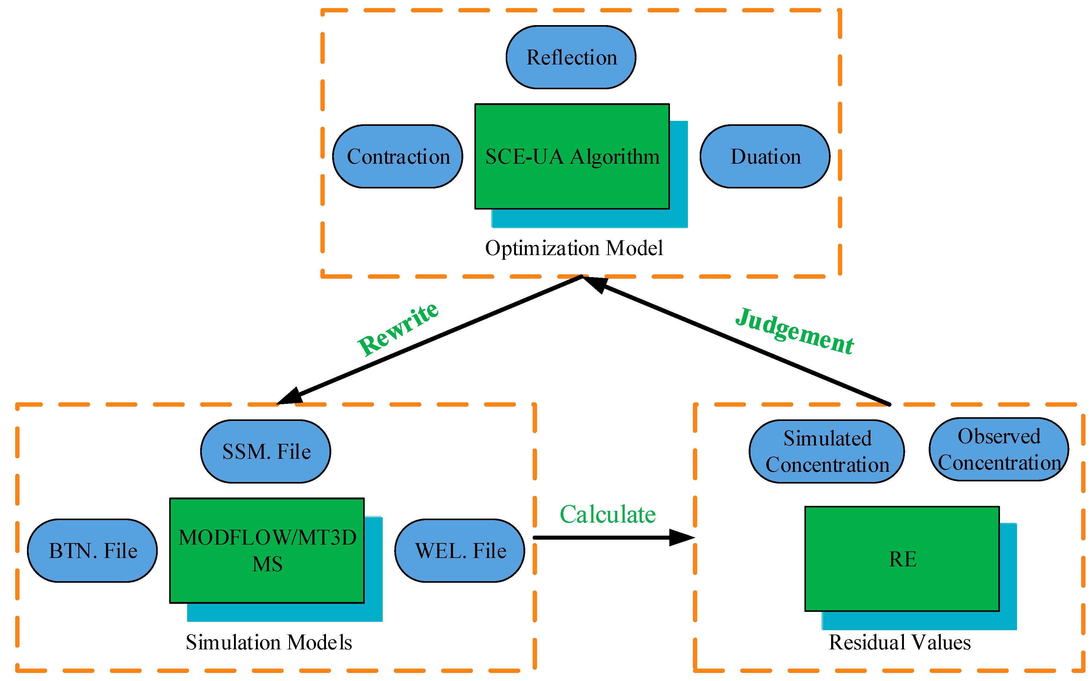
The S/O identification model can be divided into two main sections: simulation and optimization models. The simulation model includes MODFLOW and MT3DMS that were used to simulate the groundwater flow and contaminant transport processes. The optimization model includes the SCE-UA algorithm, which was used to automatically alter the concentrations of pollution sources to better fit the observational dataset. Figure 4 shows the interactions of the simulation and optimization models. The Grids Traversal algorithm mentioned above was incorporated into the S/O model. All of these functions are internally linked by FORTRAN interface programs and can be easily compiled into one execution file. This novel design modifies the way of data exchange from using external files to programming variables, which makes the S/O model feasible to deal with transient flow problems; this can significantly improve the accuracy and efficiency of computation for the inverse problem.

Identification of unknown groundwater pollution source characteristics was performed by four procedures at every stress period: (1) The Grids Traversal algorithm generated new possible pollution source locations; (2) The SCE-UA algorithm and interface program rewrote input files of simulation models, such as .BTN, .SSM, and .WEL, with predefined or updated values; (3) MODFLOW and MT3DMS simulated pollutant concentrations of observation locations with updated concentrations and locations of pollution sources, and then the interface program calculated the RE values; and (4) The SCE-UA algorithm updated pollutant concentrations of pollution sources by three steps (reflection, contraction, and duration) based on RE values. When all possible pollution source locations have been identified, the identification process will move on to the next stress period until all stress periods were implemented. Figure 5 illustrates the identification process of the S/O model.

3. Assessment of the S/O Optimization Model

The performance and robustness of this proposed S/O optimization model was assessed by various combinations of simple and complex situations of three hypothetical scenarios as discussed below.

3.1. Hypothetical Scenarios

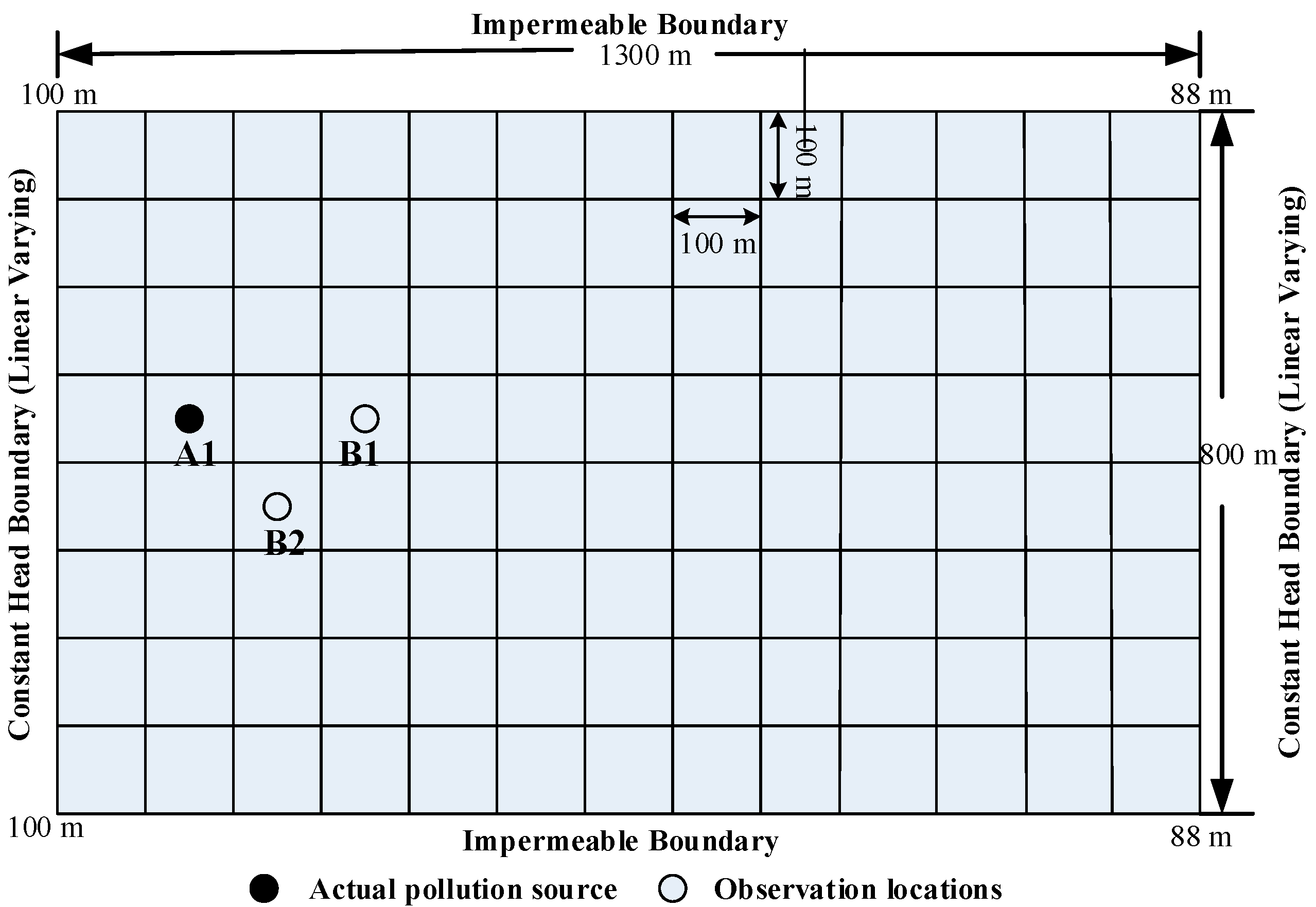
In all hypothetical scenarios, a two-dimensional confined aquifer with a simplified aquifer domain and boundary conditions was considered. This model grid was taken and modified from Datta, Chakrabarty and Dhar [46] and Singh and Datta [49]. The study area was assumed to be homogeneous and isotropic. The plan view is shown in Figure 6. The rectangle aquifer model had dimensions of 1300 m × 800 m and was discretized into square grid blocks with a grid size of 100 m × 100 m. The boundary conditions were specified as constant head = 100 m at west and constant head = 88 m at east, and no-flow was imposed at the upper and lower boundaries.

The parameters of the groundwater flow and transport models are listed in

Table 2. Parameters of the groundwater flow and transport model.

Parameter	Value
Kxx (LT−1)	0.1
Kyy (LT−1)	0.1
△x (L)	100
△y (L)	100
b (L)	80
Di,j (L2 T−1)	40
ε	0.3

. All hydrogeological parameters and flow conditions of the numerical model were simplified to test the proposed S/O model.

The control parameters of the SCE-UA algorithm are given in

Table 3. Input control parameters of SCE-UA algorithm.

Parameter	Value
Generation number	10
Number of points in each complex	3
Number of complex	10
Sample size	30
Number of points in each sub-complex	2
Number of each sub-complex evolution step	5
Ql (mg L−1)	0
Qu (mg L−1)	80

.

Three hypothetical scenarios were designed with varying numbers, locations, and concentrations of pollution sources and observation locations:

(1)

A simple scenario with one pollution source (location is known) and two observation locations under steady-state flow;

(2)

A complex scenario with two potential pollution sources (locations are unknown) and four observation locations under a steady-state flow condition;

(3)

A more complex scenario with two potential pollution sources (locations are unknown) and four observation locations under transient flow conditions with three stress periods.

3.1.1. Scenario 1

Identification with Error-Free Concentration Measurements in Scenario 1

For Scenario 1, one pollution source was considered at A1 (row = 4, column = 1, Q_act1 = 48 mg L⁻¹). Two observation locations were considered respectively at O1 (row = 4, column = 4, C_obs1 = 1.58 × 10⁻⁵ mg L⁻¹) and O2 (row = 5, column = 3, Cobs2 = 1.16 × 10⁻⁵ mg L⁻¹) (Figure 6). The S/O optimization model was able to use the observed concentrations C_obs1 and C_obs2 to correctly identify the concentration Q_act1 of the pollution source. The performance of the S/O model was measured by the normalized deviation (ND) between the identified and actual concentration values. The identified results with different generation numbers are given in

Table 4. Effect of variation in the generation number.

Concentration	Generation Number
	10	20	50
Actual concentration (mg L−1)	48	48	48
Identified concentration (mg L−1)	47.982	47.999	48.002
ND (%)	0.037	0.002	0.005

Note: ND: normalized deviation.

and Figure 7. Note that the concentration values used for graphing in Figure 7 are the optimal results of each generation.

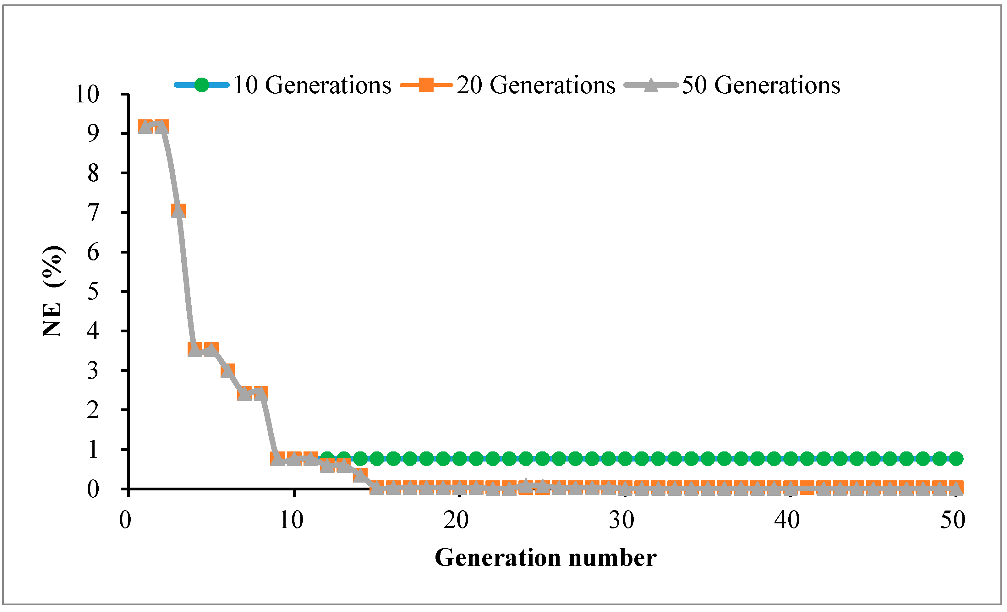
The performance of the S/O optimization model was assessed by using the generation number of 10, 20, and 50. As is shown in Table 4 and Figure 7, ND values with a different generation number were all trivial, which suggested that the identified concentrations robustly matched the imposed concentration. Although the identified concentrations were different from the actual value at the very first iteration, the S/O optimization model was able to eventually reproduce the actual concentration with increasing generation number. Note that an increase in the generation number from 20 to 50 was found to produce only a marginal difference in the identification results but could significantly increase the computational burden.

Identification with Concentration Measurement Errors in Scenario 1

The performance of the S/O optimization model considering concentration measurement errors was assessed and is presented in

Table 5. Identified results with different noise levels.

Noise Levels A	Actual Concentration (mg L−1)	Identified Concentration (mg L−1)	ND (%)
0.05	48	48.009	0.020
0.1	48	50.516	5.242
0.15	48	52.744	9.883
0.2	48	56.557	17.828
0.25	48	59.036	22.991
0.3	48	61.528	28.183

. It was observed that when a low noise level was included in the observational data, the ND is relatively low, ranging from 0.02% to 9.883%; when the noise level was moderate and high, the ND values were relatively high, spanning from 17.828% to 28.183%. These facts indicated that the identified results could be slightly affected by a low noise level but can be pronouncedly affected by moderate and high noise levels. However, the influence of concentration measurement errors could be realistically reduced by (1) more observation locations with (2) more concentration measurements. This is further demonstrated by the following scenarios.

3.1.2. Scenario 2

In many cases, we can hardly access useful information about pollution source locations and concentrations. To evaluate the capability of the S/O optimization model for addressing this kind of issue, a complex scenario with additional pollution sources and observation locations was considered.

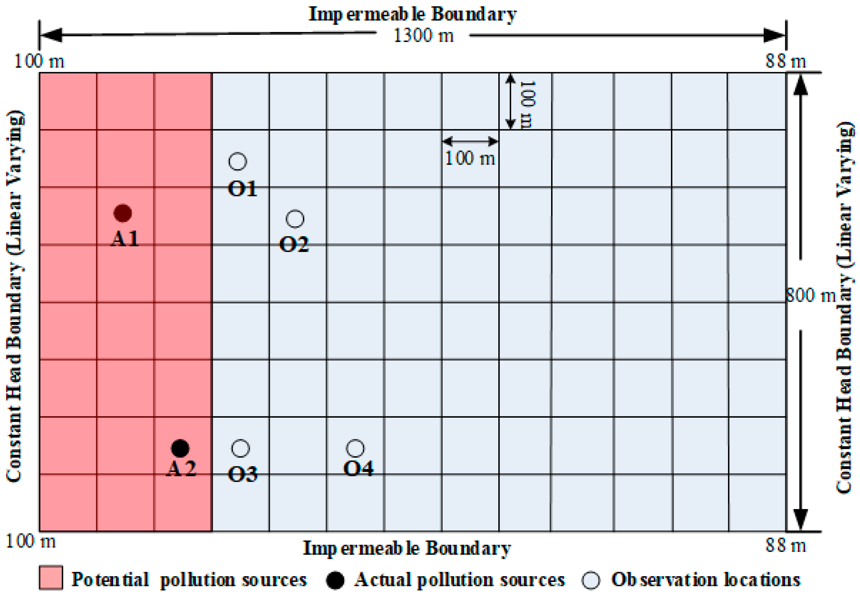
In Scenario 2, it was assumed that there were two pollution sources and that their potential locations were spread over a predefined subarea of 24 grids (covered by red color in Figure 8) of the study area. Therefore, these two pollution sources could be located in any two of the 24 possible grids and a total 276 combinations of locations needed to be searched and identified.

The actual locations of these two pollution sources were assumed to locate in A1 (row = 3, column = 2, Q_act1 = 48 mg L⁻¹) and A2 (row = 7, column = 3, Q_act2 =36 mg L⁻¹), respectively. The four observation locations and their relevant concentrations are O1 (row = 2, column = 4, C_obs1 = 1.13 × 10⁻⁵ mg L⁻¹), O2 (row = 3, column = 5, C_obs2 = 0.17 mg L⁻¹), O3 (row = 7, column = 4, C_obs3 = 3.53 × 10⁻⁶ mg L⁻¹), and O4 (row = 7, column = 6, C_obs4 = 6.46 × 10⁻⁶ mg L⁻¹), respectively.

A large number of pollution source locations have been determined, but we only show the most satisfying results with smaller ND values (

Table 6. Comparison of actual and identified pollution sources characteristics for generation = 10.

Results No.	Locations of Pollution Sources			Concentrations of Pollution Sources		ND (%)
		Actual (mg L−1)	Identified (mg L−1)	Actual (mg L−1)	Identified (mg L−1)
1	A1	(3, 2)	(3, 2)	48	47.950	0.323
	A2	(7, 3)	(7, 3)	36	35.805
2	A1	(3, 2)	(3, 2)	48	48.067	0.570
	A2	(7, 3)	(7, 3)	36	36.360
3	A1	(3, 2)	(3, 2)	48	49.561	1.945
	A2	(7, 3)	(7, 3)	36	35.770
4	A1	(3, 2)	(3, 2)	48	47.996	8.236
	A2	(7, 3)	(8, 1)	36	30.073
5	A1	(3, 2)	(2, 1)	48	47.99	47.108
	A2	(7, 3)	(7, 3)	36	69.91
6	A1	(3, 2)	(8, 2)	48	2.120	90.765
	A2	(7, 3)	(8, 3)	36	66.941

). The pollution source locations have been correctly identified from the 276 possible locations. The minimum ND value was 0.323%; this showed that both locations and concentrations matched well with the actual values. The best identified concentrations were 47.95 mg L⁻¹ and 35.81 mg L⁻¹, respectively, which is identical to the actual concentrations 48 mg L⁻¹ and 36 mg L⁻¹. Note that when the identified locations were correctly located, the ND values varied from 0.323% to 1.945% with satisfactory estimated concentrations; when the identified locations were missed, the ND values varied from 8.236% to 90.765% and the identified concentrations were very different from the imposed concentrations. The above suggests that a correct determination of pollution source locations is necessary for further correctly identifying the pollution source concentrations.

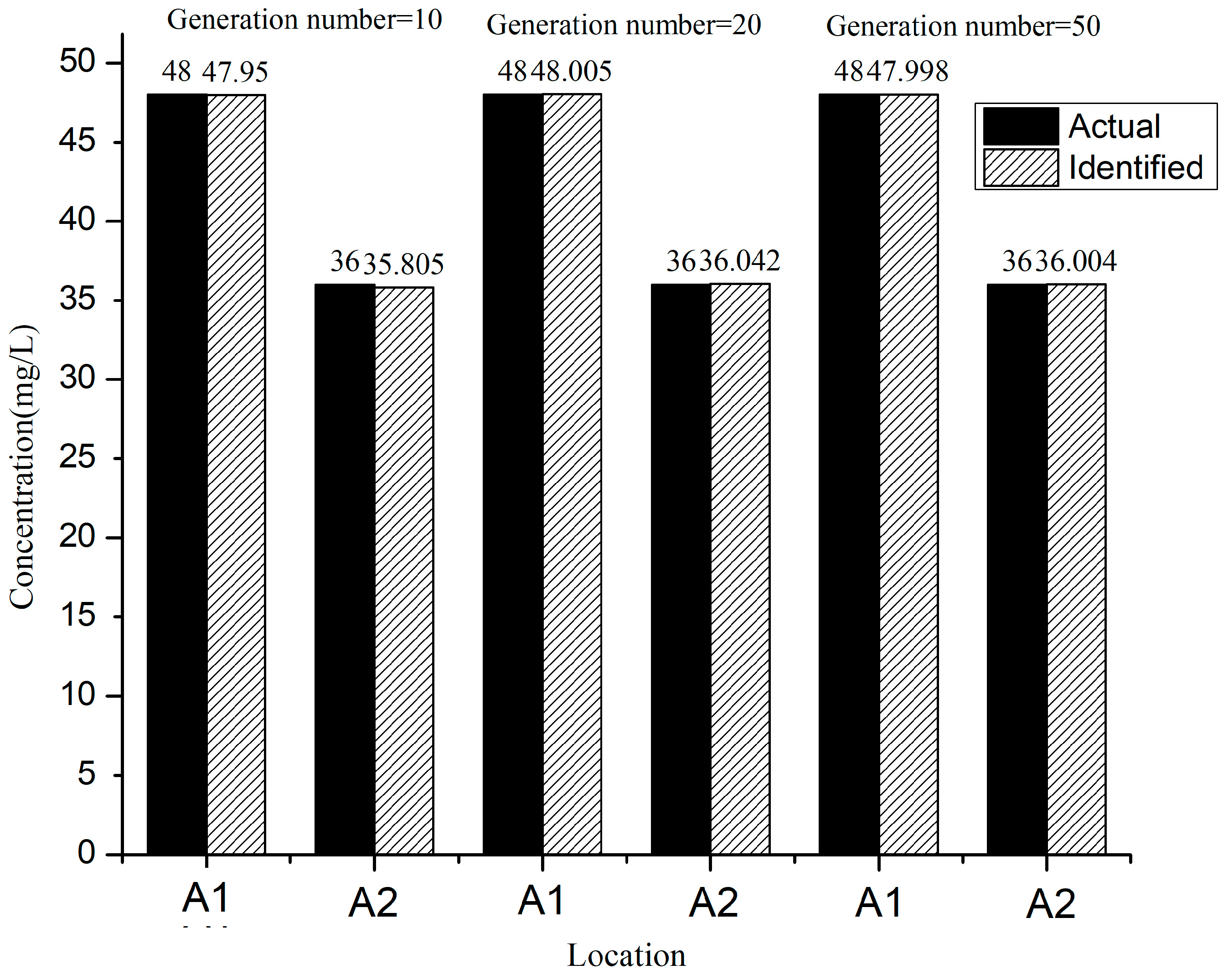
The effect of variation in generation number was additionally analyzed. The optimal identified results for generation numbers 10, 20, and 50 were both lower than 1%, which demonstrates that the S/O model is robust for inversely capturing the contaminant concentrations and locations (

Table 7. Effect of variation in generation number.

Generation	Locations of Pollution Sources			Concentrations of Pollution Sources		ND (%)
	Title	Actual	Identified	Actual (mg L−1)	Identified (mg L−1)
10	A1	(3, 2)	(3, 2)	48	47.950	0.323
	A2	(7, 3)	(7, 3)	36	35.805
20	A1	(3, 2)	(3, 2)	48	48.005	0.064
	A2	(7, 3)	(7, 3)	36	36.042
50	A1	(3, 2)	(3, 2)	48	47.998	0.008
	A2	(7, 3)	(7, 3)	36	36.004

and Figure 9). The identified results indicate that ND values could be reduced by increasing the number of generations, but with only a negligible improvement after the 10th generation.

3.1.3. Scenario 3

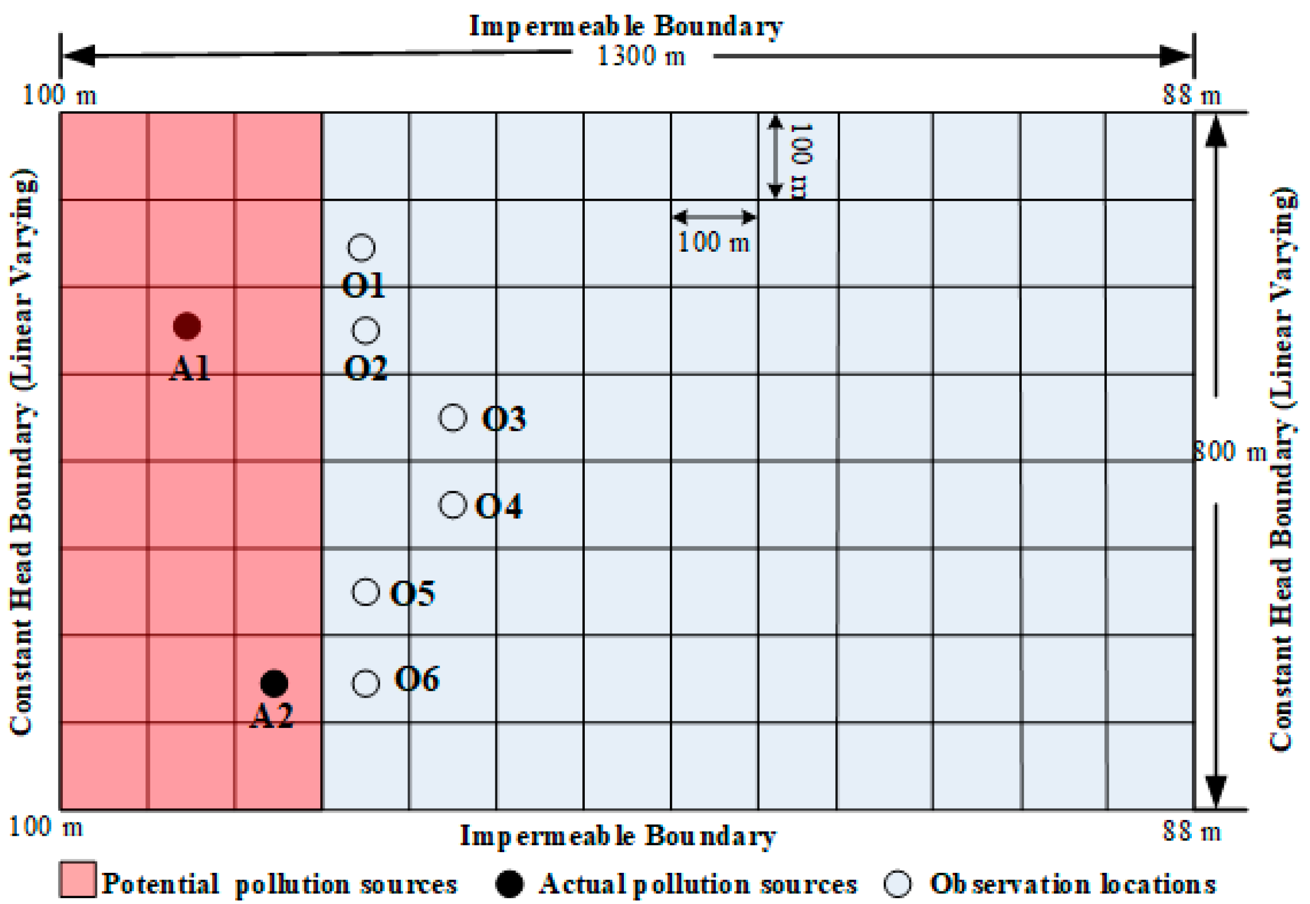
This scenario represents the most real-world application, where the pollutant concentrations of pollution sources are varying at different stress periods. Therefore, a more complex hypothetical scenario was designed for a transient flow with a 3-year time domain. The temporal space had three stress periods; each period was one year that was further divided into 10 equal time steps.

In this hypothetical scenario, there were two pollution sources that potentially spread over a predefined subarea comprising 24 grids (covered by red color in Figure 10). In principle, these two pollution sources may be located in any two of the 24 grid locations and a total of 276 possible combinations of locations needed to be searched and identified at each stress period. The actual locations of these two pollution sources were set to be located in A1 (row = 3, column = 2) and A2 (row = 7, column = 3). Six observation locations were considered and located at O1 (row = 2, column = 4), O2 (row = 3, column = 4), O3 (row = 4, column = 5), O4 (row = 5, column = 5), O5 (row = 6, column = 4), and O6 (row= 7, column = 4), respectively. The concentrations of these two pollution sources differed at each stress period. The imposed concentrations and locations of actual pollution sources (Q_act) and observation location (C_obs) at each stress period are listed in

Table 8. Concentrations and locations of actual pollution sources and observation locations for each stress period.

Title	Locations	Stress Period 1 (mg L−1)	Stress Period 2 (mg L−1)	Stress Period 3 (mg L−1)
A1	(3, 2)	48	36	24
A2	(7, 3)	36	0	24
O1	(2, 4)	8.7 × 10−6	1.23 × 10−4	5.57 × 10−4
O2	(3, 4)	6.21 × 10−4	4.34 × 10−3	1.28 × 10−2
O3	(4, 5)	2.88 × 10−8	7.18 × 10−7	5.04 × 10−6
O4	(5, 5)	7.13 × 10−7	1.67 × 10−5	9.77 × 10−5
O5	(6, 4)	1.38 × 10−2	8.63 × 10−2	0.21
O6	(7, 4)	0.47	1.16	1.85

.

For a transient flow problem, the identification of the current stress period was based on the identified results of the previous stress period. For example, the identification of the first stress period was solved by treating the flow system as at steady-state. During the second stress period, the S/O optimization model directly used the identified results of the first stress period as input that serves as an initial guess for the second stress period. The same procedure is applied until the end of simulation time to fully accomplish the whole identification process. Note that the identified results of the current stress period would be significantly affected by the identified results of the previous stress period. Therefore, the ND value (i.e., errors) would accumulate with the increasing stress periods.

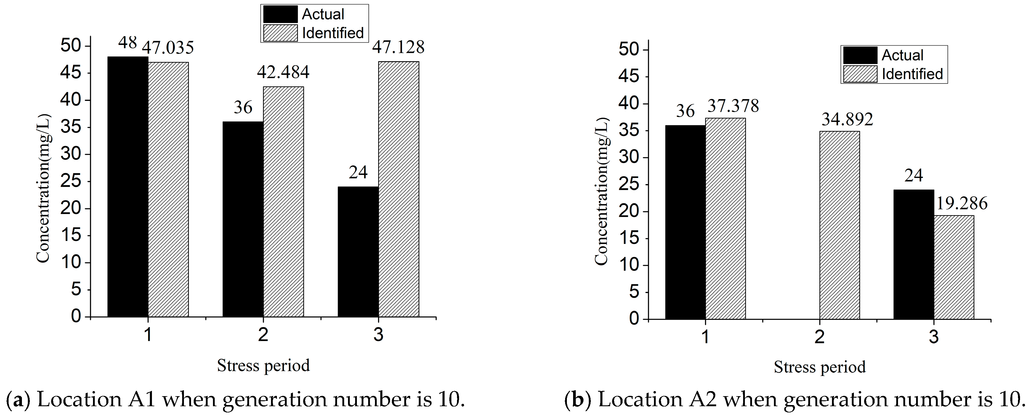
The optimal identification results of each stress period are shown in

Table 9. Comparison of actual and identified characteristics when the generation number is 10.

Stress Period No.	Locations			Concentrations		ND (%)
		Actual	Identified	Actual (mg L−1)	Identified (mg L−1)
1	A1	(3, 2)	(3, 2)	48	47.035	2.91
	A2	(7, 3)	(7, 3)	36	37.378
2	A1	(3, 2)	(3, 2)	36	42.484	-
	A2	(7, 3)	(7, 1)	0	34.892
3	A1	(3, 2)	(8, 2)	24	47.128	58
	A2	(7, 3)	(8, 3)	24	19.286

and Figure 11 when the generation number was 10. The ND value is 2.91 at the first stress period, which was acceptable (Table 9), but the identified location and concentration does not match well with the actual values at the second and the third stress periods; the ND value increased up to 58 at the end of the third stress period. This indicates that satisfactory results cannot be inversely resolved if the generation number is 10.

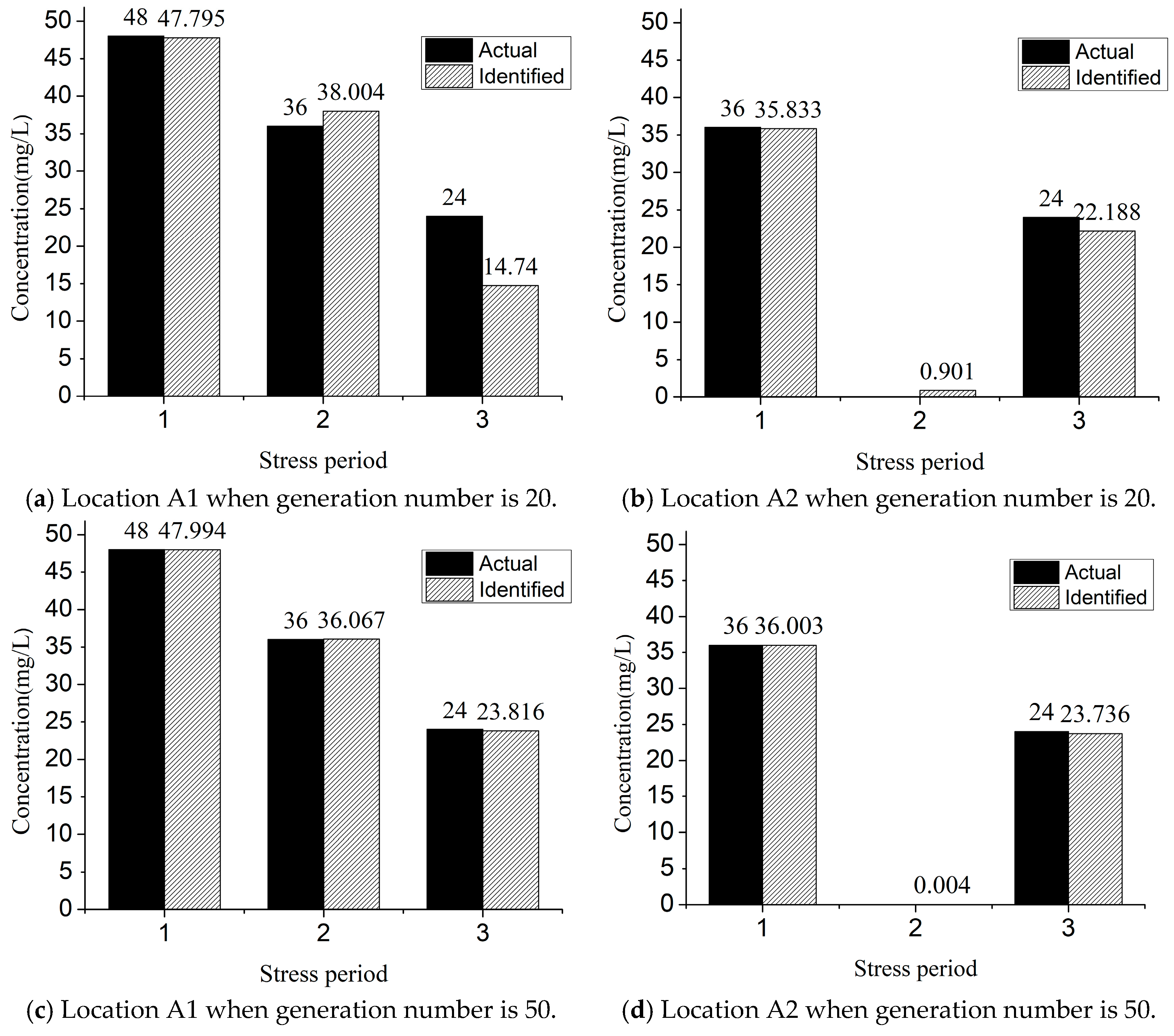
When the generation number was set to be 20, only the first and the second stress periods can obtain acceptable results (

Table 10. Comparison of actual and identified characteristics when the generation number is 20 and 50.

Generation	Stress Period No.	Location			Concentrations		ND (%)
			Actual	Identified	Actual (mg L−1)	Identified (mg L−1)
20	1	A1	(3, 2)	(3, 2)	48	47.795	0.45
		A2	(7, 3)	(7, 3)	36	35.833
	2	A1	(3, 2)	(3, 2)	36	38.004	-
		A2	(7, 3)	(7, 3)	0	0.901
	3	A1	(3, 2)	(3, 2)	24	14.740	23
		A2	(7, 3)	(7, 3)	24	22.188
50	1	A1	(3, 2)	(3, 2)	48	47.994	6 × 10−5
		A2	(7, 3)	(7, 3)	36	36.003
	2	A1	(3, 2)	(3, 2)	36	36.067	-
		A2	(7, 3)	(7, 3)	0	0.004
	3	A1	(3, 2)	(3, 2)	24	23.816	0.93
		A2	(7, 3)	(7, 3)	24	23.736

and Figure 12). However, if the generation number was further increased to 50, the S/O model can produce satisfactory results at all three stress periods (Table 10 and Figure 12).

The results from the above with different generation numbers suggests that, when the situation refers to transient flow identification, a larger generation number is required to achieve satisfactory results than that for the steady state cases, since the identified errors would keep accumulating throughout the whole identification process. Moreover, if the identification problem has more stress periods, a large generation number is needed to obtain more accurate results.

3.2. Comparison with an ANN-Based Model

The performance of the S/O identification model was further assessed by comparing it to an artificial neural network (ANN) model [11]. In the ANN-based model, the ANN optimization algorithm does not explicitly link with physical simulation models, such as MODFLOW and MT3DMS. However, the solutions of the flow and transport models are still required for the training of the ANN. Therefore, the simulated results produced by the physical simulation model are externally added to the training process of the ANN, which makes the performance of the ANN-based model less efficient. The identified results using the proposed S/O model are comparatively more efficient than those using the ANN-based model (

Table 11. Comparison of identification errors using the proposed S/O model and the artificial neural network (ANN)-based model.

Stress Period No.	S/O Model		ANN-Based Model
	Generation Number	ND (%)	Generation Number	ND (%)
1	50	6 × 10−5	50	0.24
2	50	-	50	-
3	50	0.93	50	10.38

). The ND value was 0.24 in the first stress period obtained using the ANN-based model. However, the ND value increased to 10.38 in the third stress period, suggesting that the identified results were very different from the actual dataset. This is partly because the ANN-based model requires numerous data for sample training; hence, a larger generation number was needed to achieve a better solution.

4. Conclusions

In this study, a SCE-UA-based simulation-optimization (S/O) model and a Grids Traversal algorithm were introduced to address the inverse problem of identifying groundwater pollution sources. This proposed S/O model is applicable for scenarios where there is little information about the starting release time, locations, and concentrations. Moreover, the S/O model can handle multiple sources having different source activities in each stress period with a transient flow field. The case studies showed that the S/O model can effectively and accurately identify unknown groundwater pollution, while the artificial neural network (ANN) model is less computationally efficient. The performance of the S/O model can be improved by increasing the number of generations, but this only produces marginal improvement after reaching the threshold generation number while increasing computational cost. When solving a transient flow inverse problem, a larger generation number is needed for reducing the accumulation of identification errors from the previous stress periods.

However, it is still a challenge for the S/O model and other existing source identification models to reliably handle a real-world case. This is because of following reasons. First, in the S/O model, we use MODFLOW and MT3DMS to simulate groundwater flow and contaminant transport processes. The performance of the S/O model depends on how closely the physically based simulation model represents the complex aquifer properties and relevant transport behavior. Specifically, groundwater systems are typically heterogeneous and anisotropic in terms of aquifer properties (i.e., hydraulic conductivity). Moreover, boundary conditions typically vary greatly in both space and time. Therefore, the accurate characterization of a reliable physically based model itself presents a challenge with limited field data. Second, there are almost infinite possibilities of contaminant release activities in reality. For example, the releasing time and durations of the sources are normally unknown and the source location can be potentially everywhere in the study area. Although the proposed Grids Traversal algorithm can automatically search all possible combinations of pollution source locations, the absence of exact prior information, including the timing of release and the duration of the contaminant source, makes the S/O model and other existing source identification models less efficient, and also makes it sometimes impossible to complete the inverse problem. Third, although the inverse models are viable to identify all possibilities with great computational efficiency (i.e., the S/O model proposed here), a complex real-world case may require hundreds of thousands of simulation runs. This consequently induces an intensive computational burden and elongated execution time; this needs enormous efforts and usually it is unaffordable to do so.

Overall, this study developed a novel S/O optimization model to resolve unknown groundwater pollution problems. However, further developments are still necessary to relax the limitations of the S/O model to solve more complex problems. Advanced analysis and computation techniques, reduced-order model techniques, including parallel computing techniques, parameter regularization, and new optimization algorithms, would be useful to save computational cost and facilitate future model development. Last but not least, a user-friendly operational software package can broaden the model’s applications. More case studies are needed to further demonstrate its applicability.

References

- Li, W.; Wang, M.Y.; Liu, L.Y.; Yan, Y. Assessment of long-term evolution of groundwater hydrochemical characteristics using multiple approaches: A case study in cangzhou, northern China. Water 2015, 7, 1109–1128. [Google Scholar] [CrossRef]
- Hu, L. Surrogate models for sub-region groundwater management in the beijing plain, China. Water 2017, 9, 766. [Google Scholar] [CrossRef]
- Wei, X.H. China’s groundwater pollution control difficulties and countermeasures. Energy Energy Conserv. 2013, 8, 67–68. (In Chinese) [Google Scholar]
- Yang, M.; Fei, Y.; Ju, Y.; Ma, Z.; Li, H. Health risk assessment of groundwater pollution—A case study of typical city in north china plain. J. Earth Sci. 2012, 23, 335–348. [Google Scholar] [CrossRef]
- Li, X.; Li, G.; Zhang, Y. Identifying major factors affecting groundwater change in the north china plain with grey relational analysis. Water 2014, 6, 1581–1600. [Google Scholar] [CrossRef]
- Wang, H.; Cai, Y.; Tan, Q.; Zeng, Y. Evaluation of groundwater remediation technologies based on fuzzy multi-criteria decision analysis approaches. Water 2017, 9, 443. [Google Scholar] [CrossRef]
- Atmadja, J.; Bagtzoglou, A.C. State of the art report on mathematical methods for groundwater pollution source identification. Environ. Forensics 2001, 2, 205–214. [Google Scholar] [CrossRef]
- Amirabdollahian, M.; Datta, B. Identification of contaminant source characteristics and monitoring network design in groundwater aquifers: An overview. J. Environ. Prot. 2013, 4, 26–41. [Google Scholar] [CrossRef]
- Prakash, O.; Datta, B. Optimal monitoring network design for efficient identification of unknown groundwater pollution sources. Int. J. Geomate 2014, 23, 2031–2049. [Google Scholar] [CrossRef]
- Gorelick, S.M.; Evans, B.; Remson, I. Identifying sources of groundwater pollution: An optimization approach. Water Resour. Res. 1983, 19, 117–118. [Google Scholar] [CrossRef]
- Foddis, M.L.; Ackerer, P.; Montisci, A.; Uras, G. Ann-based approach for the estimation of aquifer pollutant source behaviour. Water Sci. Technol. Water Supply 2015, 15, 1285–1294. [Google Scholar] [CrossRef]
- Higuchi, T.; Igarashi, G.; Tohjima, Y.; Wakita, H. Time series analysis of groundwater radon using stochastic differential equations. J. Phys. Earth 2009, 43, 117–130. [Google Scholar] [CrossRef]
- Jha, M.; Datta, B. Three-dimensional groundwater contamination source identification using adaptive simulated annealing. J. Hydrol. Eng. 2013, 18, 307–317. [Google Scholar] [CrossRef]
- Majdalani, S.; Ackerer, P. Identification of groundwater parameters using an adaptative multiscale method. Ground Water 2011, 49, 548–559. [Google Scholar] [CrossRef] [PubMed]
- Li, L.; Zhou, H.; Franssen, H.J.H.; Gómezhernández, J.J. Groundwater flow inverse modeling in non-multigaussian media: Performance assessment of the normal-score ensemble kalman filter. Hydrol. Earth Syst. Sci. 2012, 8, 6749–6788. [Google Scholar] [CrossRef]
- Li, Z.; Mao, X. Global multiquadric collocation method for groundwater contaminant source identification. Environ. Model. Softw. 2011, 26, 1611–1621. [Google Scholar] [CrossRef]
- Hosseini, A.H.; Deutsch, C.V.; Mendoza, C.A.; Biggar, K.W. Inverse modeling for characterization of uncertainty in transport parameters under uncertainty of source geometry in heterogeneous aquifers. J. Hydrol. 2011, 405, 402–416. [Google Scholar] [CrossRef]
- Cooper, V.A.; Nguyen, V.T.V.; Nicell, J.A. Evaluation of global optimization methods for conceptual rainfall-runoff model calibration. Water Sci. Technol. 1997, 36, 53–60. [Google Scholar]
- Kuczera, G. Efficient subspace probabilistic parameter optimization for catchment models. Water Resour. Res. 1997, 33, 177–185. [Google Scholar] [CrossRef]
- Jeon, J.H.; Park, C.G.; Engel, B.A. Comparison of performance between genetic algorithm and sce-ua for calibration of scs-cn surface runoff simulation. Water 2014, 6, 3433–3456. [Google Scholar] [CrossRef]
- Khakbaz, B.; Imam, B.; Hsu, K.; Sorooshian, S. From lumped to distributed via semi-distributed: Calibration strategies for semi-distributed hydrologic models. J. Hydrol. 2012, 418–419, 61–77. [Google Scholar] [CrossRef]
- Jie, C.; Brissette, F.P.; Annie, P.; Robert, L. Overall uncertainty study of the hydrological impacts of climate change for a canadian watershed. Water Resour. Res. 2011, 47, 1–16. [Google Scholar]
- Jeon, J.H.; Lim, K.J.; Engel, B.A. Regional calibration of scs-cn l-thia model:Application for ungauged basins. Water 2014, 6, 1339–1359. [Google Scholar] [CrossRef]
- Huijuna, X.U.; Chen, Y.; Zeng, B.; Jinxianga, H.E.; Liao, Z. Application of sce-ua algorithm to parameter optimization of liuxihe model. Trop. Geogr. 2012, 32, 32–37. [Google Scholar]
- Song, X.M.; Zhan, C.S.; Xia, J. Integration of a statistical emulator approach with the sce-ua method for parameter optimization of a hydrological model. Chin. Sci. Bull. 2012, 57, 3397–3403. [Google Scholar] [CrossRef]
- Chu, J.; Peng, Y.; Ding, W.; Li, Y. A heuristic dynamically dimensioned search with sensitivity information (hdds-s) and application to river basin management. Water 2015, 7, 2214–2238. [Google Scholar] [CrossRef]
- Hong, N.; Hama, T.; Kitajima, T.; Aqili, S.W.; Huang, X.; Wei, Q.; Kawagoshi, Y. Simulation of groundwater levels using tank model with consideration of mixed hydrological structure in kumamoto city. J. Water Environ. Technol. 2015, 13, 313–324. [Google Scholar] [CrossRef]
- Aqili, S.W.; Hong, N.; Hama, T.; Suenaga, Y.; Kawagoshi, Y. Application of modified tank model to simulate groundwater level fluctuations in kabul basin, afghanistan. J. Water Environ. Technol. 2016, 14, 57–66. [Google Scholar] [CrossRef]
- Kan, G.; He, X.; Ding, L.; Li, J.; Liang, K.; Hong, Y. A heterogeneous computing accelerated sce-ua global optimization method using openmp, opencl, cuda, and openacc. Water Sci. Technol. 2017, 76, 1640–1651. [Google Scholar] [CrossRef] [PubMed]
- Ayvaz, M.T.; Elçi, A. A groundwater management tool for solving the pumping cost minimization problem for the tahtali watershed (izmir-turkey) using hybrid hs-solver optimization algorithm. J. Hydrol. 2013, 478, 63–76. [Google Scholar] [CrossRef]
- Ferket, B.V.A.; Samain, B.; Pauwels, V.R.N. Internal validation of conceptual rainfall–runoff models using baseflow separation. J. Hydrol. 2010, 381, 158–173. [Google Scholar] [CrossRef]
- Xie, Z.; Yuan, X. Prediction of water table under stream–aquifer interactions over an arid region. Hydrol. Process. 2010, 24, 160–169. [Google Scholar] [CrossRef]
- Barron, O.; Crosbie, R.; Dawes, W.; Pollock, D.; Charles, S.; Mpelasoka, F.; Aryal, S.; Donn, M.; Wurcker, B. The impact of climate change on groundwater resources: The climate sensitivity of groundwater recharge in australia. Dalton Trans. 2010, 43, 11959–11972. [Google Scholar]
- Simpson, S.C.; Meixner, T.; Hogan, J.F. The role of flood size and duration on streamflow and riparian groundwater composition in a semi-arid basin. J. Hydrol. 2013, 488, 126–135. [Google Scholar] [CrossRef]
- Zhang, Y.; Shao, Q.; Zhang, S.; Zhai, X.; She, D. Multi-metric calibration of hydrological model to capture overall flow regimes. J. Hydrol. 2016, 539, 525–538. [Google Scholar] [CrossRef]
- Zheng, C.; Wang, P.P. Mt3dms: A modular three-dimensional multispecies transport model for simulation of advection, dispersion, and chemical reactions of contaminants in groundwater systems; documentation and user’s guide. AJR Am. J. Roentgenol. 1999, 169, 1196–1197. [Google Scholar]
- Harbaugh, A.W. Modflow-2005, the US Geological Survey Modular Groundwater Model—The Groundwater Flow Process; Center for Integrated Data Analytics Wisconsin Science Center: Reston, VA, USA, 2005.
- Bear, J. Dynamics of Fluids in Porous Media; American Elsevier Pub. Co.: Atlanta, GA, USA, 1972; pp. 174–175. [Google Scholar]
- Duan, Q. A global optimization strategy for efficient and effective calibration of hydrologic models. Int. Arch. Allergy Appl. Immunol. 1991, 86, 176–182. [Google Scholar]
- Duan, Q.; Sorooshian, S.; Gupta, V. Effective and efficient global optimization for conceptual rainfall-runoff models. Water Resour. Res. 1992, 28, 1015–1031. [Google Scholar] [CrossRef]
- Duan, Q.; Sorooshian, S.; Gupta, V.K. Optimal use of the sce-ua global optimization method for calibrating watershed models. J. Hydrol. 1994, 158, 265–284. [Google Scholar] [CrossRef]
- Sorooshian, S.; Duan, Q.; Gupta, V.K. Calibration of rainfall-runoff models: Application of global optimization to the sacramento soil moisture accounting model. Water Resour. Res. 1993, 29, 1185–1194. [Google Scholar] [CrossRef]
- Dong, J.R. Optimal scheduling of hydrothermal system with network and ramping via sce-ua method. Open Cybern. Syst. J. 2015, 7, 55–64. [Google Scholar] [CrossRef]
- Thyer, M.; Kuczera, G.; Bates, B.C. Probabilistic optimization for conceptual rainfall-runoff models: A comparison of the shuffled complex evolution and simulated annealing algorithms. Water Resour. Res. 1999, 35, 767–773. [Google Scholar] [CrossRef] [Green Version]
- Iden, S.C.; Durner, W. Free-form estimation of the unsaturated soil hydraulic properties by inverse modeling using global optimization. Water Resour. Res. 2007, 43, 2217–2221. [Google Scholar] [CrossRef]
- Datta, B.; Chakrabarty, D.; Dhar, A. Identification of unknown groundwater pollution sources using classical optimization with linked simulation. J. Hydro-Environ. Res. 2011, 5, 25–36. [Google Scholar] [CrossRef]
- Jha, M.; Datta, B. Application of Simulated Annealing in Water Resources Management: Optimal Solution of Groundwater Contamination Source Characterization Problem and Monitoring Network Design Problems. In Proceedings of the EGU General Assembly Conference, Vienna, Austria, 22–27 April 2012; InTech Open: London, UK; pp. 188–190. [Google Scholar]
- Mahar, P.S.; Datta, B. Optimal identification of ground-water pollution sources and parameter estimation. J. Water Resour. Plan. Manag. 2001, 127, 20–29. [Google Scholar] [CrossRef]
- Singh, R.M.; Datta, B. Identification of Groundwater Pollution Sources Using GA-Based Linked Simulation Optimization Model. J. Hydrol. Eng. 2006, 11, 1216–1227. [Google Scholar] [CrossRef]
Figure 1.
The model structure and the interactions among the major modules: Basic package(BAS), River package(RIV), Layer-Property Flow package(LPF), Evapotranspiration package(EVT), Drain package(DRN), Strongly-Implicit Procedure package(SIP), Preconditioned Conjugate-Gradient package(PCG), Recharge package(RCH), Sink & Source Mixing package(SSM), Basic Transport package(BTN), Flow Model Interface package(FMI), Advection package(ADV), Dispersion package(DSP), Chemical Reaction package(RCT), Generalized Conjugate Gradient Solver package(GCG) .
Figure 2.
Illustration of the initial grid and the final grid.
Figure 3.
Fortran code of the Grids Traversal algorithm for the above example.
Figure 4.
The link of simulation and optimization models. RE: residual error.
Figure 5.
Schematic representation of linked simulation-optimization (S/O) model using the SCE-UA optimization algorithm.
Figure 6.
The aquifer model domain.
Figure 7.
Effect of variation in generation number.
Figure 8.
Distribution of potential pollution sources, actual pollution sources, and observation locations.
Figure 9.
Figure 10.
Figure 11.
Identified results of A1 (a) and A2 (b) when generation number is 10.
Figure 12.
The identified results of A1 and A2 when generation number is 20 and 50.