Evaluation of a Weathered Rock Aquifer Using ERT Method in South Guangdong, China
by
 ,
,
Qiang Gao
1,2,3, 
Yanjun Shang
1,2,3,
Muhammad Hasan
1,2,3,* ,
,
Weijun Jin
1,2,3 and
Peng Yang
1,2,3 1
Key Laboratory of Shale Gas and Geoengineering, Institute of Geology and Geophysics, Chinese Academy of Sciences, Beijing 100029, China
2
Institutions of Earth Science, Chinese Academy of Sciences, Beijing 100029, China
3
University of Chinese Academy of Sciences, Beijing 100049, China
*
Author to whom correspondence should be addressed.
Water 2018, 10(3), 293; https://doi.org/10.3390/w10030293
Submission received: 28 November 2017
/
Revised: 27 February 2018
/
Accepted: 6 March 2018
/
Published: 8 March 2018
Abstract
:In areas where weathering has hydrogeological significance, geophysical methods can assist to map the subsurface characteristics for groundwater occurrence. In this study, electrical resistivity tomography (ERT) survey in combination with joint profile method (JPM), magnetic method and borehole data was conducted to investigate the aquifer potential in strongly weathered volcanic rocks. The aim was to assess the geological units related to the water-bearing formation of aquifer systems in South Guangdong, China. The resistivities were measured along four profiles each with a total of 81 electrodes, a spread length of 400 m and an electrode spacing of 5 m insuring continuous coverage. The data from a borehole survey revealed three different layers i.e., highly weathered layer, partly weathered layer and fresh basement rock, whose respective thickness were integrated into ERT images to get more useful results about the real resistivity ranges of the these layers (i.e., 22 Ωm–345 Ωm for highly weathered layer, 324 Ωm–926 Ωm for partly weathered and 913 Ωm–2579 Ωm for fresh bedrock). The electrical resistivity imaging including the surface topography provides spatial variations in electrical properties of the weathered/unweathered layers since resistivity depends on the properties of a material rather than its thickness. ERT sections were integrated with JPM and magnetic method to delineate the main faults (F1, F2 and F3). ERT sections show a geometric relationship between different layered boundaries, particularly those of the aquifers with fresh basement and surface topographies. These layers comprise an overburden of 50 m thickness revealed by ERT sections. The results show that weathered and partly weathered layers between the topographic surface and bed rock yield maximum aquifer potential in the study area. ERT imaging method provides promising input to groundwater evaluation in the areas of weathered environment with complex geology.
1. Introduction
Electrical resistivity tomography (ERT) is an effective tool to investigate the hydrogeological characteristics of the subsurface materials. When using this technique, the target is not only the groundwater itself but also the geological structures and materials that are capable of storing and transmitting the groundwater. Since the 1990s, the applications of this method have increased due to the advancement in data acquisition techniques, interpretation techniques and computer technology [1,2,3,4,5]. As a result, it has become more precise and efficient to map the complex and small-scale geological features [6,7]. The electrical methods can assist to assess the subsurface in areas where tectonics and weathering have hydrogeological significance. Several studies have been reported over conductive and resistive intrusive bodies using resistivity soundings and profiling surveys [8,9,10]. Resistivity is a measure of the resistance to electrical conduction for a material [11]. It is a property of the material which depends on its lithology, water content, porosity, and temperature etc. but not on its size and shape [3,11,12]. The main effect is for pore fluid (usually water content) except for conductive minerals such as clay, sulfides, graphite etc. [11,12]. It decreases with increasing clay content [4,11]. It increases with temperature for most of the materials except semiconductors (e.g., silicon) [11]. It rapidly decreases with the water content [3,4,11]. Generally, resistivity of igneous/metamorphic rocks is the highest followed by sedimentary rocks and soils [13,14,15]. Furthermore, computer-based resistivity surveying has been employed over fractured, fissured, and weathered rocks [16,17]. Geophysical methods have been very successful to map the subsurface for groundwater occurrence [18,19]. The electrical methods can be used to explore the groundwater conditions where the borehole information is scarce [20]. These methods can be successfully applied to characterize the weathered rock areas, as distinctive contrast is clearly observed on reaching the fresh bedrock [21]. Many researchers have examined the weathering response to the electrical properties including the relationship between weathered rocks and high resistivity responses [22,23,24,25,26]. The use of 2D resistivity imaging method has been suggested because of the lateral resistivity heterogeneity generally associated to the weathered rocks [27]. Diverse data collection geometries exist for 2D resistivity imaging and must be chosen depending on the aims. Self potential (SP) surveys have been used to assess the subsurface conditions for groundwater flow [28,29,30]. Resistivity and induced polarization (IP) are the commonly used geophysical methods to map the electrical properties of the subsurface rock [31,32]. The Wenner, Schlumberger, pole-pole, dipole-dipole, and pole-dipole are the most commonly used arrays. The latter array for the differentiation of the complex geological structures has been used affectively in many studies [33,34,35]. The pole-dipole array was used in the present study because it has significantly higher signal strength to get high resolution of 2D ERT data and is less affected by the remote electrode, and it has more vertical sensitivity and large depth of investigation [11,36,37]. Recently, the applicability of the multiple gradient arrays for multi electrode surveys has been affectively used [38]. In the mountainous areas, the geo electric surveys can be affected by the lateral surface irregularities and high slopes regardless of the used array. The topographic changes produce the distortions in the measured potential field that can cause the terrain anomalies [39,40]. These topographic variations are accounted by the integration of altitude data in a finite element grid for the inversion.
The objective of this study was to assess the hydrogeological materials and the structures of the formations for groundwater occurrence along four profiles in the topographic Huidong area, South Guangdong, China. In this study, ERT imaging method was used to map the distinct subsurface layers in the weathered volcanic rocks for the evaluation of groundwater potential. This study highlights the effectiveness of the ERT resistivity imaging method to map the potential subsurface layers for aquifer occurrence in the weathered environment as well as the importance of using the topography in the surveyed areas where the topography changes dramatically. This 2D resistivity study was carried out with four profiles each yielding 81 electrodes, 5 m electrode spacing and a spread length of 400 m at hydrogeologically relevant locations of Huidong area in South Guangdong province of China (Figure 1). ERT sections were integrated by JPM and magnetic method to identify the main faults along all profiles by observing the alterations in resistivity, self potential (SP), induced polarization (IP) and magnetic curves. Four profile lines of resistivity measurements are employed in the area so that they can reveal the typical responses from the geological materials and structures for groundwater investigation in the study area. To reinforce the field data interpretation, the pole-dipole electrode arrays along four different profiles were tested to correlate with the synthetic models of geological strata expected to occur in the study area. The investigations were carried out within the framework of a multi-disciplinary research supported by Institute of Geology and Geophysics, Chinese Academy of Sciences with the aim to map the groundwater systems in the area of weathered environment.
2. Study Area and Hydrogeological Setting
Huidong is in the southeast of Guangdong province, China with an area of 3397 km2. It lies in the longitude from 114.3° E to 115.3° E and the latitude from 22.3° N to 23.2° N. The study area is situated in the tropical monsoon climate of South Asia with an annual rainfall of 1859 mm. Monsoon is the rainy season in the investigated area starting from April to October, and the typhoons come from June to October. It has short winter and long summer with mean temperature of 21.7 °C. The maximum temperature in summer is 40 °C, and minimum temperature in winter is 5 °C. Huidong can be divided into three main parts based on geomorphology, i.e., the eastern mountains, the middle hilly area, and the south hilly area along the South China Sea.
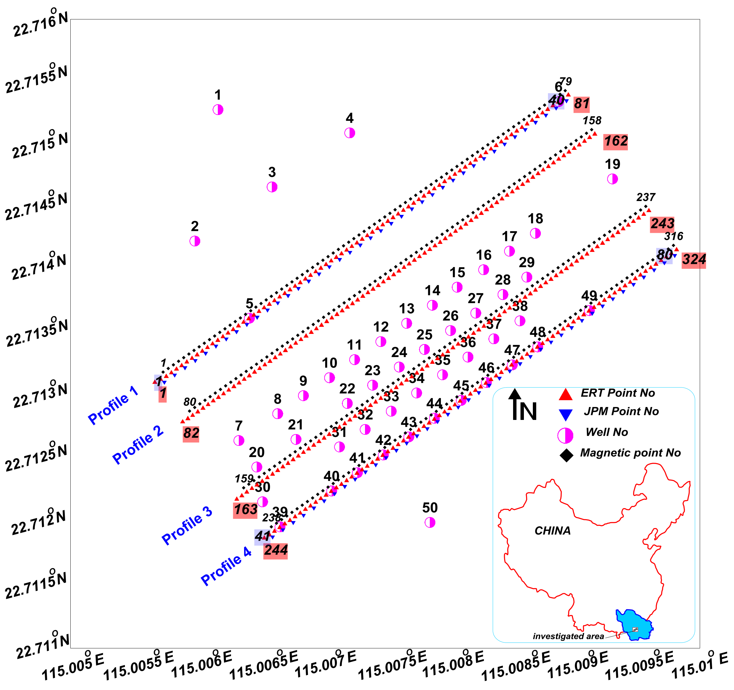
The simplified geological settings of the study area are given in the hydrogeological map as shown in Figure 2. Based on the geological settings, the investigated area is composed of volcanic and magmatic rocks/minerals of Jurassic age such as volcano dust, matrix, quartz, pyrite sulfide, feldspar, pyroxene, and basalts with some quartz veins embedded in the Aeolian tuff rock [41]. Various factors control the groundwater potential, occurrence and its flow in the study area such as hydrothermal processes, tectonic forces associated with weathering, fracturing, and fissuring, and secondary alteration of veins that contains high concentration of structural, lithological, and compositional heterogeneities that cause the water circulation [41]. The weathering processes play a major role to facilitate the water infiltration and its transportation in the top surface layer. Hydrogeologically, the weathering assists to make up the crucial period for the occurrence of groundwater reserves [42]. In the investigated area, the main aquifer is found in the upper layer formed by weathering, fissuring, and fracturing. Several boreholes were conducted in this investigation to reveal the existence of weathering, fissuring, and fracturing in the subsurface formation. Generally, the water level varies from 2 m to 32 m below the top surface, and from 106 m to 148 m with the elevation. In addition to above factors, various faults, the dynamo metamorphic zone and an unconformable boundary make the hydrogeological conditions more complex in the area to study the groundwater potential in hard rock aquifer (Figure 2). The topographic variations in the study area are shown in Figure 3. Electrical resistivity tomography (ERT) survey integrated by borehole, JPM and magnetic method was conducted in Huidong area by a joint project of University of Chinese Academy of Sciences, Institute of Geology and Geophysics to assess the subsurface hydrogeological conditions for groundwater potential. Figure 1 shows the location of the study area with the measurements of ERT, JPM, magnetic and borehole data.
3. Materials and Methods
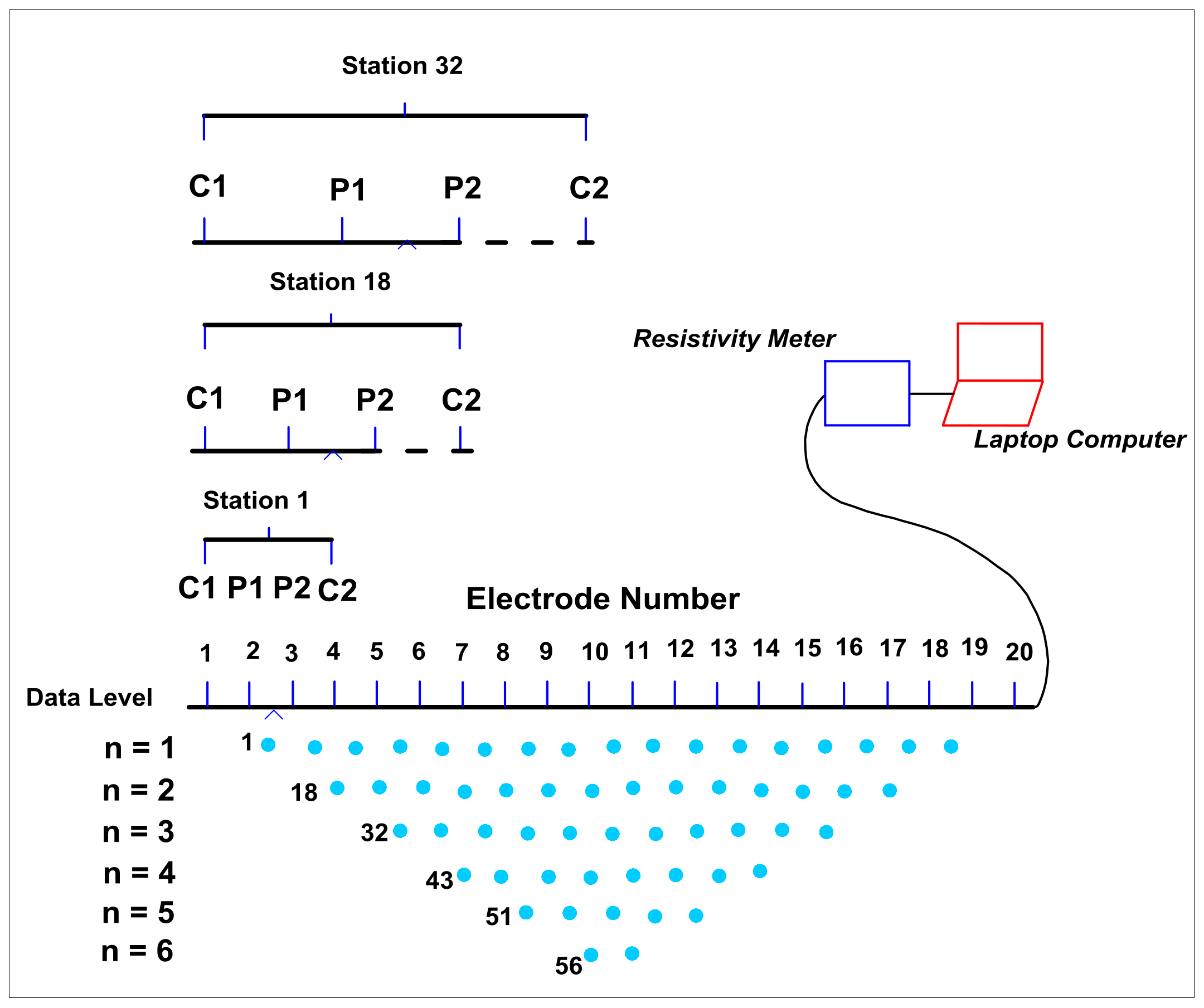
In this survey, ERT method with ABEM Lund Imaging System (Lund University, Lund, Sweden) [16] was applied using different layouts. This is an automated imaging system for the collection, processing, and presentation of resistivity. This method is based on the conductivity difference between the rock formation and the surrounding materials. By studying the underground steady electric field, this method is a very useful exploration tool to solve the engineering hydrogeological problems. The resistivity imaging is a recently developed modern technique to investigate the subsurface characteristics of the areas with complex geological settings where the applications of other methods such as resistivity soundings are not affective [43]. This method is defined by the density, the arrangement of electrodes and the amount of information to be acquired. ERT provides the subsurface geologic information through the corresponding interpretation using a software. An example for the principle of building up a resistivity pseudo-section using ABEM Terrameter with a system of 20 electrodes for pole-dipole array is given in Figure 4. It is a multi-function electrical instrument that has a multi-electrode convertor for the observations. Electrical resistivity tomography (ERT) is cost effective, fast, and versatile technique for mapping the groundwater conditions and assessing the shallow subsurface anomalies [44]. This technique is useful to obtain the important information for the planning of groundwater exploration. By increasing the electrode spacing, it can measure a series of constant separation traverses. Since increasing the separation provides more depth penetration, the vertical contoured image of measured apparent resistivity shows lateral and vertical variations in apparent resistivity over the section. The important geological units such as weathered/partly weathered/fissured layers, fractures and faults associated with the groundwater occurrence in the area were the main targets under this investigation. Different rock types (weathered rocks, partly weathered rocks, unweathered rocks), fractures, fissures, streams, or springs in the surroundings were considered as important aspects in selecting the locations for the resistivity lines. It was also very important to get the useful geological information in situ by drilling the boreholes. The slurry hole-boring method was used for drilling without using any metallic casing in this investigation.
Electrical resistivity tomography (ERT) is a complete automated technique that is employed using several electrodes joined by a multicore cable. The positions of current and potential electrodes are adjusted by a resistivity meter using a microprocessor controlled electronic module. Before starting the field measurements, a specific electrode configuration with fixed electrode spacing and all other required information is provided to the resistivity meter through a computer and resistivity data is collected automatically through this arrangement. To get the accurate position of the profiles and electrodes, surveying instrumentation and GPS systems (MAP60, Garmin, Olathe, KS, USA) were used in the field measurements. Commercially available software (prosys-geotomo software) is used to process this field data in different stages. The obtained apparent resistivity data is inverted by the software to generate a 2D image of the modeled resistivity along the profile. 2D as well as a 3D image of the subsurface can be obtained using the proper survey pattern and data procedure. In this study, 2D resistivity imaging was used along four profiles. Pole-dipole configuration was used to collect the resistivity data along four profiles with remote pole at a distance of 3 to 4 times the array length, and with each profile carrying a total of 81 electrodes, 5 m electrode spacing and a spread length of 400 m. The data acquisition was performed for 25 layers along each profile. The data were collected by applying a Terrameter SAS4000, ES10-64C switcher (Lund University, Lund, Sweden) and 12 V battery. The topography along the profiles was obtained with the measurements of every 10 m using a clinometer. The signal to noise ratio was improved using a single point data collected with maximum 10 stacking. During the processing of resistivity data, the bad quality data were filtered, and good quality data were used as input to RES2DINV software [3,12,45,46]. RES2DINV software (v3.50, Geotomo software Company, Penang, Malaysia) is an inverse program that is used to generate a 2D resistivity picture of the subsurface. RES2DINV is a least-squares inversion technique that must apply a smoothness constraint [47,48]. This inversion procedure generates a smooth model that can fit the data to a given level of error. In this survey, RMS error (difference in calculated and apparent resistivity values) for all inversion models was less than 5%. This model consists of several rectangular blocks equal to the data points of the resistivity pseudo-section. The central depth of the interior blocks is placed at the median depth of investigation [49]. The conventional Gauss-Newton least squares method [50] is an inversion scheme that can be used to minimize the difference between measured and modeled resistivity data. The smoothness-constrained modified model of Gauss-Newton [47] is based on the following equation:
where
(JiTJi + λiCTC)pi = JiTgi
- i = iteration number
- Ji = Jacobian matrix of partial derivatives
- gi = discrepancy vector
- λi = damping factor
- pi = perturbation vector to the model parameters for the ith iteration
- C = 2D flatness filter
where gi depends on the difference between the logarithms of the measured and calculated values of apparent resistivity, C is applied for constraining the smoothness of the perturbations for some constant value of the model parameters [51], and λ depends on the random noise of the data and its large value is used for high noise. The partial derivatives of a block are independent of the block size, which decrease with increasing distance to the electrodes. The amplitude of C for each row increases by 10% for stabilizing the inversion. CTC is sparse and symmetric. The first step in the least squares inversion is to calculate the apparent resistivity, the second step is to calculate Jacobian matrix J and the third step is to solve the above system of the linear equations. The finite difference or finite element methods can be used to complete the first two steps, whereas the third step can be solved using number of techniques such as the modified Gram-Schmidt, Cholesky and singular value decomposition methods [52].
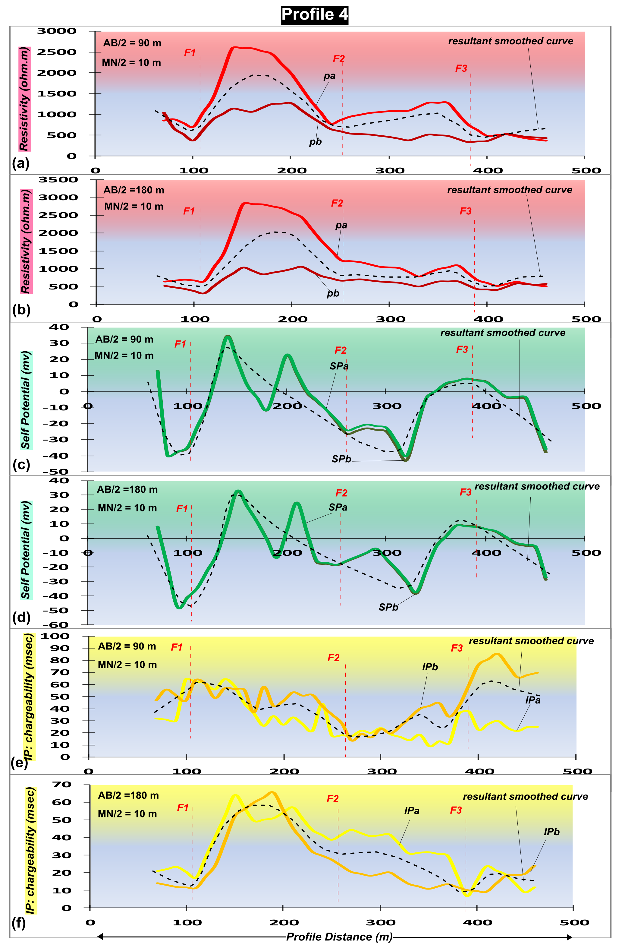
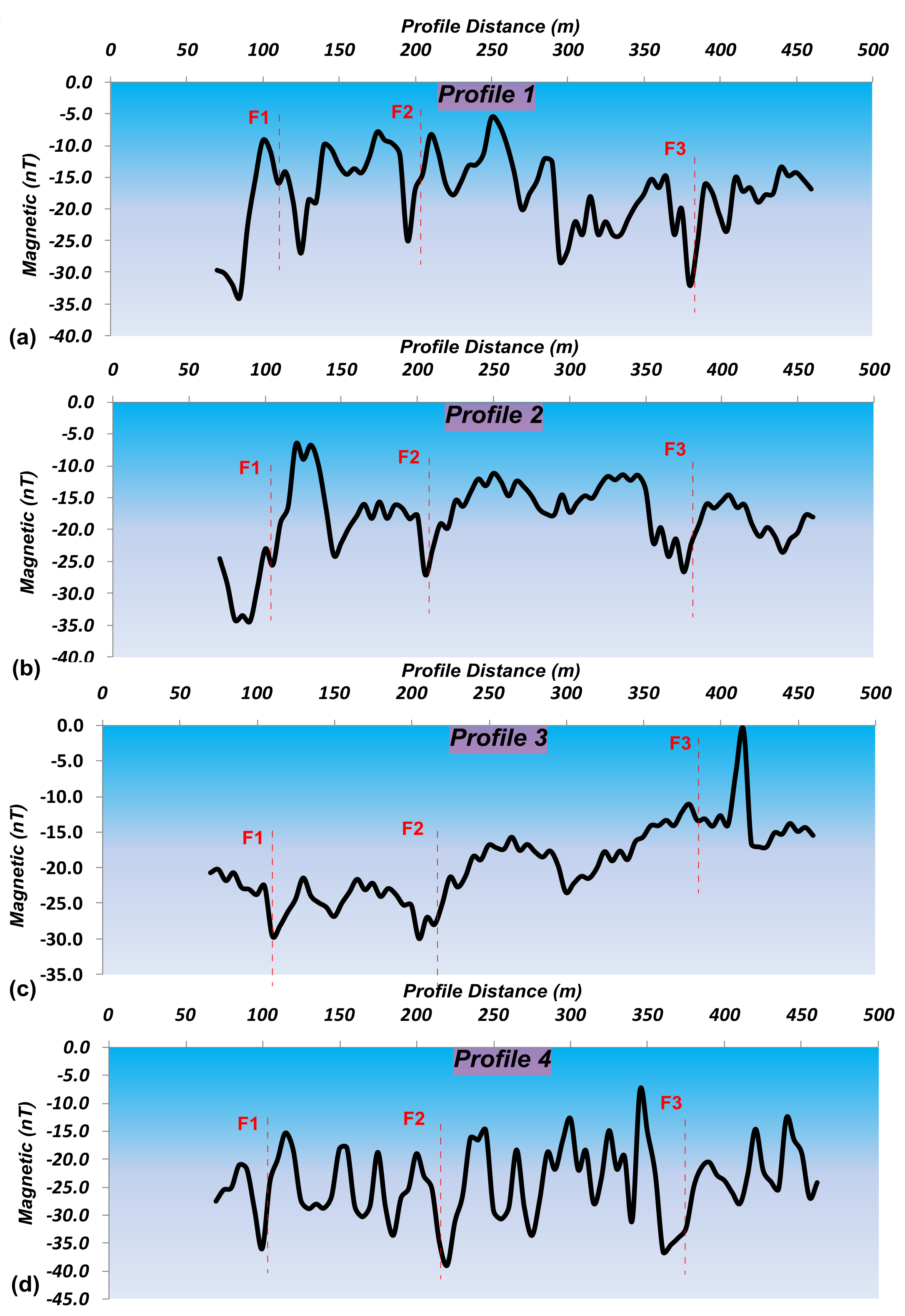
In this study, ERT provides the subsurface image up to 50 m depth. The depth of the investigation depends on the factors such as array type, number of electrodes, electrode spacing, number of segments and the ability of equipment to measure the signal (i.e., amplitudes of the signal and the noise, power specification of the equipment and its ability to filter the noise through stacking process). To calculate the maximum depth of the investigation, the maximum electrode spacing or the maximum array length was multiplied by the ratio of median depth of investigation to the electrode spacing or the total electrode spacing [11]. To delineate the main faults along all profiles, ERT sections were integrated with Joint Profile Method (JPM) and magnetic data. Joint Profile Method (JPM) was performed along two of the four profiles to observe the alterations in resistivity, self potential (SP) and induced polarization (IP) at 90 m and 180 m depth (AB/2 = 90 m, MN/2 = 10 m and AB/2 = 180 m, MN/2 = 10 m, where AB/2 is the depth and MN/2 is the electrode spacing). JPM provides composite joint curves for resistivity, SP, and IP at greater depths (90 m and 180 m). In this method, a multi-function electric instrument WDJD-4 (Chongqing Pentium Research Center, Chongqing, China) was used. The joint cross section device of JPM is shown in Figure 5. The joint curves of resistivity, SP, and IP show clear alterations along the main faults at greater depths which are consistent with the ERT sections. Magnetic data was plotted to observe the alterations in magnetic curves along the main faults, which shows consistency with ERT and JPM for the identification of main faults.
The topography and the lithostratigraphic information from the borehole data were integrated into the ERT profiles. After the data processing was completed, the results were interpreted for presentation by setting a resistivity range suitable for the expected hydrogeological features for each profile in the investigated area. A conceptual model of hydrogeological properties in the weathered environment of the study area was generated as shown in Figure 6. This model explains a complete concept for the groundwater occurrence in such complex weathered environment.
4. Results
Using the ERT method, the resistivity data were obtained and processed by RES2DINV software [3,12]. RES2DINV is a Windows-based computer program that is used to obtain a two-dimensional (2D) resistivity image of the subsurface. The processed data show the modeled resistivity sections with the topography along four profiles with the color infill. The data were inverted to obtain the ERT sections. After the correlation of resistivity images with the borehole lithology, ERT sections were interpreted into three layers with different resistivity ranges as shown in Table 1. The first distinct layer in the model is highly weathered rock underlying the top surface with resistivity range of 22 Ωm–345 Ωm and an average thickness of 20 m. Partly weathered rock is the second layer revealed underneath the top layer with an average thickness of 10 m and resistivity ranging from 324 Ωm to 926 Ωm. The fresh basement is the third layer encountered at an average depth of 20 m, its resistivity values range from 913 Ωm to 2579 Ωm. Table 1 shows the main distinct layers revealed in the study area with different resistivity ranges based on the calibration of resulted ERT sections with the borehole data. Since the resistivity of the materials is inversely proportional to the percent water saturation, the low resistive materials clearly show the water saturation. Furthermore, clay can also have a significant effect on resistivity values. Resistivity decreases with the increase of clay content. Borehole data revealed 2 m–5 m thick topsoil layer with silt/clay content in the study area. Figure 7 shows the position of the water table in the study area. Generally, the water level in the study area lies within the weathered rock; it varies from 2 m to 32 m with respect to the depth and from 106 m to 148 m with respect to the elevation. The modeled ERT sections and supplemented SP and IP measurements are shown in Figure 8, Figure 9, Figure 10, Figure 11, Figure 12 and Figure 13. The modeled ERT sections are shown in Figure 8 and Figure 10, Figure 11 and Figure 12. Three main faults (F1, F2 and F3) were identified by the integration of ERT sections with JPM and magnetic data. The delineation of the faults and weathered layers is very important because the groundwater reserves are contained in the weathered/fault zones. The magnetic susceptibility of weathered/fractured or fault zones is low, whereas it is high for unweathered/fresh basement rock. Therefore, this significant susceptibility contrast between weathered/fault zone and unweathered zone reveals a useful information for the groundwater occurrence in weathered/fault zone. SP and IP measurements were used to supplement the ERT results for the delineation of main faults which contain the groundwater reserves. SP is sensitive to the groundwater flow and its negative values suggest the groundwater saturated fractured/fault zone. IP identifies the electrical chargeability of the subsurface materials. A careful observation shows that faults zones containing the groundwater reserves in the study area are characterized by low values of resistivity, SP and IP as shown in Figure 9 and Figure 13.
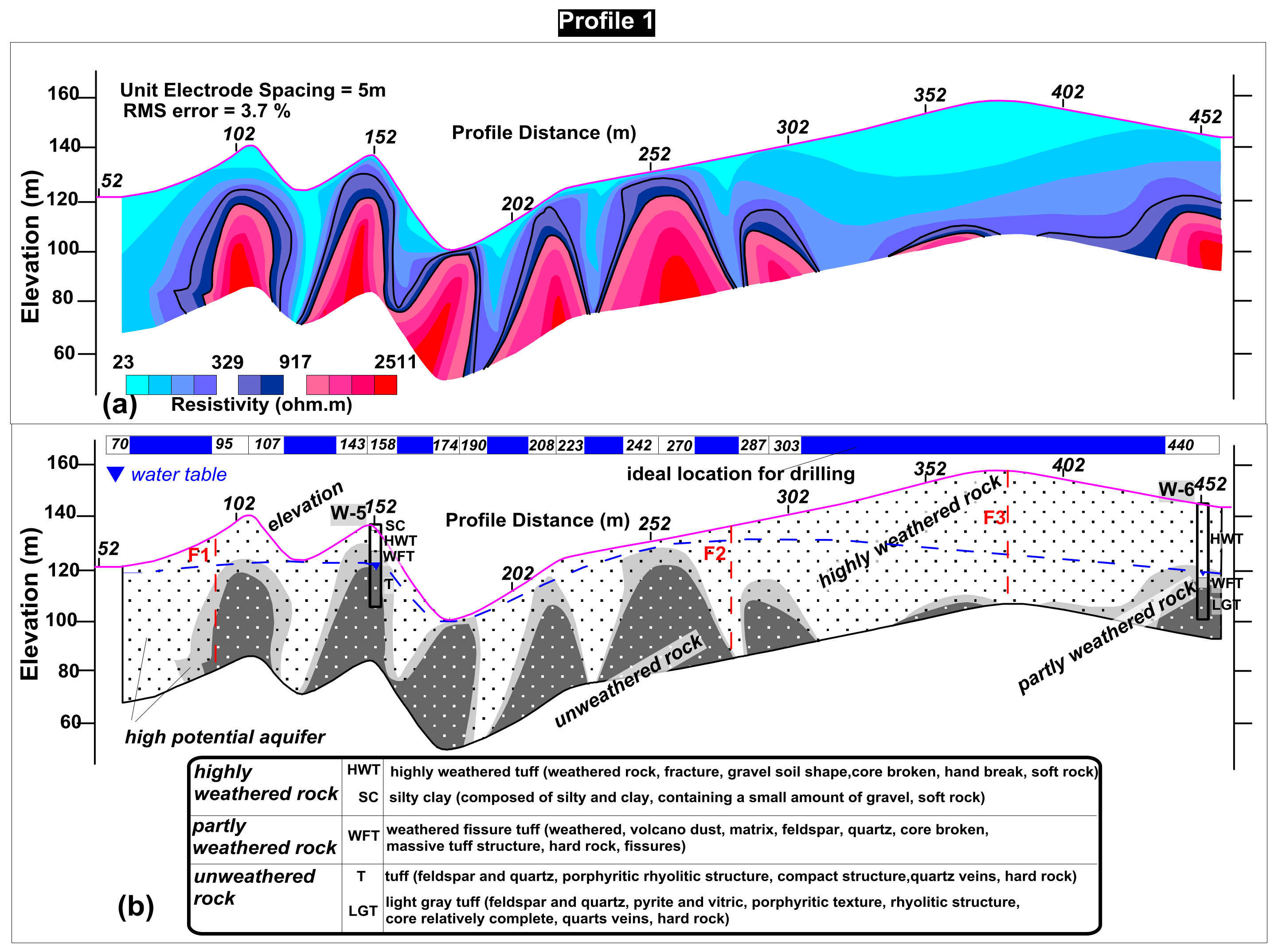
4.1. Profile 1
The imaging method encountered three distinct layers namely highly weathered rock, partly weathered rock, and the fresh bedrock along the profile 1 as shown in Figure 8. The top distinct layer is highly weathered layer with an average thickness of 20 m, and it contains weathered tuff rock, silt and clay and other weathered materials with resistivity ranging from 23 Ωm to 329 Ωm. The top layer extends to the partly weathered layer which is 10 m thick and its resistivity ranges from 329 Ωm to 917 Ωm mainly composed of weathered fissure tuff rock with volcano dust, matrix, feldspar, quartz etc. Fresh basement rock is encountered under the partly weathered layer at an average depth of 20 m with resistivity values ranging from 917 Ωm to 2511 Ωm. The bedrock contains unweathered tuff rock mainly consisted of feldspar, quartz, pyrite etc. Groundwater in the Basement Complex is generally found in the weathered, fractured, fissured, and jointed systems of the bedrock [55]. The low resistive layers indicate the presence of water. Highly weathered and partly weathered layers are the most promising water-bearing layers in the study area. Figure 8 shows the interpreted resistivity section of three distinct layers with the borehole information along profile 1. Three main faults (F1, F2 and F3) were identified along this profile in northeast to southwest (South China Sea) direction. The suitable locations for drilling were marked by the horizontal thick blue line as shown in Figure 8b. The conditioning of groundwater is the thickness of the aquifer layer and Figure 8 shows good locations to drill a borehole, for instance at 70 m to 95 m, 107 m to 143 m, 158 m to 174 m, 190 m to 208 m, 223 m to 242 m, 270 m to 287 m and 303 m to 440 m.
Using JPM, the resistivity, SP and IP composite joint curves were plotted at 90 m and 180 m depths to observe the alterations in the curves along the main faults as shown in Figure 9. Magnetic data was also plotted to see the variations in magnetic values along the identified faults (Figure 14a). The resistivity, SP, IP, and magnetic curves show clear alterations along the main faults integrated by ERT.
4.2. Profile 2
No borehole was drilled along this profile 2 (Figure 10). Based on nearby borehole data, three layers were identified (Figure 10). The first prominent layer under the top surface is highly weathered rock mainly consisting of volcanic tuff rock and other weathered materials with resistivity range of 27 Ωm–334 Ωm and an average thickness of 20 m. The partly weathered bedrock is the next layer underlying the top layer with an average thickness of 10 m and resistivity ranging from 334 Ωm to 921 Ωm. This layer is composed of weathered fissured tuff rock with volcano dust, matrix, feldspar, quartz etc. Highly weathered and partly weathered layers are the best for groundwater occurrence along this profile. The fresh bedrock is the third layer identified at an average depth of 20 m with resistivity value as low as 921 Ωm and as high as 2579 Ωm mainly composed of unweathered tuff with feldspar, quartz, pyrite etc. This layer is not ideal for aquifer occurrence, but it may be used as pillar support for buildings or other engineering structures. The expected water level position along this profile is also shown in Figure 10. Three main faults (F1, F2 and F3) were revealed by ERT and magnetic data (Figure 14b) along profile 2 in the orientation of northeast to southwest. The ideal location for drilling along this profile was marked from 70 m to 100 m, 135 m to 155 m, 185 m to 230 m and 350 m to 450 m (Figure 10b).
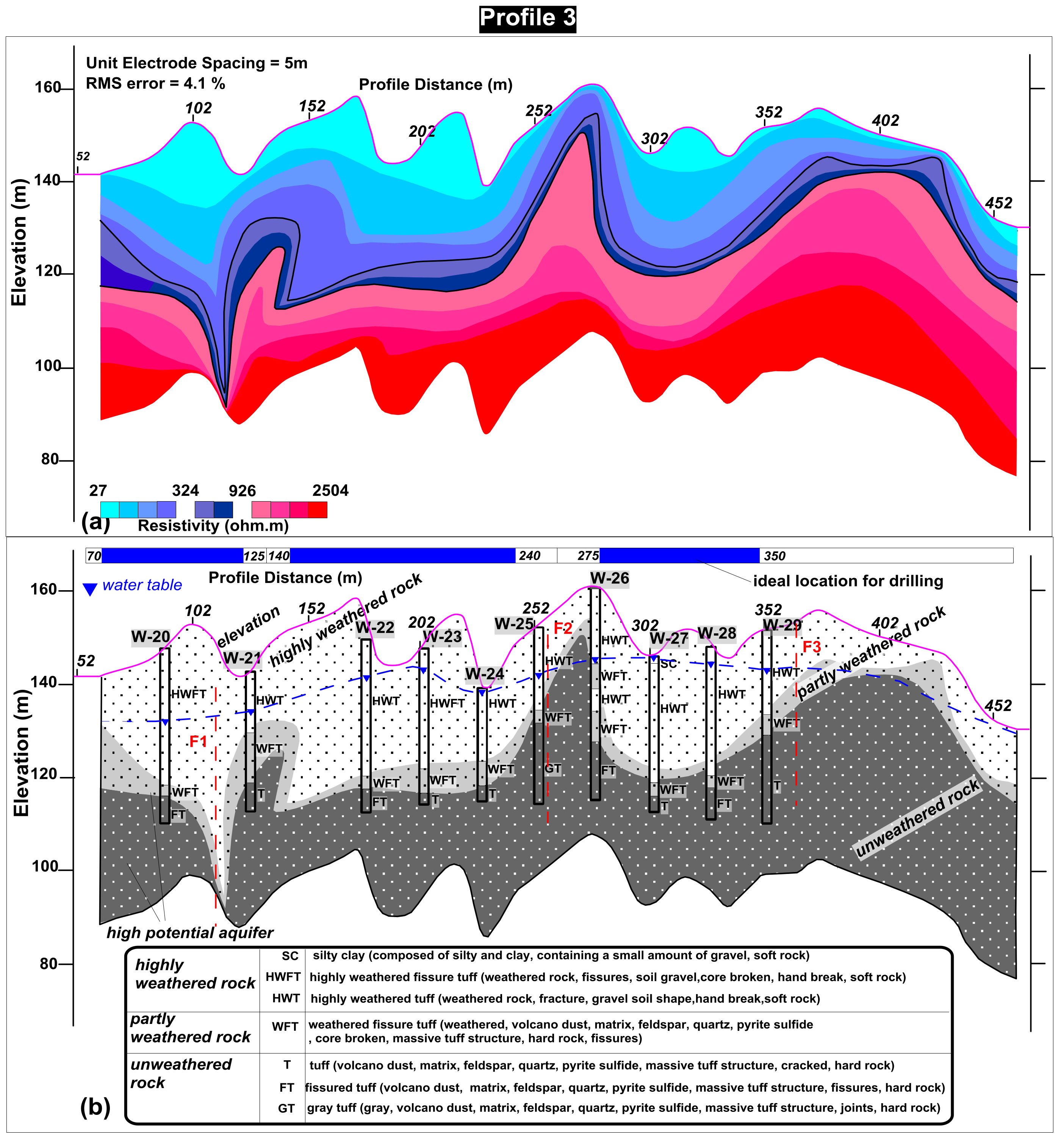
4.3. Profile 3
Ten boreholes were drilled along profile 3. This profile shows an electrical section of three layers depending on the integrated results of ERT and the borehole data (Figure 11). The first distinct layer exposed under the top surface is highly weathered, which has an average thickness of 20 m with resistivity range of 27 Ωm–324 Ωm mainly containing weathered tuff and weathered fissure tuff with silt and clay and other weathered materials. Underlying the top layer, a partly weathered layer is revealed with resistivity ranging from 324 Ωm to 926 Ωm and an average thickness of 10 m. It consists of weathered fissure tuff with volcano dust, matrix, feldspar, quartz, and pyrite sulfide. These two layers are ideal location to drill the boreholes for groundwater exploration. At an average depth of 20 m, unweathered layer is encountered which is the fresh basement rock with resistivity range of 926 Ωm–2504 Ωm, it is mainly composed of tuff, fissured tuff and gray tuff containing volcano dust, matrix, feldspar, quartz, pyrite sulfide etc. This layer is good for engineering structures rather than aquifer potential. Figure 11 shows the position of water table which mostly lies within the weathered layer. Three faults identified along first two profiles also extend to this profile with the same orientation. The main faults (F1, F2 and F3) were delineated by the integration of ERT with magnetic data (Figure 14c). The most suitable drilling locations along this profile were found at the distance from 70 m to 125 m, 140 m to 240 m and 275 m to 350 m (Figure 11b).
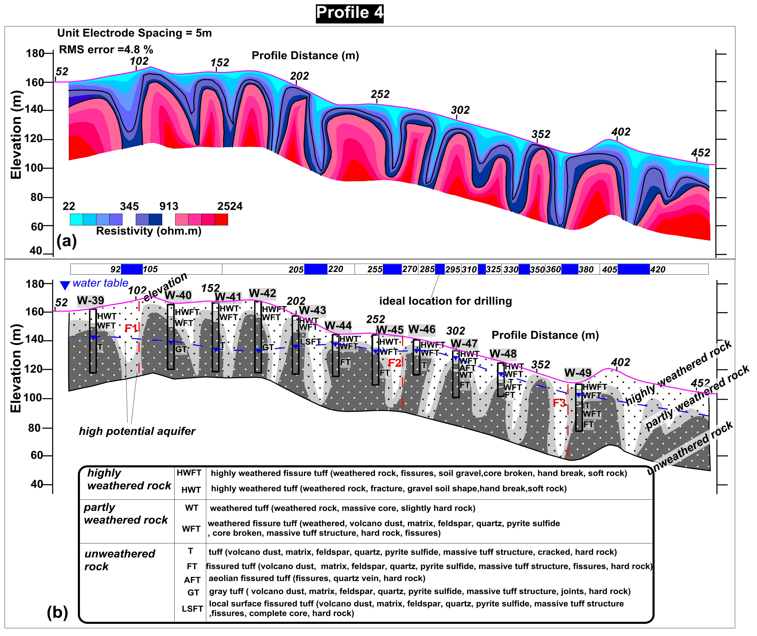
4.4. Profile 4
This profile reveals three distinct layers namely highly weathered, partly weathered, and unweathered layer, based on the lithology of eleven borehole data (Figure 12). The first layer on ERT section of this profile is highly weathered mainly composed of weathered tuff, weathered fissure tuff and other weathered materials with an average thickness of 20 m and resistivity range of 22 Ω m–345 Ωm. Partly weathered layer is the next layer with resistivity ranging from 345 Ωm to 913 Ωm and an average thickness of 10 m mainly consisting of weathered tuff and weathered fissure tuff and other rocks/minerals such as volcano dust, matrix, feldspar, quartz, pyrite sulfide etc. On reaching the average depth of 20 m, bed rock is encountered which is unweathered fresh basement with resistivity ranging from 913 Ωm to 2524 Ωm mainly composed of fresh tuff, fissured tuff, Aeolian fissured tuff, gray tuff, local surface fissured tuff with the rocks/minerals such as volcano dust, matrix, feldspar, quartz, pyrite sulfide etc. Highly weathered and partly weathered layers are the most promising water-bearing rocks along this profile. Three main faults (F1, F2 and F3) were also revealed along this profile at the same location in northeast-southwest direction (Figure 12b). The appropriate drilling locations along this profile can be found from 90 m to 105 m, 205 m to 220 m, 255 m to 270 m, 285 m to 295 m, 310 m to 325 m, 330 m to 350 m, 360 m to 380 m and 405 m to 420 m as shown in Figure 12b.
4.5. Analysis of Rock Samples
The X-ray Diffraction Technique (XRD) (D/Max-2400, Rigaku, Tokyo, Japan) was carried out for the mineral analysis of six rock samples collected from different places in the study area as shown in Figure 15. Four rock samples (1, 2, 3 and 4) from the weathered rock and two samples (5 and 6) from the bed rock were collected (Table 2). The XRD test was performed in X-ray Diffraction Analysis Laboratory of Institute of Geology and Geophysics, Chimes Academy of Sciences. Before the test, rock samples were grinded in the laboratory with the maximum particle size not more than 0.05 mm. The mineral analysis was performed using the instrument namely D/Max-2400 XRD ray diffractometer with the experiment conditions set as 40 kV and 60 mA with Cu target. The interpreted minerals were characterized as major (>50%), secondary (10–30%) and minor (5–10%). The results summarized in Table 2 show quartz as the major mineral; microcline, kaolinte, albite and zinnwaldite as the secondary minerals; and halloysite, perlite sodalite and akerite as the minor minerals in the investigated area. According to the XRD results, it can be found that samples 1 and 2 contain quartz up to 90% whereas other four samples contain quartz > 50% suggesting that quartz is the dominant mineral in the study area. The bedrock in the site area should be medium-acidic rock. The weathered rocks contain a certain amount of clay minerals such as kaolinite, halloysite, microcline and perlite especially the residual soil (sample 4) contains 10% to 30% kaolinite. The XRD results show that the residual kaolinite is mainly due to the weathering and conversion of feldspar, which often occurs in mountain basins and reflects the warm and humid climate. Fault sample (sample 3) contains pearlite (kaolinite), also known as pearl clay, which is related to the action of low-temperature hydrothermal fluids and reflects the tectonic movement of the faults. The bedrock samples contain the minerals such as quartz (>50%), albite and zinnwaldite (10–30%), and sodalite and akerite (5–10%).
4.6. Analysis of Water Samples
Water samples were collected from six different places in the investigated area as shown in Figure 15. Two (sample No. 1 and 2) of these six samples were collected from the fissure water (from bore-wells at an average depth of 40 m to 50 m) and other four samples (sample No. 3, 4, 5 and 6) were taken from the water channels. Water samples were collected using 500 mL plastic bottles of mineral water at noon. After the bottles were filled with water, bottle caps were tightened and sealed to avoid contamination. Before sample collection, the bottles were rinsed three to five times with water filtered through 0.5 mm mixed cellulose ester membrane. The samples were preserved at approximately 4 °C before the analysis. The water samples were analyzed as per standard procedure [56,57,58] for physicochemical parameters such as sodium (Na+),potassium (K+), calcium (Ca2+), magnesium (Mg2+), bicarbonate (HCO3−), chloride (Cl−), sulfate (SO42−), ammonium (NH4+), nitrate (NO3−), pH, electrical conductivity (EC) and total dissolved solids (TDS) in the Guangdong Geological Experimental Testing Center. The international standard referential materials and the synthetic solutions were applied to the samples in order to verify the accuracy. The physicochemical parameters were calculated using mean values. For the standard referential materials, recovery was found greater than 95%. To check the data quality, the charge balance for each water sample was determined and charge balance error for each analysis was found to be <±5% which is acceptable as shown in Table 3. The major element compositions of the samples were all lower than the guideline values for drinking water of the World Health Organization (WHO). However, we are not able to comment on the suitability of the waters for drinking in the absence of data on trace elements, organic constituents or pathogens. The pH values of six water samples are more than 7, so all of them are alkaline. However, the pH values of two samples (fissure water) are above 7.5, which are more alkaline than other four samples. pH values of four samples (water channels) are low probably due to the faster water channels flow and greater contact area with air than the fissure water, dissolving more CO2.
5. Discussion
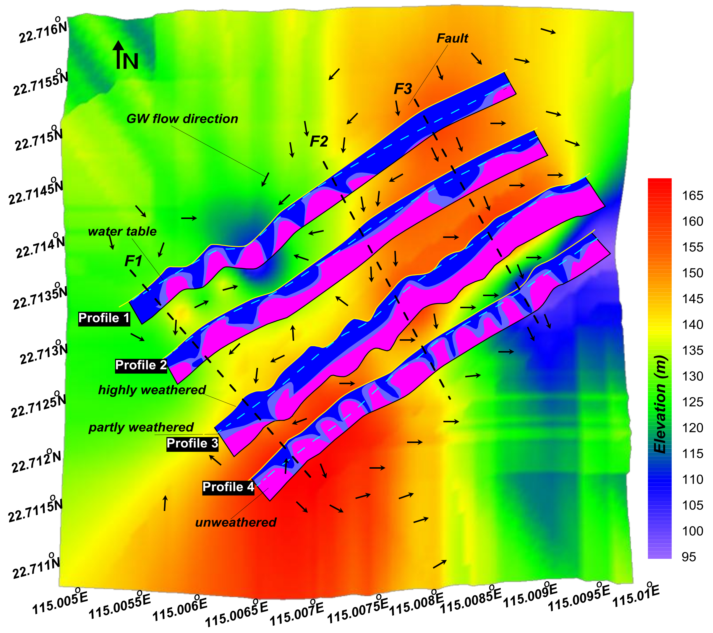
In this investigation, ERT method in combination with JPM, magnetic and borehole data was used to assess the groundwater potential in the hard rock aquifers of complex geological settings. Four profiles were interpreted using ERT to map the subsurface weathered/unweathered layers for groundwater occurrence. Most heterogeneous profiles 1 and 4 were interpreted by the integration of ERT with JPM and magnetic data for the delineation of main faults in the study area. The interpretation shows that the study area has complex geological environment with weathered, fractured, fissured, and faulted zones. The integrated results reveal that the top thick layer is highly weathered overlying the partly weathered/fissured layer. These two layers (highly weathered and partly weathered) are highly promising water-bearing strata in the investigated area. Three main faults (F1, F2 and F3) were delineated along four profiles showing northeast–southwest orientation. The identified faults show good consistency along all profiles. It was found that highly weathered, partly weathered and fault zones contain high potential groundwater reserves in the investigated area. A graphical representation of the measured parameters (topography, water table, weathered-partly weathered curve, unweathered-partly weathered curve, and main faults) is shown in Figure 16. Water table was measured two times, i.e., in December 2016 and September 2017. An increment in the water table was observed in September 2017 during the monsoon rainy season. Figure 17 shows the subsurface layers (highly weathered, partly weathered, and unweathered layers interpreted by ERT), the main faults (F1, F2 and F3 revealed by the integration of ERT with JPM and magnetic method), the topographic variations and the groundwater flow direction. In this study, ERT method was used to map the subsurface layers (highly weathered, partly weathered, and unweathered layer) in particular. ERT sections show various discontinuities along different profiles, since ERT provides subsurface information up to 50 m depth so it is not easy to identify the deep buried faults existing along all profiles. To identify the main faults extending from profile 1 to profile 4, ERT was integrated with Joint Profile Method (JPM) and magnetic method. JPM gives joint curves of resistivity, SP, and IP at greater depth of 90 and 180 m. The alterations in the curves of resistivity, SP, IP and magnetic were carefully observed and integrated with ERT to delineate the main faults (F1, F2 and F3). The identified faults extend from profile 1 to profile 4 in northeast-southwest direction, and are confirmed by the different methods (ERT, JPM and magnetic method). The interpreted faults also show good consistency along all profiles. The results of XRD technique shows that quartz is the major mineral, whereas microcline, kaolinite, albite, zinnwaldite are the secondary minerals; and halloysite, kaolinite, perlite, sodalite and ankerite are the minor minerals. The results of physicochemical analysis reveal that the water samples lie within the limit suggested by WHO.
6. Conclusions
In the ERT imaging method, four profiles were performed along the ground surface. The electrical imaging is more successful technique when it is compared with other geophysical methods to get a more detailed view of the subsurface features for better understanding of the groundwater occurrence in the weathered conditions. ERT is an inversion technique which can map the subsurface conditions even in the complex geological settings. This imaging method was performed using pole-dipole configuration and RES2DINV software to investigate the groundwater conditions in weathered environment of complex geology in the study area. The results revealed three distinct layers along four profiles in the study area based on the correlation of ERT resistivity images with the borehole data. The first distinct layer underlying the top surface is highly weathered layer mainly composed of weathered tuff, weathered fissure tuff, silt and clay and other weathered materials with an average thickness of 20 m and resistivity range of 22Ω m–345 Ωm. The second prominent layer is partly weathered underneath the top weathered layer with resistivity range of 324 Ωm–926 Ωm and an average thickness of 10 m mainly consisting of weathered tuff, weathered fissure tuff and other rocks/minerals such as volcano dust, matrix, feldspar, quartz, pyrite sulfide etc. These two layers are highly promising water-bearing strata in the study area. Generally, the groundwater reserves are contained within these two layers. The next layer underlying the partly weathered layer is unweathered which is fresh basement rock found at an average depth of 20 m with resistivity ranging from 913 Ωm to 2579 Ωm mainly composed of fresh tuff, fissured tuff with the rocks/minerals such as volcano dust, matrix, feldspar, quartz, pyrite sulfide etc. The integration of ERT with JPM and magnetic data reveals three main faults in the study area, which are consistent along all profiles. The weathered/partly weathered layers with low resistivity values clearly indicate the groundwater occurrence in the study area because the resistivity of rock decreases with the increasing of percent water saturation. The results reveal that weathered/partly weathered and faults zones are the best water-bearing strata for the groundwater potential in the investigated area.
Acknowledgments
This research was sponsored by CAS-TWAS (Chinese Academy of Sciences and The World Academy of Sciences) President’s Fellowship for International PhD Students; and funded by National Natural Science Foundation of China (Grant Nos. 41372324, 41772320), and Xinjiang Uygur Autonomous Region International Science and Technology Cooperation Program. Authors wish to acknowledge support received from Key Laboratory of Shale Gas and Geoengineering, Institute of Geology and Geophysics, Chinese Academy of Sciences, Beijing China.
Author Contributions
Qiang Gao and Muhammad Hasan conceived and designed the experiments; Peng Yang performed the experiments; Yanjun Shang analyzed the data; Qiang Gao and Muhammad Hasan wrote the paper.
Conflicts of Interest
The authors declare no conflict of interest.
References
- Dahlin, T. The development of electrical imaging techniques. Comput. Geosci. 2001, 27, 1019–1029. [Google Scholar] [CrossRef]
- Pellerin, L. Applications of electrical and electromagnetic methods for environmental and geotechnical investigations. Surv. Geophys. 2002, 23, 101–132. [Google Scholar] [CrossRef]
- Loke, M.H.; Barker, R.D. Rapid least-squares inversion of apparent resistivity pseudosections by a quasi-Newton method. Geophys. Prospect. 1996, 44, 131–152. [Google Scholar] [CrossRef]
- Loke, M.H.; Chambers, J.E.; Rucker, D.F.; Kuras, O.; Wilkinson, P.B. Recent developments in the direct-current geoelectrical imaging method. J. Appl. Geophys. 2013, 95, 135–156. [Google Scholar] [CrossRef]
- Binley, A.; Hubbard, S.S.; Huisman, J.A.; Revil, A.; Robinson, D.A.; Singha, K.; Slater, L.D. The emergence of hydrogeophysics for improved understanding of subsurface processes over multiple scales. Water Resour. Res. 2015, 51, 3837–3866. [Google Scholar] [CrossRef] [PubMed] [Green Version]
- Kemna, A.; Binley, A.; Ramirez, A.; Daily, W. Complex resistivity tomography for environmental applications. Chem. Eng. J. 2000, 77, 11–18. [Google Scholar] [CrossRef]
- Sandberg, S.K.; Slater, L.D.; Versteeg, R. An integrated geophysical investigation of the hydrogeology of an anisotropic unconfined aquifer. J. Hydrol. 2002, 267, 227–243. [Google Scholar] [CrossRef]
- Apparao, A.; Roy, A. Field results for direct current resistivity profiling with two-electrode array. Geoexploration 1973, 11, 21–44. [Google Scholar] [CrossRef]
- Verma, R.; Bandyopadhyay, T. Use of the resistivity methods in geological mapping-case histories from Raniganj Coalfield, India. Geophys. Prospect. 1983, 31, 490–507. [Google Scholar] [CrossRef]
- Batayneh, A.T. Resistivity imaging for near-surface resistive dyke using two-dimensional DC resistivity techniques. J. Appl. Geophys. 2001, 48, 25–32. [Google Scholar] [CrossRef]
- Loke, M.H. Tutorial: 2D and 3D Electrical Imaging Surveys; University of Alberta: Edmonton, AB, Canada, 2004; Available online: https://sites.ualberta.ca/~unsworth/UA-classes/223/loke_course_notes.pdf (accessed on 7 March 2018).
- Loke, M.H. Electrical Imaging Surveys for Environmental and Engineering Studies. A Practical Guide to 2D and 3D Surveys; Pergamon Press Inc.: Oxford, UK, 1966. [Google Scholar]
- Daniels, F.; Alberty, R.A. Physical Chemistry; John Wiley and Sons, Inc.: Hoboken, NJ, USA, 1966. [Google Scholar]
- Telford, W.M.; Geldart, L.P.; Sheriff, R.E. Applied Geophysics, 2nd ed.; Cambridge University Press: Cambridge, UK, 1990. [Google Scholar]
- Dahlin, T. 2D resistivity surveying for environmental and engineering applications. First Break 1996, 14, 275–283. [Google Scholar] [CrossRef]
- Seaton, W.J.; Burbey, T.J. Evaluation of two-dimensional resistivity methods in a fractured crystalline-rock terrain. J. Appl. Geophys. 2002, 51, 21–41. [Google Scholar] [CrossRef]
- Akhter, G.; Hasan, M. Determination of aquifer parameters using geoelectrical sounding and pumping test data in Khanewal District, Pakistan. Open Geosci. 2016, 8, 630–638. [Google Scholar] [CrossRef]
- Hasan, M.; Shang, Y.; Akhter, G.; Khan, M. Geophysical Investigation of Fresh-Saline Water Interface: A Case Study from South Punjab, Pakistan. Groundwater 2017, 55, 841–856. [Google Scholar] [CrossRef] [PubMed]
- Hasan, M.; Shang, Y.; Akhter, G.; Jin, W. Geophysical Assessment of Groundwater Potential: A Case Study from Mian Channu Area, Pakistan. Groundwater 2017. [Google Scholar] [CrossRef] [PubMed]
- Morse, M.; Lu, N.; Godt, J.; Revil, A.; Coe, J. Comparison of Soil Thickness in a Zero-Order Basin in the Oregon Coast Range Using a Soil Probe and Electrical Resistivity Tomography. J. Geotech. Geoenviron. Eng. 2012, 138, 1470–1482. [Google Scholar] [CrossRef]
- Palacky, G.J.; Kadekaru, K. Effect of tropical weathering on electrical and electromagnetic measurements. Geophysics 1979, 44, 69–88. [Google Scholar] [CrossRef]
- Doyle, H.A.; Lindeman, F.W. The effect of deep weathering on geophysical exploration in Australia—A review. Aust. J. Earth Sci. 1985, 32, 125–135. [Google Scholar] [CrossRef]
- Timms, W.; Acworth, I. Origin, lithology and weathering characteristics of Upper Tertiary—Quaternary clay aquitard units on the Lower Murrumbidgee alluvial fan. Aust. J. Earth Sci. 2002, 49, 525–537. [Google Scholar] [CrossRef]
- Kellett, R.; Bauman, P. Mapping groundwater in regolith and fractured bedrock using ground geophysics: A case study from Malawi, SE Africa. Recorder 2004, 29, 24–32. [Google Scholar]
- Barongo, J.O.; Palacky, G.J. Investigations of electrical properties of weathered layers in the Yala Area, Western Kenya, using resistivity soundings. Geophysics 1991, 56, 133–138. [Google Scholar] [CrossRef]
- Ritz, M.; Parisot, J.C.; Diouf, S.; Beauvais, A.; Dione, F.; Niang, M. Electrical imaging of lateritic weathering mantles over granitic and metamorphic basement of eastern Senegal, West Africa. J. Appl. Geophys. 1999, 41, 335–344. [Google Scholar] [CrossRef]
- Revil, A.; Hermitte, D.; Spangenberg, E.; Cochémé, J.J. Electrical properties of zeolitized volcaniclastic materials. J. Geophys. Res. 2002, 107, 2168. [Google Scholar] [CrossRef]
- Jardani, A.; Revil, A.; Barrash, W.A.; Crespy, E.; Rizzo, S.; Straface, M.; Cardiff, B.; Malama, C.; Miller, C.; Johnson, T. Reconstruction of the water table from self potential data: A Bayesian approach. Groundwater 2009, 47, 213–227. [Google Scholar] [CrossRef] [PubMed]
- Jardani, A.; Revil, A.; Santos, F.; Fauchard, C.; Dupont, J.P. Detection of preferential infiltration pathways in sinkholes using joint inversion of self-potential and EM-34 conductivity data. Geophys. Prospect. 2007, 55, 1–11. [Google Scholar] [CrossRef]
- Revil, A.; Murugesu, M.; Prasad, M.; Le Breton, M. Alteration of volcanic rocks: A new non-intrusive indicator based on induced polarization measurements. J. Volcanol. Geotherm. Res. 2017, 341, 351–362. [Google Scholar] [CrossRef]
- Johnson, T.C.; Versteeg, R.J.; Ward, A.F.; Day-Lewis, D.; Revil, A. Improved hydrogeophysical characterization and monitoring through high performance electrical geophysical modeling and inversion. Geophysics 2010, 75, WA27–WA41. [Google Scholar] [CrossRef]
- Schulz, R. Interpretation and depth of investigation of gradient measurements in direct current geoelectrics. Geophys. Prospect. 1985, 33, 1240–1253. [Google Scholar] [CrossRef]
- Shettigara, V.K.; Adams, W.M. Detection of lateral variations in geological structures using electrical-resistivity gradient profiling. Geophys. Prospect. 1989, 37, 293–310. [Google Scholar] [CrossRef]
- Furness, P. Gradient array profiles over thin resistive veins. Geophys. Prospect. 1993, 41, 113–130. [Google Scholar] [CrossRef]
- Kumar, D.; Anand, V.; Rao, V.A.; Sharma, V.S. Hydrogeological and geophysical study for deeper groundwater resource in quartzitic hard rock ridge region from 2D resistivity data. J. Earth Syst. Sci. 2014, 123, 531–543. [Google Scholar] [CrossRef]
- Szalai, S.; Novak, A.; Szarka, L. Which geoeletric array sees the deepest in a noisy environment? Depth of detectability values of multielectrode systems for various two dimensional models. Phys. Chem. Earth 2011, 36, 1398–1404. [Google Scholar] [CrossRef]
- Dahlin, T.; Zhou, B. A numerical comparison of 2D resistivity imaging with 10 electrode arrays. Geophys. Prospect. 2004, 52, 379–398. [Google Scholar] [CrossRef]
- Pous, J.; Queralt, P.; Chavez, R. Lateral and topographical effects in geoelectric soundings. J. Appl. Geophys. 1996, 35, 237–248. [Google Scholar] [CrossRef]
- Tsourlos, P.; Szymansky, J.; Tsokas, G. The effect of terrain topography on commonly used resistivity arrays. Geophysics 1999, 64, 1357–1363. [Google Scholar] [CrossRef]
- Bureau of Geology and Mineral Resources of Guangdong Province (Guangdong, B.G.M.R.). Regional Geology of Guangdong Province; Geology Publishing House: Beijing, China, 1988; pp. 1–602. (In Chinese)
- Mendoza, J.A. Geophysical and Hydrogeological Investigations in the Rio Sucio Watershed, Nicaragua; Lund University: Lund, Sweden, 2002; ISBN 919724060X. [Google Scholar]
- Griffiths, D.H.; Barker, R.D. Two-dimensional resistivity imaging and modeling in areas of complex geology. J. Appl. Geophys. 1993, 29, 211–226. [Google Scholar] [CrossRef]
- Kumar, D. Efficacy of electrical resistivity tomography technique in mapping shallow subsurface anomaly. J. Geol. Soc. India 2012, 80, 304–307. [Google Scholar] [CrossRef]
- Loke, M.H.; Barker, R.D. Leastsquares deconvolution of apparent resistivity pseudosections. Geophysics 1995, 60, 1682–1690. [Google Scholar] [CrossRef]
- Loke, M.H. RES2DINV Software User’s Manual, Version 3.57; Geotomo Software: Penang, Malysia, 2007; p. 86. [Google Scholar]
- De Groot-Hedlin, C.; Constable, S.C. Occam’s inversion to generate smooth, two-dimensional models from magnetotelluric data. Geophysics 1990, 55, 1613–1624. [Google Scholar] [CrossRef]
- Ellis, R.G.; Oldenburg, D.W. Applied geophysical inversion. Geophys. J. Int. 1994, 116, 5–11. [Google Scholar] [CrossRef]
- Edwards, L.S. A modified pseudosection for resistivity and induced-polarization. Geophysics 1977, 42, 1020–1036. [Google Scholar] [CrossRef]
- Lines, L.R.; Treitel, S. Tutorial: A review of the least-squares inversion and its application to geophysical problems. Geophys. Prospect. 1984, 32, 159–186. [Google Scholar] [CrossRef]
- Sasaki, Y. Resolution of the resistivity tomography inferred from numerical simulation. Geophys. Prospect. 1992, 40, 453–464. [Google Scholar] [CrossRef]
- Golub, G.H.; Van Loan, C.F. Matrix Computations; Johns Hopkins University Press: Baltimore, MD, USA, 1989. [Google Scholar]
- American Board of Emergency Medicine (ABEM). Terrameter SAS4000/SAS1000 LUND Imaging System, Instruction Manual; ABEM Instrument AB: Sundbyberg, Sweden, 2006. [Google Scholar]
- Wyns, R.; Gourry, J.C.; Baltassat, J.M.; Lebert, F. Multiparameter characterization of subsurface horizons (0–100 m) in an altered basement context. In Proceedings of the 2nd GEOFCAN Symposium, Orleans, France, 21–22 September 1999; pp. 105–110. [Google Scholar]
- Jones, M.J. The Weathered Zones Aquifers o Basement Complex Area of African. Q. J. Eng. Geol. Lond. 1985, 18, 35–45. [Google Scholar] [CrossRef]
- American Public Health Association (APHA); American Water Works Association (AWWA); Water Environment Federation (WEF). Standard Methods for theExaminations of Water and Wastewaters, 19th ed.; American Public Health Association: Washington, DC, USA, 1995; Volume 4. [Google Scholar]
- Radojevic, M.; Bashkin, V.N. Practical Environmental Analysis; Royal Society of Chemistry: Cambridge, UK, 1999. [Google Scholar]
- Hasan, M.; Shang, Y.; Akhter, G.; Jin, W. Evaluation of Groundwater Suitability for Drinking and Irrigation Purposes in Toba Tek SinghDistrict, Pakistan. Irrig. Drain. Syst. Eng. 2017, 6, 185. [Google Scholar] [CrossRef]
- World Health Organization (WHO). Recommendations Incorporating 1st and 2nd Addenda. In Guidelines for Drinking-Water Quality, 3rd ed.; World Health Organization: Geneva, Switzerland, 2008; Volume 1. [Google Scholar]
Figure 1.
Location map of the study area.

Figure 2.
Hydrogeological map of the study area (modified after [41]).
Figure 2.
Hydrogeological map of the study area (modified after [41]).
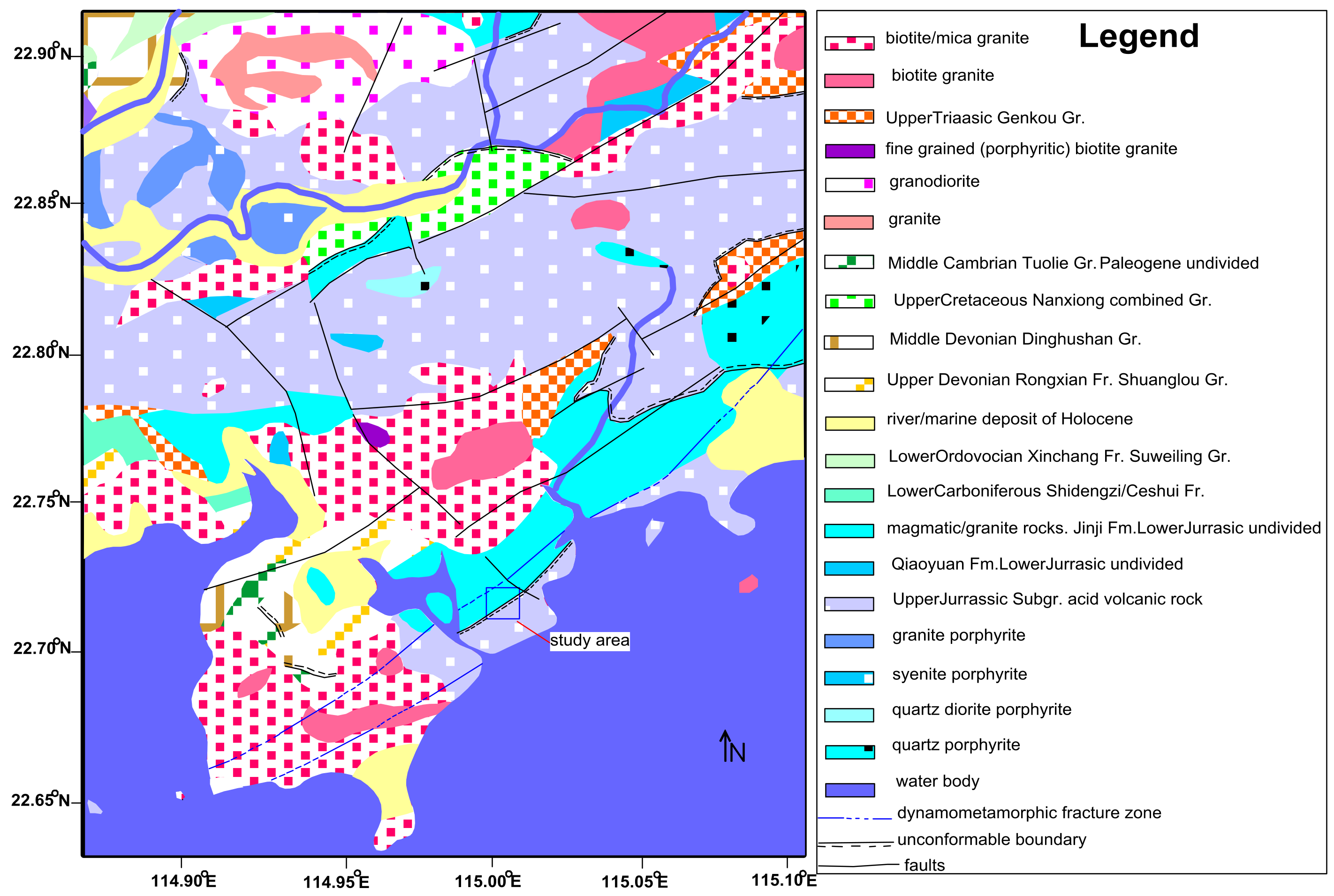
Figure 3.
Topography map of the study area.
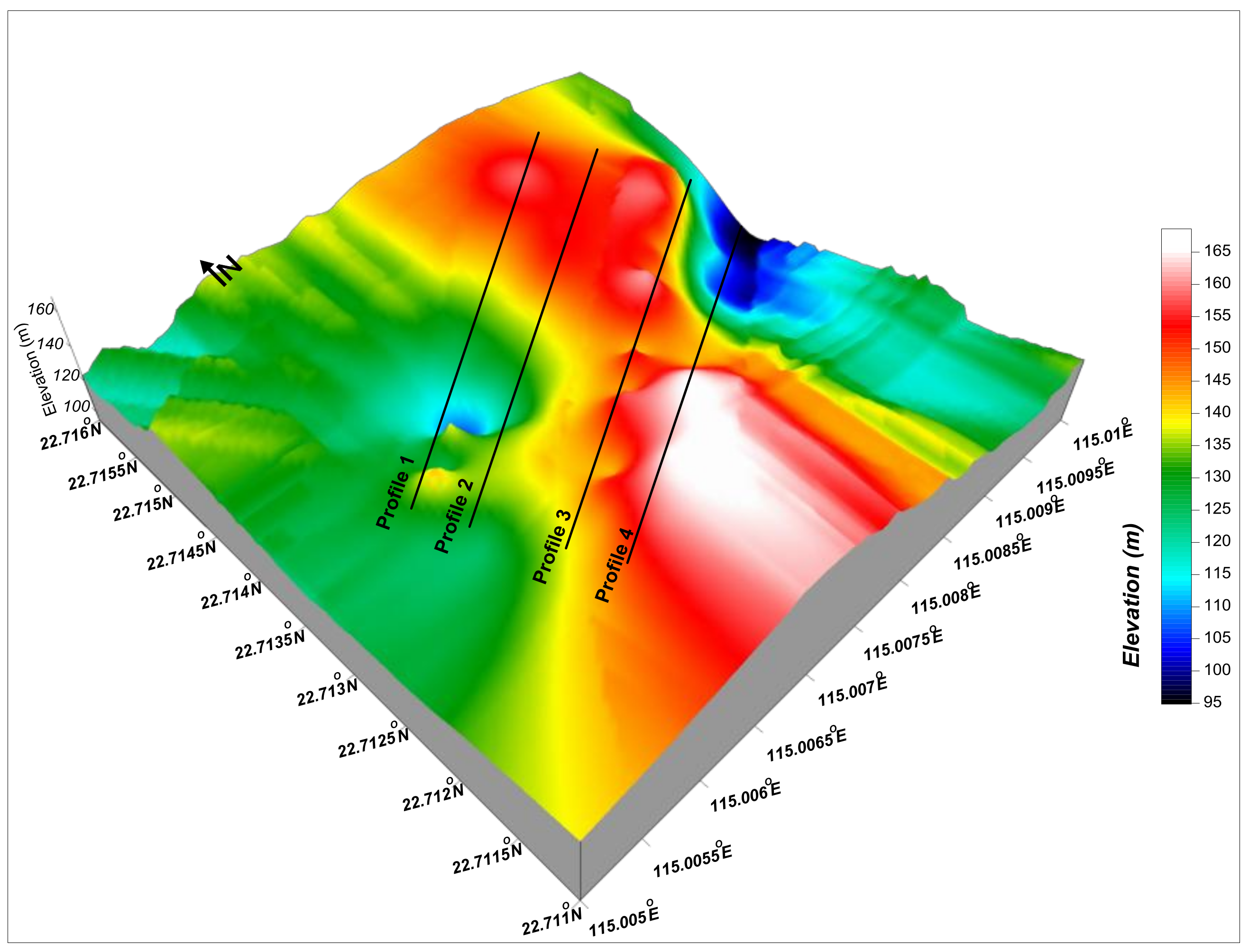
Figure 4.
Principle for building up a pseudo-section using pole-dipole array (modified after [53]).
Figure 4.
Principle for building up a pseudo-section using pole-dipole array (modified after [53]).

Figure 5.
Joint cross-sectional view of the device.
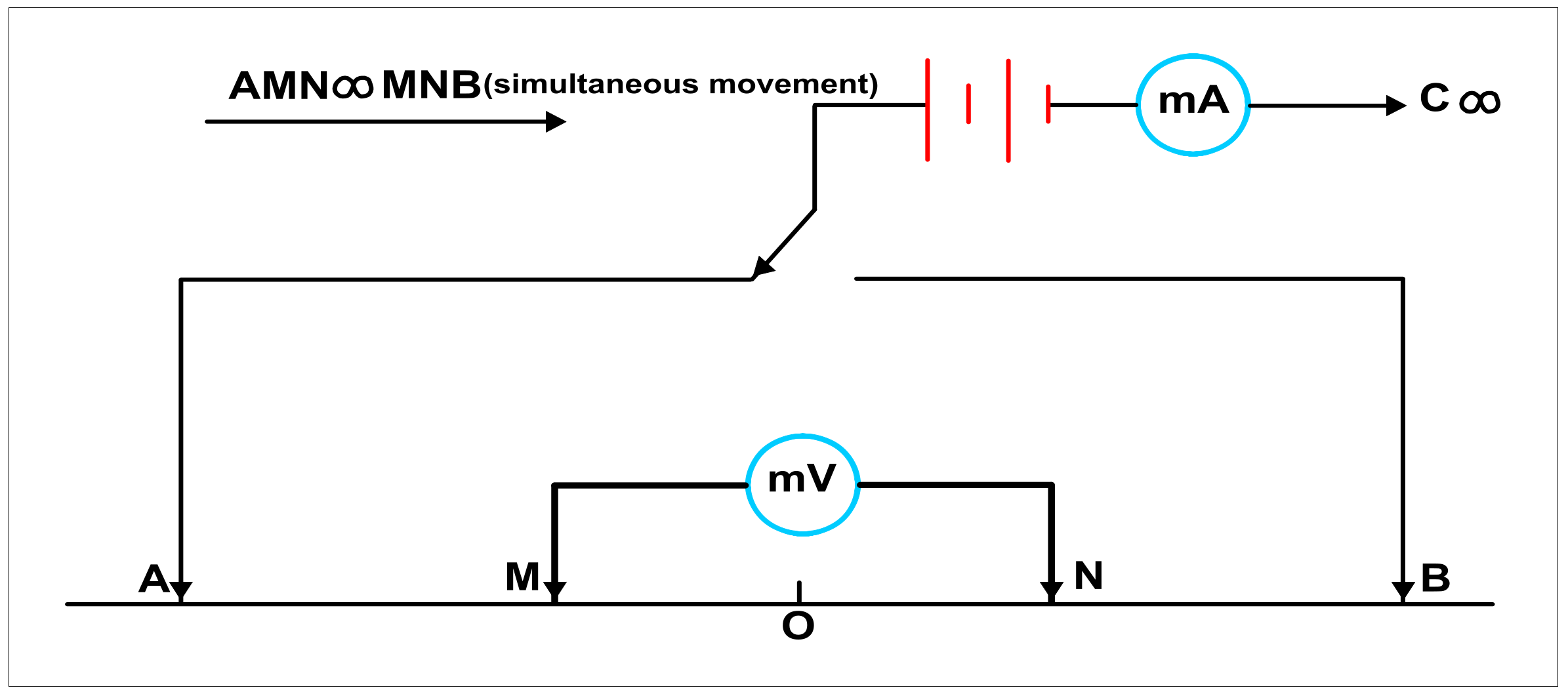
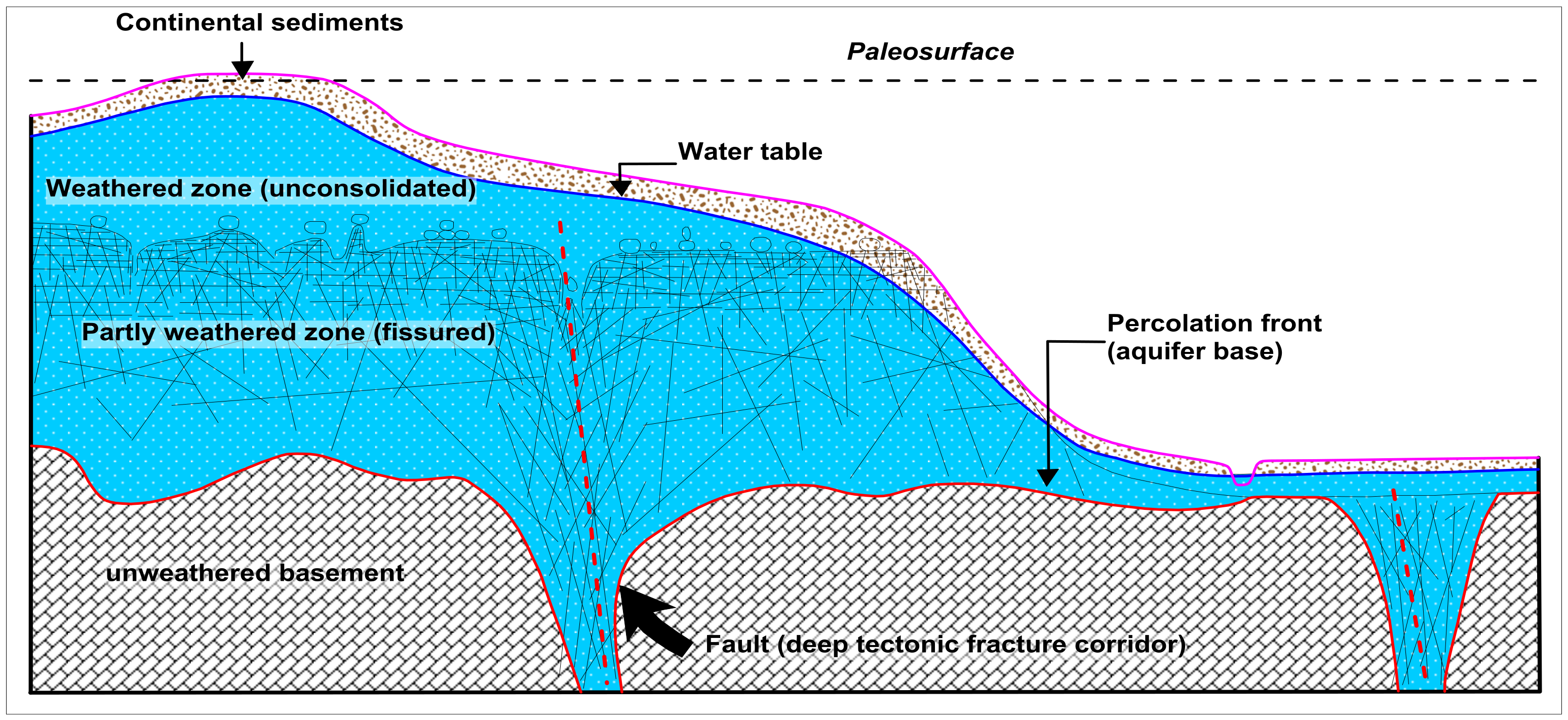
Figure 6.
Conceptual model of hydrogeological properties in weathered basement rock (modified after [54]).
Figure 6.
Conceptual model of hydrogeological properties in weathered basement rock (modified after [54]).

Figure 7.
Water table in the study areawith respect to (a) depth and (b) elevation.
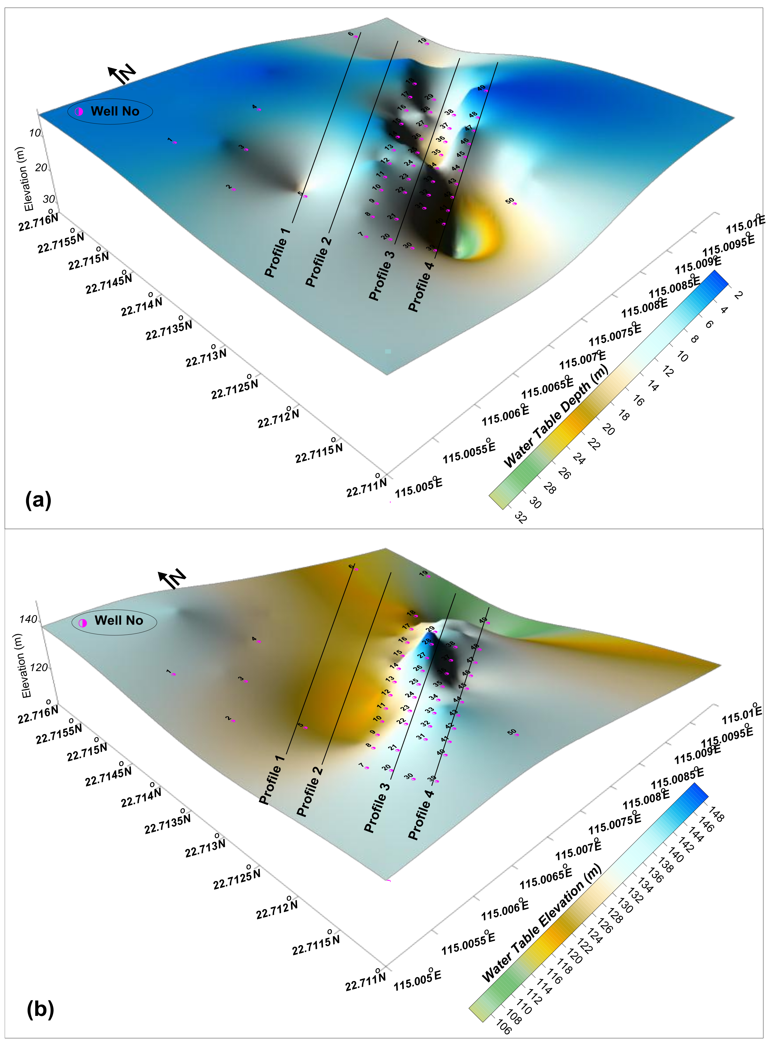
Figure 8.
Electrical image along profile 1 (a) model resistivity with topography (b) interpreted model resistivity with topography.
Figure 8.
Electrical image along profile 1 (a) model resistivity with topography (b) interpreted model resistivity with topography.

Figure 9.
Graphical plots of Joint Profile Method (cross-sectional) along profile 1 for (a, b) resistivity (c, d) self potential and (e, f) induced polarization.
Figure 9.
Graphical plots of Joint Profile Method (cross-sectional) along profile 1 for (a, b) resistivity (c, d) self potential and (e, f) induced polarization.
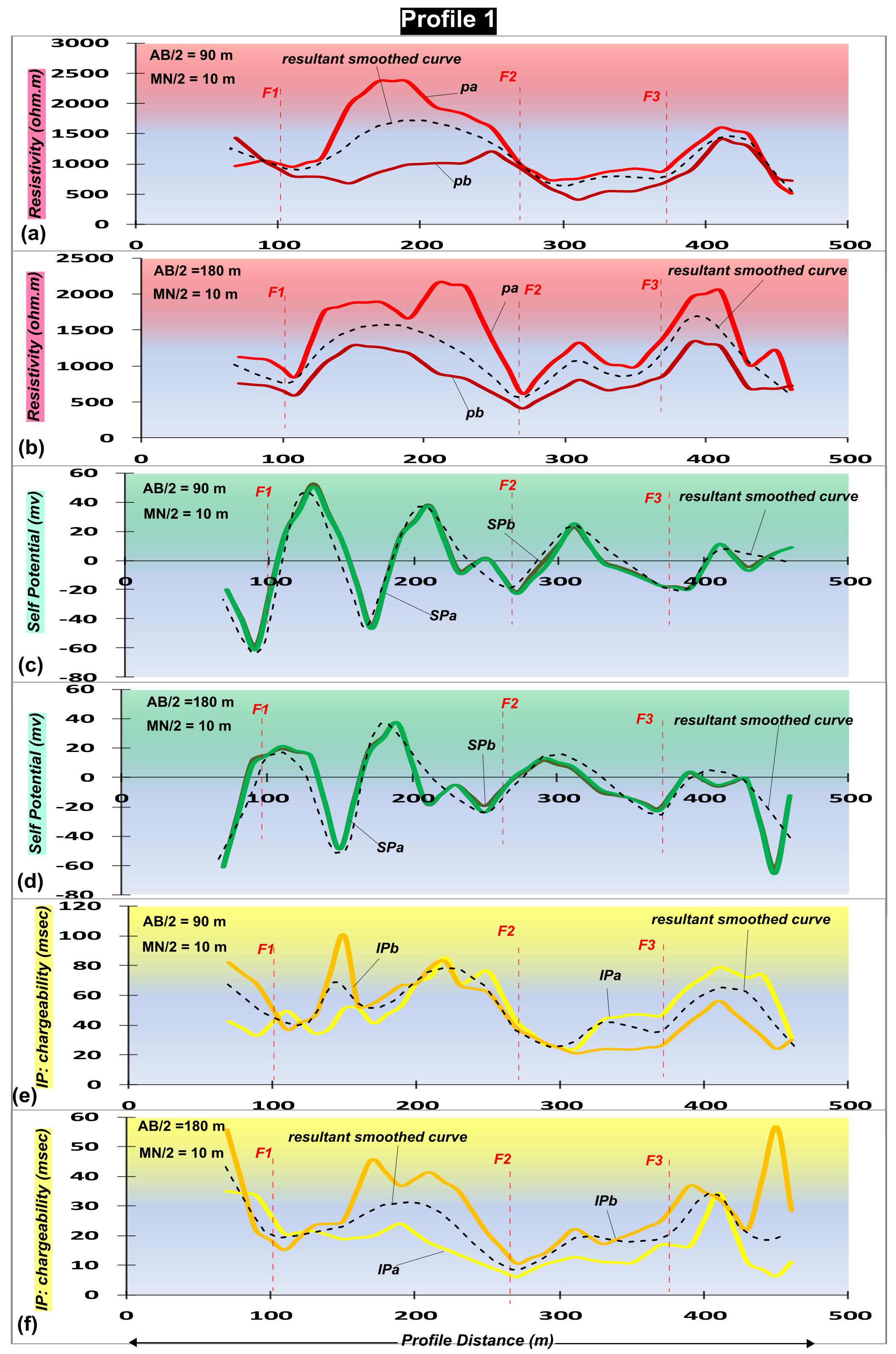
Figure 10.
Electrical image along profile 2 (a) model resistivity with topography (b) interpreted model resistivity with topography.
Figure 10.
Electrical image along profile 2 (a) model resistivity with topography (b) interpreted model resistivity with topography.
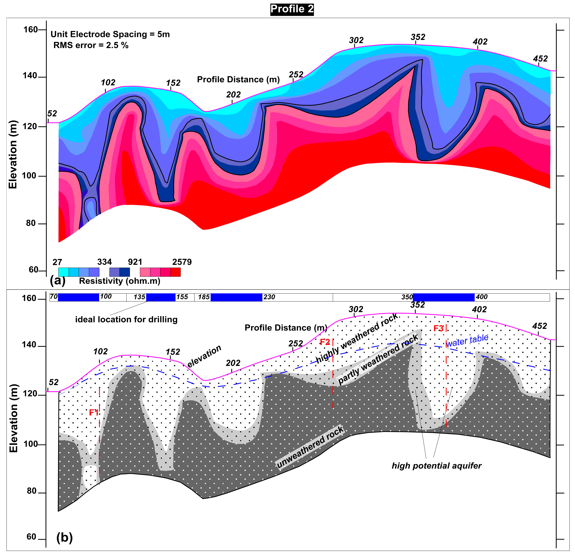
Figure 11.
Electrical image along profile 3 (a) model resistivity with topography (b) interpreted model resistivity with topography.
Figure 11.
Electrical image along profile 3 (a) model resistivity with topography (b) interpreted model resistivity with topography.

Figure 12.
Electrical image along profile 3 (a) model resistivity with topography (b) interpreted model resistivity with topography.
Figure 12.
Electrical image along profile 3 (a) model resistivity with topography (b) interpreted model resistivity with topography.

Figure 13.
Graphical plots of Joint Profile Method (cross-sectional) along profile 4 for (a, b) resistivity (c, d) self potential and (e, f) induced polarization.
Figure 13.
Graphical plots of Joint Profile Method (cross-sectional) along profile 4 for (a, b) resistivity (c, d) self potential and (e, f) induced polarization.

Figure 14.
Graphical plots of magnetic data along (a) profile 1, (b) profile 2, (c) profile 3 and (d) profile 4.
Figure 14.
Graphical plots of magnetic data along (a) profile 1, (b) profile 2, (c) profile 3 and (d) profile 4.

Figure 15.
Map showing the locations of rock and water samples in the investigated area.
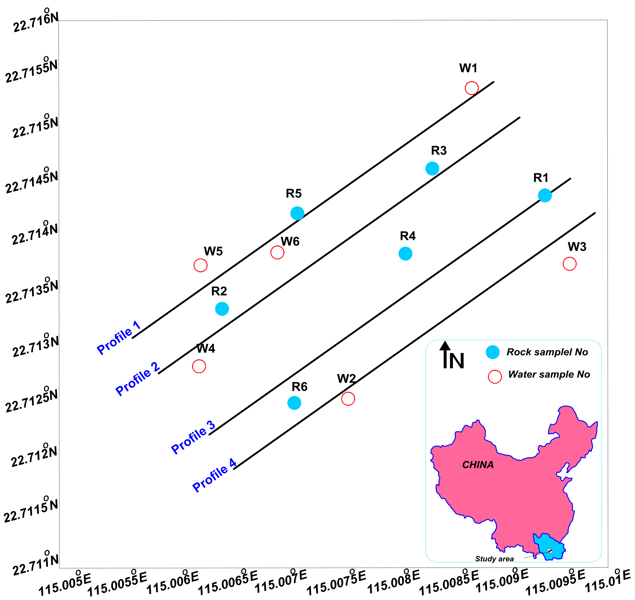
Figure 16.
Graphical representation of weathered-partly weathered, unweathered-partly weathered, water table and topography curves along (a) profile 1, (b) profile 2, (c) profile 3 and (d) profile 4.
Figure 16.
Graphical representation of weathered-partly weathered, unweathered-partly weathered, water table and topography curves along (a) profile 1, (b) profile 2, (c) profile 3 and (d) profile 4.
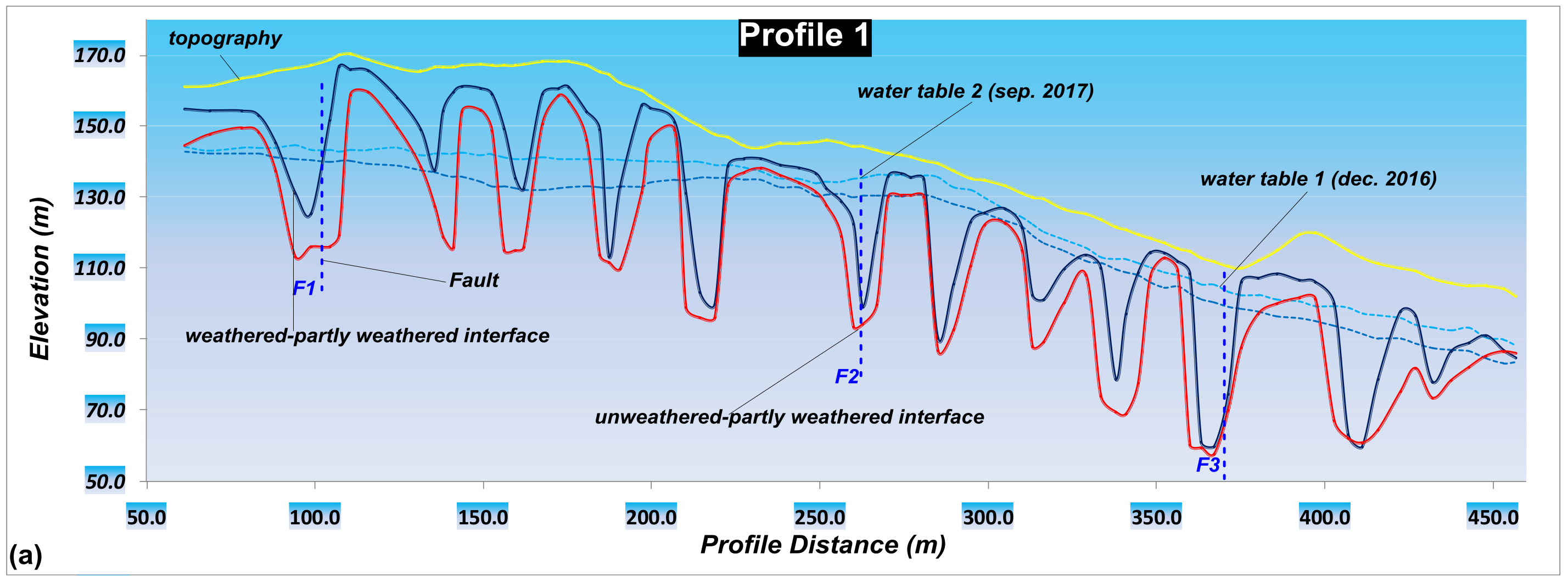
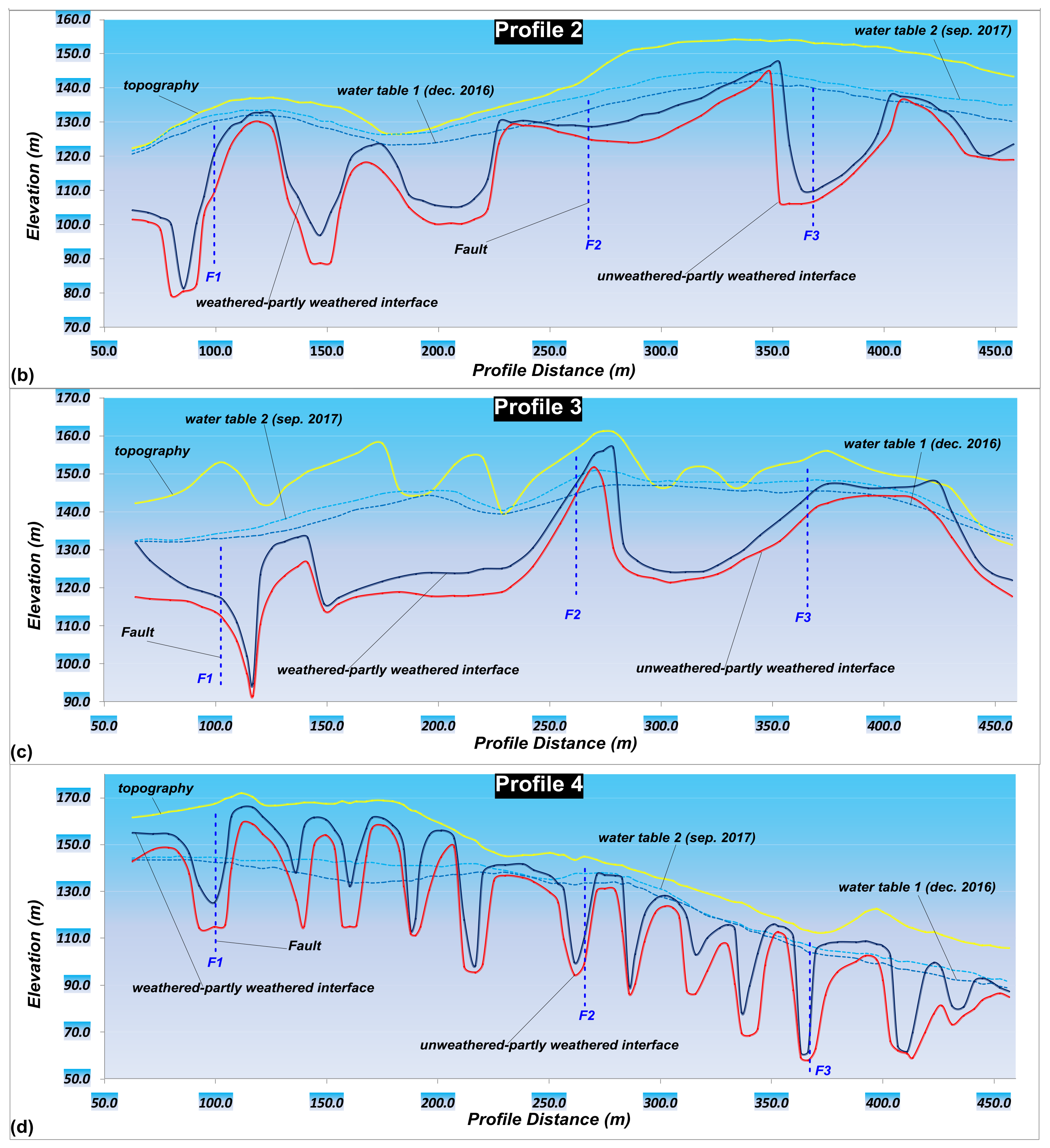
Figure 17.
Interpreted ERT profiles with GW flow direction and faults orientation in the study area.
Figure 17.
Interpreted ERT profiles with GW flow direction and faults orientation in the study area.

Table 1.
Resistivity and lithology calibration in the study area.
| Resistivity of Rock (Ωm) | Type of Rock |
|---|---|
| Below water table and the resistivity between 22 Ωm–345 Ωm | Highly weathered rock |
| Below water table and resistivity between 324 Ωm–926 Ωm | Partly weathered rock |
| Below water table and resistivity greater between 913 Ωm–2579 Ωm | Unweathered rock |
Table 2.
The results of XRD for mineral analysis.
| Rock Sample Number | Description | Major Minerals (>50%) | Secondary Minerals (10–30%) | Minor Minerals (5–10%) |
|---|---|---|---|---|
| 1 (Weathered rock) | Red weathered soil | Quartz | - | Halloysite |
| 2 (Weathered rock) | Yellow weathered soil | Quartz | - | - |
| 3 (Weathered rock) | Earthy fault mud | Quartz | Microcline | Perlite |
| 4 (Weathered rock) | Brown yellow residual soil | Quartz | Kaolinite | - |
| 5 (Bedrock) | Gray black tuff | Quartz | Albite, Zinnwaldite | Sodalite |
| 6 (Bedrock) | Gray black tuff | Quartz | Albite, Zinnwaldite | Ankerite |
Table 3.
The results of physicochemical analysis for groundwater samples.
| Water Sample Number | Parameters | |||||||||||||
| Cations (Measured Concentration in mg/L) | Anions (Measured Concentration in mg/L) | EC (μS/cm) | TDS (mg/L) | pH | Charge Balance Error (%) | |||||||||
| Na+ | K+ | Ca2+ | Mg2+ | NH4+ | Cl− | SO42− | HCO3− | NO3− | ||||||
| 1 | 10.6 | 3.84 | 4.06 | 0.74 | 0.02 | 8.54 | 1.19 | 38.89 | 0.28 | 125 | 68.76 | 7.68 | −4.9 | |
| 2 | 9.8 | 3.07 | 1.62 | 0.49 | 0.02 | 8.54 | 1.81 | 23.93 | 0.16 | 113 | 61.09 | 7.58 | −3.7 | |
| 3 | 13 | 3.11 | 2.84 | 0.49 | 0.02 | 10.68 | 0.94 | 29.91 | 0.10 | 127 | 69.59 | 7.02 | 0.9 | |
| 4 | 11.4 | 3.24 | 2.84 | 1.23 | 0.02 | 9.61 | 1.19 | 35.89 | 0.22 | 140 | 76.30 | 7.28 | −3.7 | |
| 5 | 9.9 | 3.70 | 4.87 | 1.48 | 0.02 | 10.68 | 3.89 | 35.89 | 0.31 | 137 | 74.67 | 7.11 | −4.5 | |
| 6 | 9.5 | 3.68 | 4.74 | 1.45 | 0.02 | 10.88 | 3.23 | 34.23 | 0.32 | 135 | 73.20 | 7.13 | −4.2 | |
| WHO limit for groundwater parameters | ||||||||||||||
| 200 | 55 | 100 | 50 | - | 250 | 200 | 600 | - | 1500 | 1000 | 6.5–8.5 | |||
| Samples exceeding WHO limit [58] | ||||||||||||||
| - | - | - | - | - | - | - | - | - | - | - | - | |||
© 2018 by the authors. Licensee MDPI, Basel, Switzerland. This article is an open access article distributed under the terms and conditions of the Creative Commons Attribution (CC BY) license (http://creativecommons.org/licenses/by/4.0/).
Share and Cite
MDPI and ACS Style
Gao, Q.; Shang, Y.; Hasan, M.; Jin, W.; Yang, P. Evaluation of a Weathered Rock Aquifer Using ERT Method in South Guangdong, China. Water 2018, 10, 293. https://doi.org/10.3390/w10030293
AMA Style
Gao Q, Shang Y, Hasan M, Jin W, Yang P. Evaluation of a Weathered Rock Aquifer Using ERT Method in South Guangdong, China. Water. 2018; 10(3):293. https://doi.org/10.3390/w10030293
Chicago/Turabian StyleGao, Qiang, Yanjun Shang, Muhammad Hasan, Weijun Jin, and Peng Yang. 2018. "Evaluation of a Weathered Rock Aquifer Using ERT Method in South Guangdong, China" Water 10, no. 3: 293. https://doi.org/10.3390/w10030293
Note that from the first issue of 2016, this journal uses article numbers instead of page numbers. See further details here.