Model-Based Evaluation of the Effects of River Discharge Modulations on Physical Fish Habitat Quality

 , , and
Abstract
:1. Introduction
2. Material and Methods
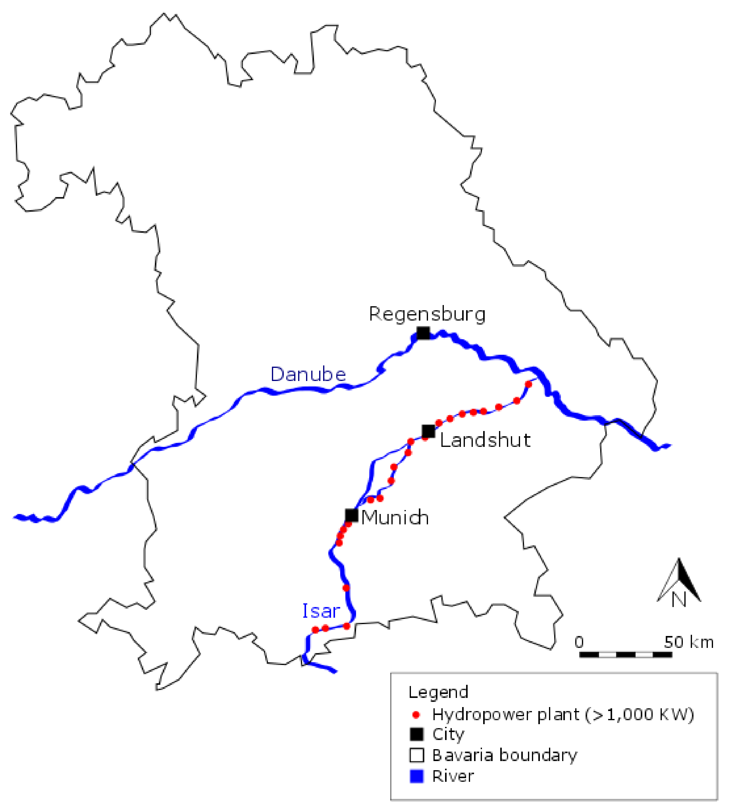
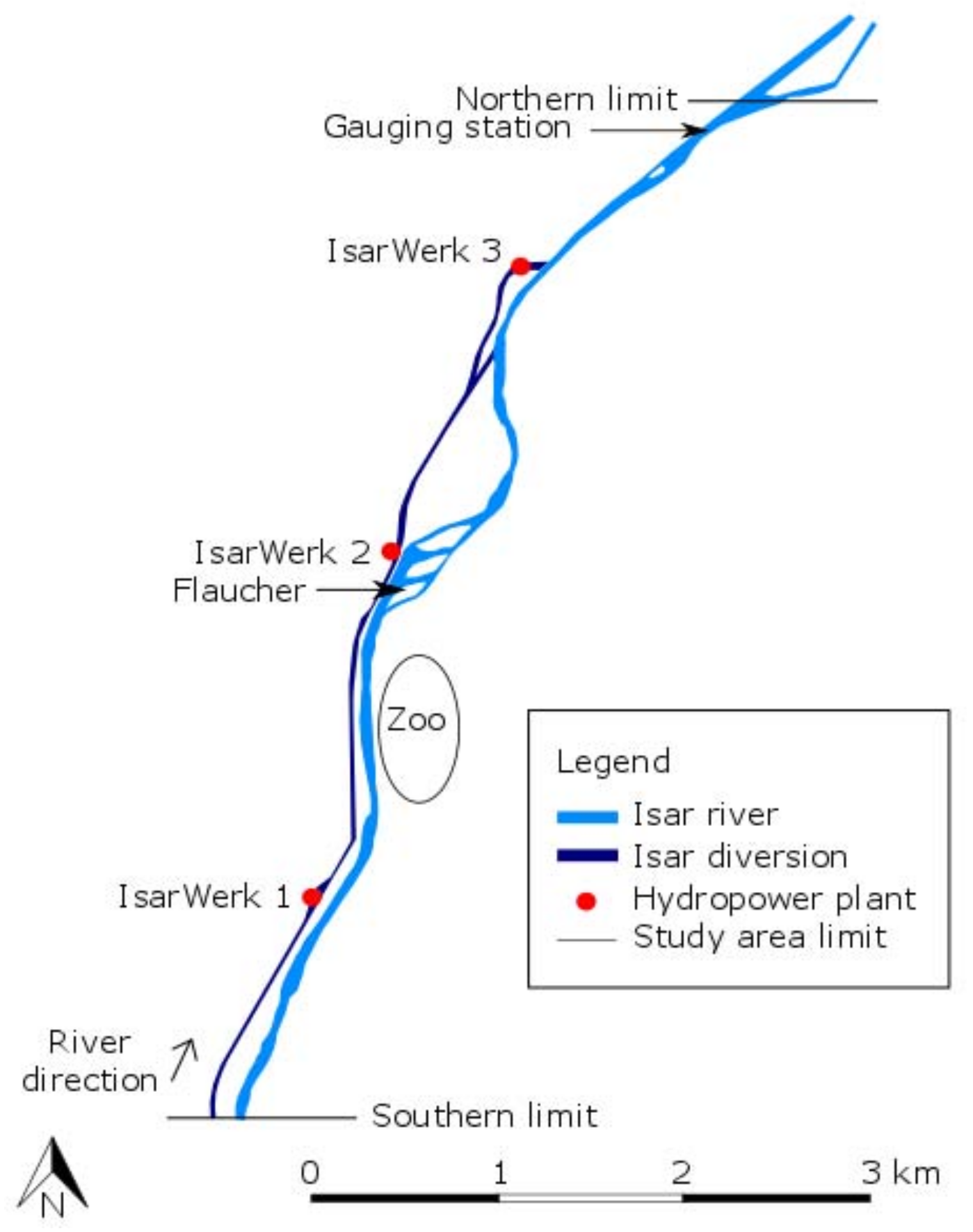
2.1. Study Area
2.2. Physical Characteristics
2.3. Fish Species Studied
2.4. Habitat Model
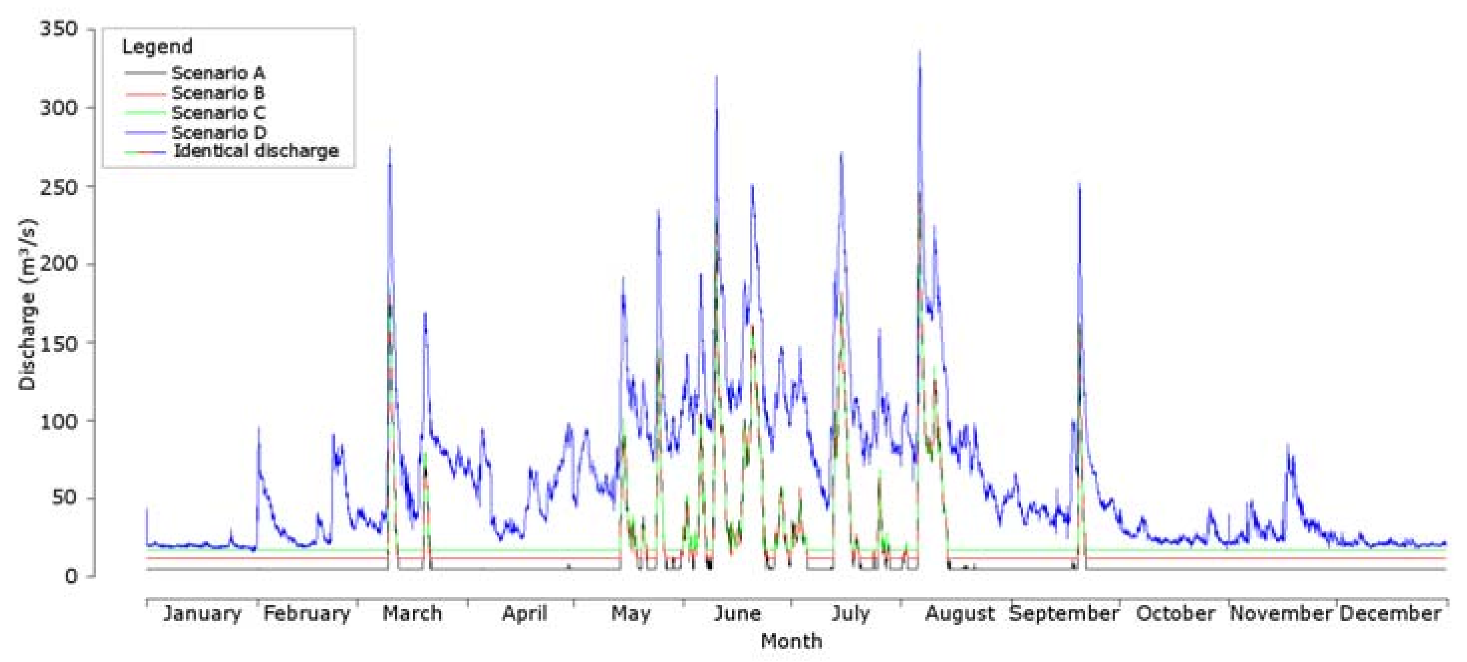
2.5. Data Analysis
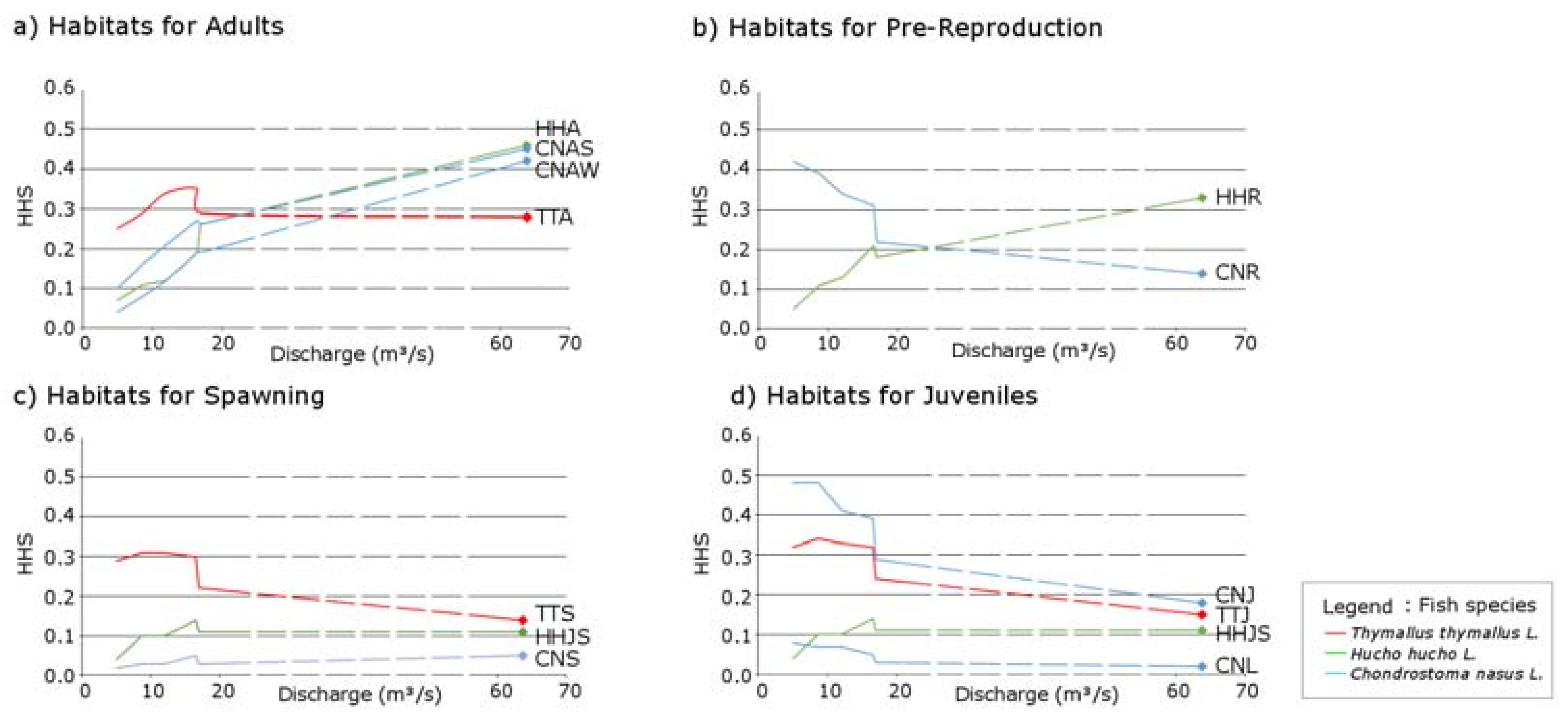
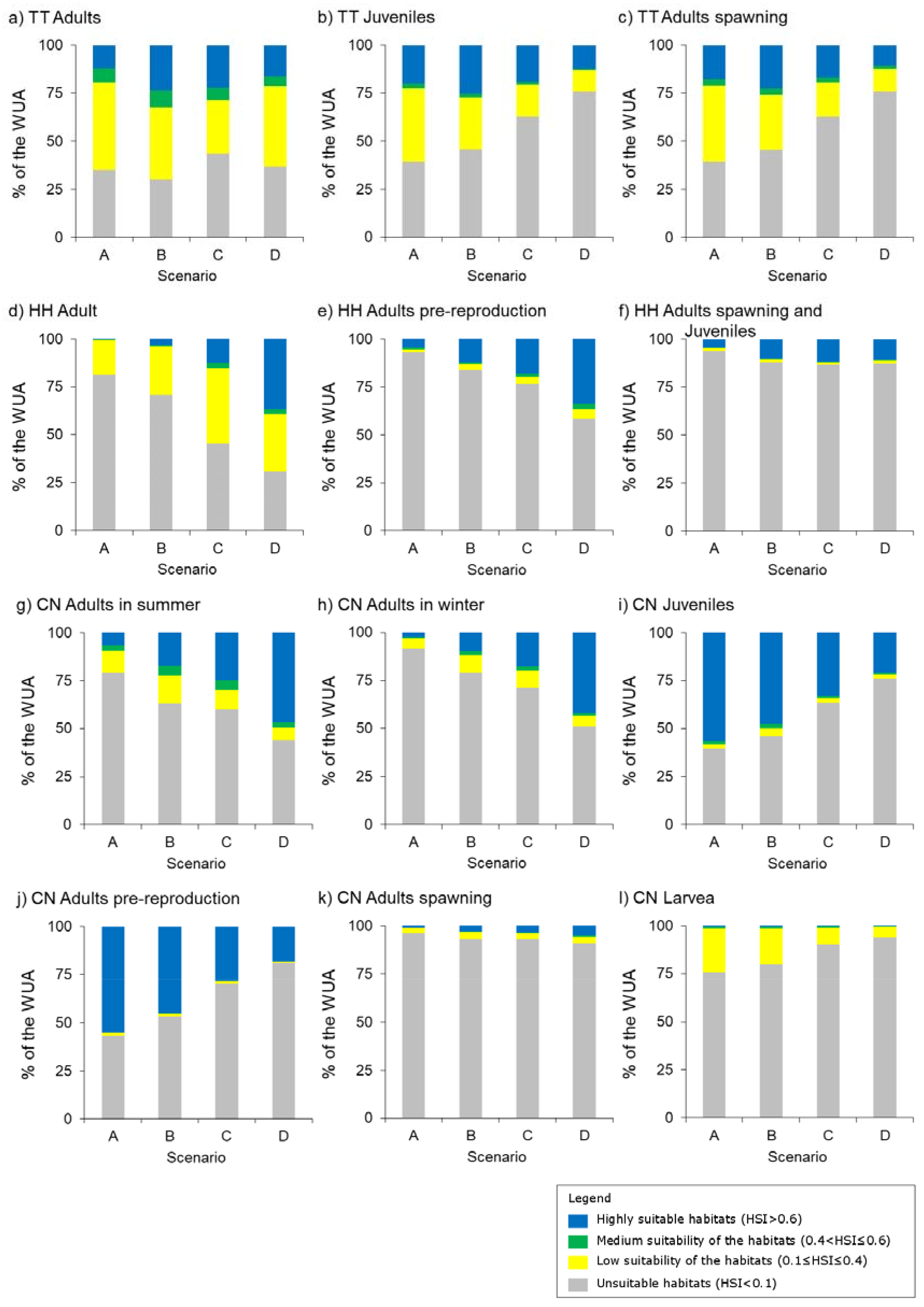
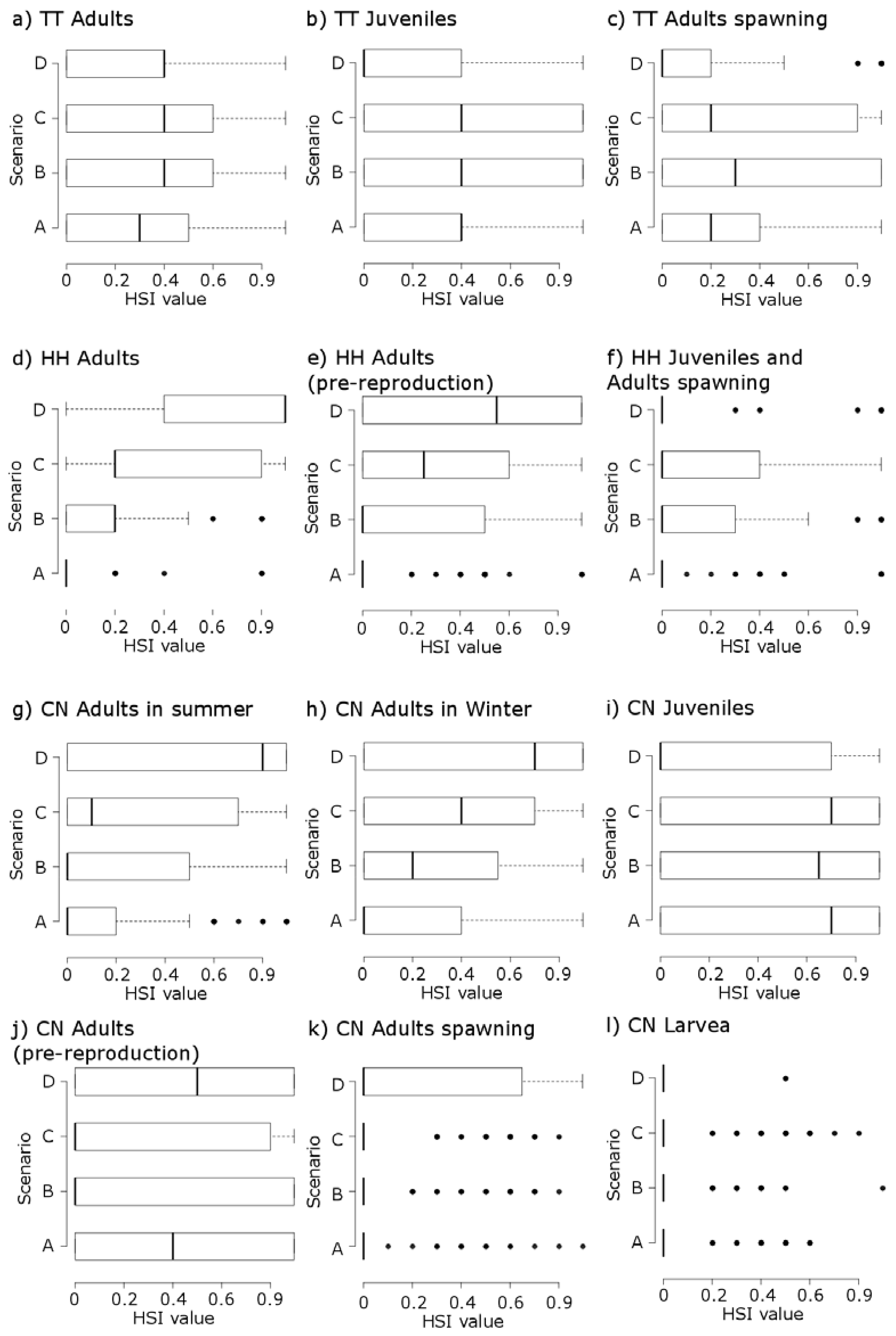
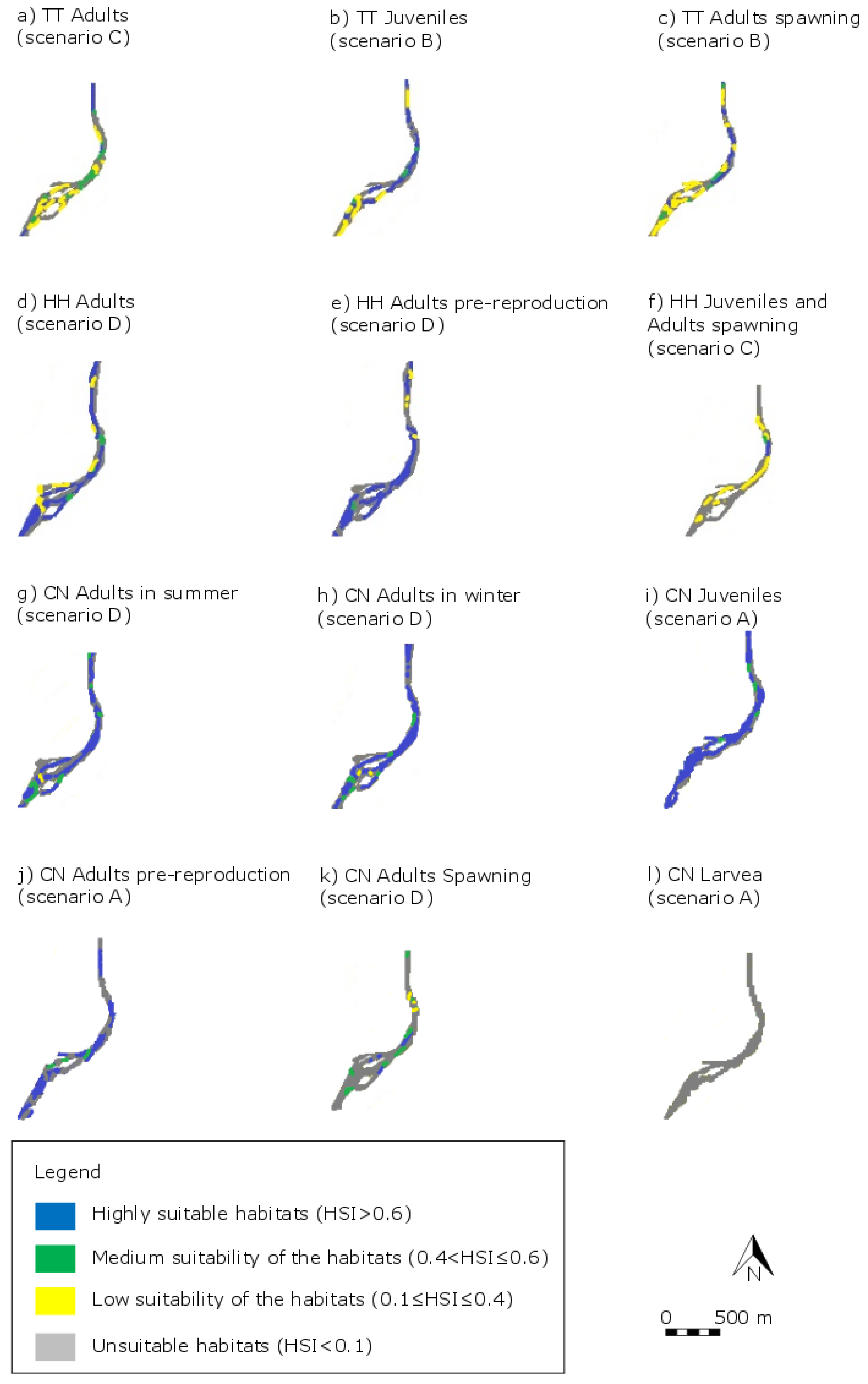
3. Results
3.1. Thymallus thymallus L.
3.2. Hucho hucho L.
3.3. Chondrostoma nasus L.
4. Discussion
4.1. Identification of the Best Scenario
4.2. Habitat Distribution Changes
4.3. Method Discussion
5. Conclusions
Acknowledgments
Author Contributions
Conflicts of Interest
References
- UN. Kyoto Protocol to the United Nations Framework Convention on Climate Change; UN: New York, NY, USA, 1997; Volume 21. [Google Scholar]
- EU. Directive 2009/28/EC of the European Parliament and of the Council of 23 April 2009 on the Promotion of the Use of Energy from Renewable Sources; 2009/28/EC; European Parliament: Brussels, Belgium, 2009; Volume 47. [Google Scholar]
- EIA. International Energy Outlook 2016; EIA: Washington, DC, USA, 2016; Volume 290.
- EURELECTRIC. Hydro in Europe: Powering Renewables; EURELECTRIC: Brussels, Belgium, 2011; Volume 66. [Google Scholar]
- Atilgan, B.; Azapagic, A. Renewable electricity in Turkey: Life cycle environmental impacts. Renew. Energy 2016, 89, 649–657. [Google Scholar] [CrossRef]
- Kollas, I.G.; Mirasgedis, S. Health and Environmental Impacts of Electricity Production from Hydroelectric Power Plants; A a Balkema Publishers: Leiden, The Netherlands, 2000. [Google Scholar]
- Gertsev, V.I.; Gertseva, V.V. A model of sturgeon distribution under a dam of a hydro-electric power plant. Ecol. Model. 1999, 119, 21–28. [Google Scholar] [CrossRef]
- Erskine, W.D.; Terrazzolo, N.; Warner, R.F. River rehabilitation from the hydrogeomorphic impacts of a large hydro-electric power project: Snowy River, Australia. Regul. Rivers Res. Manag. 1999, 15, 3–24. [Google Scholar] [CrossRef]
- Martin, S.M.; Lorenzen, K.; Arthur, R.I.; Kaisone, P.; Souvannalangsy, K. Impacts of fishing by dewatering on fish assemblages of tropical floodplain wetlands: A matter of frequency and context. Biol. Conserv. 2011, 144, 633–640. [Google Scholar] [CrossRef]
- Sauterleute, J.F.; Hedger, R.D.; Hauer, C.; Pulg, U.; Skoglund, H.; Sundt-Hansen, L.E.; Bakken, T.H.; Ugedal, O. Modelling the effects of stranding on the Atlantic salmon population in the Dale River, Norway. Sci. Total Environ. 2016, 573, 574–584. [Google Scholar] [CrossRef] [PubMed]
- Capra, H.; Plichard, L.; Bergé, J.; Pella, H.; Ovidio, M.; McNeil, E.; Lamouroux, N. Fish habitat selection in a large hydropeaking river: Strong individual and temporal variations revealed by telemetry. Sci. Total Environ. 2017, 578, 109–120. [Google Scholar] [CrossRef] [PubMed]
- Hauer, C.; Siviglia, A.; Zolezzi, G. Hydropeaking in regulated rivers—From process understanding to design of mitigation measures. Sci. Total Environ. 2017, 579, 22–26. [Google Scholar] [CrossRef] [PubMed]
- Holzapfel, P.; Leitner, P.; Habersack, H.; Graf, W.; Hauer, C. Evaluation of hydropeaking impacts on the food web in alpine streams based on modelling of fish- and macroinvertebrate habitats. Sci. Total Environ. 2017, 575, 1489–1502. [Google Scholar] [CrossRef] [PubMed]
- Nagrodski, A.; Raby, G.D.; Hasler, C.T.; Taylor, M.K.; Cooke, S.J. Fish stranding in freshwater systems: Sources, consequences, and mitigation. J. Environ. Manag. 2012, 103, 133–141. [Google Scholar] [CrossRef] [PubMed]
- Schülting, L.; Feld, C.K.; Graf, W. Effects of hydro- and thermopeaking on benthic macroinvertebrate drift. Sci. Total Environ. 2016, 573, 1472–1480. [Google Scholar] [CrossRef] [PubMed]
- EU. Directive 2000/60/EC of the European Parliament and of the Council of 23 October 2000 establishing a framework for Community action in the field of water policy. Off. J. (OJ L 327) 2000, 327, 1–73. [Google Scholar]
- Abazaj, J.; Moen, O.; Ruud, A. Striking the Balance between Renewable Energy Generation and Water Status Protection: Hydropower in the context of the European Renewable Energy Directive and Water Framework Directive. Environ. Policy Gov. 2016, 26, 409–421. [Google Scholar] [CrossRef]
- Wagner, B.; Hauer, C.; Schoder, A.; Habersack, H. A review of hydropower in Austria: Past, present and future development. Renew. Sustain. Energy Rev. 2015, 50, 304–314. [Google Scholar] [CrossRef]
- Rutschmann, P.; Sepp, A.; Geiger, F.; Barbier, J. TUM Shaft Hydro Power—Efficient and Ecological. Wasserwirtschaft 2011, 101, 33–36. [Google Scholar] [CrossRef]
- Gebler, R.J.; Lehmann, P. Design of both Near-Natural Running Waters, Bypassing the newly Built Barrage-Plant and the old Hydro Power Plant of RADAG. Wasserwirtschaft 2010, 100, 40–44. [Google Scholar]
- Premstaller, G.; Cavedon, V.; Pisaturo, G.R.; Schweizer, S.; Adami, V.; Righetti, M. Hydropeaking mitigation project on a multi-purpose hydro-scheme on Valsura River in South Tyrol/Italy. Sci. Total Environ. 2017, 574, 642–653. [Google Scholar] [CrossRef] [PubMed]
- Tonolla, D.; Bruder, A.; Schweizer, S. Evaluation of mitigation measures to reduce hydropeaking impacts on river ecosystems—A case study from the Swiss Alps. Sci. Total Environ. 2017, 574, 594–604. [Google Scholar] [CrossRef] [PubMed]
- Arthington, A.H. Environmental Flows—Saving Rivers in the Third Millennium; University of California: Berkeley, CA, USA; Los Angeles, CA, USA, 2012. [Google Scholar]
- Forslund, A.; Renöfält, B.M.; Barchiesi, S.; Cross, K.; Davidson, S.; Farrell, T.; Korsgaard, L.; Krchnak, K.; McClain, M.; Meijer, K.; et al. Securing Water for Ecosystems and Human Well-being: The Importance of Environmental Flows. In World Water Week; Indiana University: Stockholm, Sweden, 2009. [Google Scholar]
- Postel, S.L. Entering an era of water scarcity: The challenges ahead. Ecol. Appl. 2000, 10, 941–948. [Google Scholar] [CrossRef]
- Bakker, K. Water Security: Research Challenges and Opportunities. Science 2012, 337, 914–915. [Google Scholar] [CrossRef] [PubMed]
- Morandi, B. La restauration des cours d’eau en France et à l’étranger: De la définition du concept à l’évaluation de l’action. In Geography; University of Lyon: Lyon, France, 2014; p. 646. [Google Scholar]
- Zingraff-Hamed, A.; Greulich, S.; Pauleit, S.; Wantzen, K.M. Urban and rural river restoration in France: A typology. Restor. Ecol. 2017, 25, 994–1004. [Google Scholar] [CrossRef]
- Mouton, A.; Schneider, M.; Depestele, J.; Goethals, P.; DePauw, N. Fish habitat modelling as a tool for river management. Ecol. Eng. 2007, 29, 305–315. [Google Scholar] [CrossRef]
- Feld, C.K.; da Silva, P.M.; Sousa, J.P.; de Bello, F.; Bugter, R.; Grandin, U.; Hering, D.; Lavorel, S.; Mountford, O.; Pardo, I.; et al. Indicators of biodiversity and ecosystem services: A synthesis across ecosystems and spatial scales. Oikos 2009, 118, 1862–1871. [Google Scholar] [CrossRef]
- Birk, S.; Bonne, W.; Borja, A.; Brucet, S.; Courrat, A.; Poikane, S.; Solimini, A.; van de Bund, W.; Zampoukas, N.; Hering, D. Three hundred ways to assess Europe’s surface waters: An almost complete overview of biological methods to implement the Water Framework Directive. Ecol. Indic. 2012, 18, 31–41. [Google Scholar] [CrossRef]
- Pander, J.; Geist, J. Ecological indicators for stream restoration success. Ecol. Indic. 2013, 30, 106–118. [Google Scholar] [CrossRef]
- Bui, M.D.; Rutschmann, P. Application of a Numerical Model System to Evaluate Sediment Transport and Spawning Habitats for European Graylings in the High Rhine. Wasserwirtschaft 2015, 105, 27–32. [Google Scholar]
- Fletcher, T.D.; Andrieu, H.; Hamel, P. Understanding, management and modeling of urban hydrology and its consequences for receiving waters: A state of the art. Adv. Water Resour. 2013, 51, 261–279. [Google Scholar] [CrossRef]
- Boavida, I.; Santos, J.M.; Ferreira, T.; Pinheiro, A. Barbel habitat alterations due to hydropeaking. J. Hydro-Environ. Res. 2015, 9, 237–247. [Google Scholar] [CrossRef]
- Pisaturo, G.R.; Righetti, M.; Dumbser, M.; Noack, M.; Schneider, M.; Cavedon, V. The role of 3D-hydraulics in habitat modelling of hydropeaking events. Sci. Total Environ. 2017, 575, 219–230. [Google Scholar] [CrossRef] [PubMed]
- Im, D.; Kang, H.; Kim, K.-H.; Choi, S.-U. Changes of river morphology and physical fish habitat following weir removal. Ecol. Eng. 2011, 37, 883–892. [Google Scholar] [CrossRef]
- Shih, S.-S.; Lee, H.-Y.; Chen, C.-C. Model-based evaluations of spur dikes for fish habitat improvement: A case study of endemic species Varicorhinus barbatulus (Cyprinidae) and Hemimyzon formosanum (Homalopteridae) in Lanyang River, Taiwan. Ecol. Eng. 2008, 34, 127–136. [Google Scholar] [CrossRef]
- Yi, Y.; Tang, C.; Yang, Z.; Chen, X. Influence of Manwan Reservoir on fish habitat in the middle reach of the Lancang River. Ecol. Eng. 2014, 69, 106–117. [Google Scholar] [CrossRef]
- Adriaenssens, V.; Baets, B.D.; Goethals, P.L.M.; Pauw, N.D. Fuzzy rule-based models for decision support in ecosystem management. Sci. Total Environ. 2004, 319, 1–12. [Google Scholar] [CrossRef]
- Bovee, K.D. A Guide to Stream Habitat Analysis Using the Instream Flow Invremental Methodology; US Fish and Wildlife Service: Washington, DC, USA, 1982; Volume 273.
- Heggenes, J.; Traaen, T. Downstream migration and critical water velocities in stream channels for fry of four salmonid species. J. Fish Biol. 1988, 32, 717–727. [Google Scholar] [CrossRef]
- Noack, M.; Schneider, M.; Wieprecht, S. The Habitat Modelling System CASiMiR: A Multivariate Fuzzy-Approach and its Applications. In Ecohydraulics: An Integrated Approach; John Wiley & Sons: Hoboken, NJ, USA, 2013; pp. 75–92. [Google Scholar]
- Schneider, M.; Noack, M.; Gebler, T.; Kopecki, I. Handbook for the Habitat Simulation Model CASiMiR; University of Stuttgart: Stuttgart, Germany, 2010. [Google Scholar]
- Schneider, M. Habitat- und Abflussmodellierung für Fließgewässer mit unscharfen Berechnungsansätzen. In Hydraulic Engineering; University of Stuttgart: Stuttgart, Germany, 2001; p. 158. [Google Scholar]
- Jorde, K.; Schneider, M.; Zoellner, F. Analysis of instream habitat quality—Preference functions and fuzzy models. Stoch. Hydraul. 2000, 671–680. [Google Scholar]
- Nujic, M. Hydro_AS-2D—Ein Zweidimensionales Strömungsmodell für die Wasserwirtschaftliche Praxis; Benutzerhandbuch; Ingenieurbüro Reinhard Beck: Rosenheim, Germany, 2009. [Google Scholar]
- Hüber, F. Fische und Fischerei. In Jahrbuch des Vereins zum Schutz der Bergwelt; Dengler & Rauner GmbH: Stuttgart, Germany, 1998; pp. 90–92. [Google Scholar]
- Kottelat, M.; Freyhof, J. Handbook of European Freshwater Fishes; Publications Kottelat, Cornol and Freyhof: Berlin, Germany, 2007. [Google Scholar]
- Freyhof, J. Thymallus thymallus. The IUCN Red List of Threatened Species 2011: e.T21875A9333742. 2011. Available online: http://www.iucnredlist.org/details/21875/0 (accessed on 24 January 2017).
- Nutzel, R.; Krönke, F. Fische in München; Bund Naturschutz in Bayern e.V.: Munich, Germany, 2008. [Google Scholar]
- Schubert, M.; Klein, M.; Leuner, E.; Kraus, G.; Wendt, P.; Born, O.; Hoch, J.; Ring, T.; Silkenat, W.; Speierl, T.; et al. Fischzustandsbericht 2012; LFU: Starnberg, Germany, 2012; Volume 54. [Google Scholar]
- Auer, S.; Zeiringer, B.; Fuhrer, S.; Tonolla, D.; Schmutz, S. Effects of river bank heterogeneity and time of day on drift and stranding of juvenile European grayling (Thymallus thymallus L.) caused by hydropeaking. Sci. Total Environ. 2017, 575, 1515–1521. [Google Scholar] [CrossRef] [PubMed]
- Cattaneo, F.; Grimardias, D.; Carayon, M.; Persat, H.; Bardonnet, A. A multidimensional typology of riverbank habitats explains the distribution of European grayling (Thymallus thymallus L.) fry in a temperate river. Ecol. Freshw. Fish 2014, 23, 527–543. [Google Scholar] [CrossRef]
- Fukuda, S.; De Baets, B.; Waegeman, W.; Verwaeren, J.; Mouton, A.M. Habitat prediction and knowledge extraction for spawning European grayling (Thymallus thymallus L.) using a broad range of species distribution models. Environ. Model. Softw. 2013, 47, 1–6. [Google Scholar] [CrossRef]
- Mallet, J.P.; Lamouroux, N.; Sagnes, P.; Persat, H. Habitat preferences of European grayling in a mediun size stream, the Ain river, France. J. Fish Biol. 2000, 56, 1312–1326. [Google Scholar] [CrossRef]
- Mouton, A.M.; Schneider, M.; Peter, A.; Holzer, G.; Muller, R.; Goethals, P.L.M.; De Pauw, N. Optimisation of a fuzzy physical habitat model for spawning European grayling (Thymallus thymallus L.) in the Aare river (Thun, Switzerland). Ecol. Model. 2008, 215, 122–132. [Google Scholar] [CrossRef]
- Nykanen, M.; Huusko, A. Suitability criteria for spawning habitat of riverine European grayling. J. Fish Biol. 2002, 60, 1351–1354. [Google Scholar] [CrossRef]
- Nykanen, M.; Huusko, A.; Lahti, M. Changes in movement, range and habitat preferences of adult grayling from late summer to early winter. J. Fish Biol. 2004, 64, 1386–1398. [Google Scholar] [CrossRef]
- Riley, W.D.; Pawson, M.G. Habitat use by Thymallus thymallus in a chalk stream and implications for habitat management. Fish. Manag. Ecol. 2010, 17, 544–553. [Google Scholar] [CrossRef]
- Tuhtan, J.A.; Noack, M.; Wieprecht, S. Estimating Stranding Risk due to Hydropeaking for Juvenile European Grayling Considering River Morphology. KSCE J. Civ. Eng. 2012, 16, 197–206. [Google Scholar] [CrossRef]
- Uiblein, F.; Jagsch, A.; Honsig-Erlenburg, W.; Weiss, S. Status, habitat use, and vulnerability of the European grayling in Austrian waters. J. Fish Biol. 2001, 59, 223–247. [Google Scholar] [CrossRef]
- van Leeuwen, C.H.A.; Museth, J.; Sandlund, O.T.; Qvenild, T.; Vollestad, L.A. Mismatch between fishway operation and timing of fish movements: A risk for cascading effects in partial migration systems. Ecol. Evol. 2016, 6, 2414–2425. [Google Scholar] [CrossRef] [PubMed] [Green Version]
- Vehanen, T.; Huusko, A.; Yrjana, T.; Lahti, M.; Maki-Petays, A. Habitat preference by grayling (Thymallus thymallus) in an artificially modified, hydropeaking riverbed: A contribution to understand the effectiveness of habitat enhancement measures. J. Appl. Ichthyol. 2003, 19, 15–20. [Google Scholar] [CrossRef]
- Weiss, S.J.; Kopun, T.; Bajec, S.S. Assessing natural and disturbed population structure in European grayling Thymallus thymallus: Melding phylogeographic, population genetic and jurisdictional perspectives for conservation planning. J. Fish Biol. 2013, 82, 505–521. [Google Scholar] [CrossRef] [PubMed]
- Freyhof, J.; Kottelat, M. Hucho hucho. IUCN Red List of Threatened Species 2008. Available online: http://www.iucnredlist.org/details/10264/0 (accessed on 24 January 2017).
- Holcik, J. Threatened fishes of the world—Hucho hucho (linnaeus, 1758) (Salmonidae). Environ. Biol. Fishes 1995, 43, 105–106. [Google Scholar] [CrossRef]
- EC. Council Directive 92/43/EEC of 21 May 1992 on the Conservation of Natural Habitats and of Wild Fauna and Flora; 92/43/EEC; EC: Brussels, Belgium, 1992; Volume 44. [Google Scholar]
- EC. Convention on the Conservation of European Wildlife and Natural Habitats; EC: Brussels, Belgium, 1979; Volume 12. [Google Scholar]
- Holcik, J. Conservation of the Huchen, Hucho hucho (L.), (Salmonidae) with special reference to slovakian rivers. J. Fish Biol. 1990, 37, 113–121. [Google Scholar] [CrossRef]
- Kottelat, M. European freshwater fishes. Biologia 1997, 52, 1–271. [Google Scholar]
- Jatteau, P. The Huchen (Hucho hucho L.) Review on farming techniques and prospects. Bull. Fr. Peche Piscic. 1991, 322, 97–108. [Google Scholar] [CrossRef]
- Jungwirth, M.; Kossmann, H.; Schmutz, S. Rearing the Danube Salmon (Hucho hucho L.) fry at different temperatures, with particular emphasis on freeze-dried zooplankton as dry feed additive. Aquaculture 1989, 77, 363–371. [Google Scholar] [CrossRef]
- Kucinski, M.; Ocalewicz, K.; Fopp-Bayat, D.; Liszewski, T.; Furgala-Selezniow, G.; Jankun, M. Distribution and Heterogeneity of Heterochromatin in the European Huchen (Hucho hucho Linnaeus, 1758) (Salmonidae). Folia Biol.-Krakow 2014, 62, 81–89. [Google Scholar]
- Nikcevic, M.; Mickovic, B.; Hegedis, A.; Andjus, R.K. Feeding habits of huchen Hucho hucho (Salmonidae) fry in the River Tresnjica, Yugoslavia. Ital. J. Zool. 1998, 65, 231–233. [Google Scholar] [CrossRef]
- Sternecker, K.; Geist, J. The effects of stream substratum composition on the emergence of salmonid fry. Ecol. Freshw. Fish 2010, 19, 537–544. [Google Scholar] [CrossRef]
- Bruslé, J.; Quignard, J.-P. Biologie des Poissons d’eau Douce Européens; Tec&Doc: Lavoisier, Paris, France, 2001. [Google Scholar]
- Freyhof, J. Chondrostoma nasus. 2011. (errata version published in 2016). Available online: http://www.iucnredlist.org/details/4789/0 (accessed on 24 January 2017).
- Reinartz, R. Untersuchungen zur Gefährdungssituation der Fishart Nase (Chondrostoma nasus L.) in bayerischen gewäsern. In Institut für Tierwissenschaften; Technical University of Munich: Munich, Germany, 1997; p. 379. [Google Scholar]
- Hennel, R. Untersuchungen zur Bestandssituation der Fischfauna der Mittleren Isar; TU Munich: Munich, Germany, 1991; p. 222. [Google Scholar]
- Zingraff-Hamed, A.; Noack, M.; Greulich, S.; Schwarzwälder, K.; Wantzen, K.M.; Pauleit, S. Model-based evaluation of conflicts between suitable fish habitats and urban recreational pressure. 2018. under review. [Google Scholar]
- Salski, A. Fuzzy-Sets-Anwendungen in der Umweltforschung. In Fuzzy Logic: Theorie und Praxis, 3. Dortmunder Fuzzy-Tage Dortmund, 7–9 Juni 1993; Reusch, B., Ed.; Springer: Berlin/Heidelberg, Germany, 1993; pp. 13–21. [Google Scholar]
- Jorde, K. Ökologisch Begründete, Dynamische Mindestwasserregelungen bei Ausleitungskraftwerken; University of Stuttgart: Stuttgart, Germany, 1996. [Google Scholar]
- von Riedl, A. Strom-Atlas von Baiern, 1806–1808 (Isar von Tölz bis München); Maximilian Joseph Könige von Baiern München: München, Germany, 1808. [Google Scholar]
- Binder, W. Die Isar (Bayern)—Ein alpiner Wildfluss. In Fließgewässer- und Auenentwicklung: Grundlagen und Erfahrungen; Patt, P.J.H., Ed.; Springer: Berlin/Heidelberg, Germany, 2005; p. 524. [Google Scholar]
- Düchs, J. Wann Wird’s an der Isar Wieder Schön?—Die Renaturierung der Isar in München: Über das Verständnis von Natur in der Großstadt; Herbert Utz Verlag GmbH: Munich, Germany, 2014. [Google Scholar]
- Lepori, F.; Palm, D.; Brännäs, E.; Malmqvist, B. Does restoration of structural heterogeneity in streams enhance fish and macroinvertebrate diversity? Ecol. Appl. 2005, 15, 2060–2071. [Google Scholar] [CrossRef]
- Pander, J.; Geist, J. Seasonal and spatial bank habitat use by fish in highly altered rivers—A comparison of four different restoration measures. Ecol. Freshw. Fish 2010, 19, 127–138. [Google Scholar] [CrossRef]
- Bernhardt, E.S.; Palmer, M.A. Restoring streams in an urbanizing world. Freshw. Biol. 2007, 52, 738–751. [Google Scholar] [CrossRef]
- Lobbrecht, A.H. Dynamic Water-System Control—Design and Operation of Regional Water-Ressources Systems; A.A.Balkema: Rotterdam, The Netherland, 1997. [Google Scholar]
- Wantzen, K.M.; Junk, W.J.; Rothhaupt, K.O. An extension of the floodpulse concept (FPC) for lakes. Hydrobiologia 2008, 613, 151–170. [Google Scholar] [CrossRef]
- Junk, W.J.; Wantzen, K.M. The Flood Pulse Concept: New Aspects Approaches and Applications—An Update. In Proceedings of the Second International Symposium on the Management of Large Rivers for Fisheries, Phnom Penh, Kingdom of Cambodia, 11–14 February 2003; Petr, R.L.W.T., Ed.; RAP Publication: Bangkok, Tailand, 2004; pp. 117–140. [Google Scholar]
- Junk, W.J.; Wantzen, K.M. Flood pulsing and the development and maintenance of biodiversity in floodplains. In Ecology of Freshwater and Estuarine Wetlands; Batzer, D.P., Sharitz, R.R., Eds.; University of California Press: Berkeley, CA, USA, 2006; pp. 407–435. [Google Scholar]
- EC. CIS Guidance Document No. 31—Ecological Flows in the Implementation of the Water Framework Directive; European Union: Brussels, Belgium, 2015. [Google Scholar]
- Poff, N.L.; Allan, J.D.; Bain, M.B.; Karr, J.R.; Richter, B.; Sparks, R.; Stromberg, J. The natural flow regime: A new paradigm for riverine conservation and restoration. Bioscience 1997, 47, 769–784. [Google Scholar] [CrossRef]
- Bunn, S.E.; Arthington, A.H. Basic principles and ecological consequences of altered flow regimes for aquatic biodiversity. Environ. Manag. 2002, 30, 492–507. [Google Scholar] [CrossRef]
- Kappus, B.M.; Jansen, W.; Bohmer, J.; Rahmann, H. Historical and present distribution and recent habitat use of nase, Chondrostoma nasus, in the lower Jagst River (Baden-Wurttemberg, Germany). Folia Zool. 1997, 46, 51–60. [Google Scholar]
- Keith, P.; Persat, H.; Feunteun, E.; Allardi, J. Les Poissons D’eau Douce en France; Publication Scientifique du Musée: Paris, France, 2011. [Google Scholar]
- Żarski, D.; Targońska, K.; Ratajski, S.; Kaczkowski, Z.; Kucharczy, D. Reproduction of Nase, Chondrostoma Nasus (L.), Under Controlled Conditions. Arch. Pol. Fish. 2008, 16, 355–362. [Google Scholar]
- Maier, K.J. On the nase, Chondrostoma nasus spawning area situation in Switzerland. Folia Zool. 1997, 46, 79–88. [Google Scholar]
- Noack, M.; Schneider, M. Impacts of Hydropeaking on juvenile fish habitats: A qualitative and quantitative evaluation using the habitat model CASiMiR. In Proceedings of the 7th International Symposium on Ecohydraulics, Concepcion, Chile, 12–16 January 2009. [Google Scholar]
- Perry, A.L.; Low, P.J.; Ellis, J.R.; Reynolds, J.D. Climate Change and Distribution Shifts in Marine Fishes. Science 2005, 308, 1912–1915. [Google Scholar] [CrossRef] [PubMed]
- Wagner, T.; Themessl, M.; Schuppel, A.; Gobiet, A.; Stigler, H.; Birk, S. Impacts of climate change on stream flow and hydro power generation in the Alpine region. Environ. Earth Sci. 2017, 76, 22. [Google Scholar] [CrossRef]
- Lise, W.; van der Laan, J. Investment needs for climate change adaptation measures of electricity power plants in the EU. Energy Sustain. Dev. 2015, 28, 10–20. [Google Scholar] [CrossRef]
- DKRZ. Rechnungen im Rahmen des Internationalen Klimamodell-Vergleichsprojektes CMIP5 und für den Fünften Klimasachstandsbericht der Vereinten Nationen (IPCC AR5). 2017. Available online: https://www.dkrz.de/Klimaforschung/konsortial/ipcc-ar5/ergebnisse/niederschlag (accessed on 5 November 2017).
- Glogger, B. Heisszeit: Klimaänderungen und Naturkatastrophen in der Schweiz; Hochschulverlag AG: Zürich, Switzerland, 1998. [Google Scholar]
- Van Vuuren, D.P.; Edmonds, J.; Kainuma, M.; Riahi, K.; Thomson, A.; Hibbard, K.; Hurtt, G.C.; Kram, T.; Krey, V.; Lamarque, J.-F.; et al. The representative concentration pathways: An overview. Clim. Chang. 2011, 109, 5–31. [Google Scholar] [CrossRef]
- Beckers, F.; Noack, M.; Wieprecht, S. Reliability analysis of a 2D sediment transport model: An example of the lower river Salzach. J. Soils Sediments 2017, 1–12. [Google Scholar] [CrossRef]
- Noack, M.; Ortlepp, J.; Wieprecht, S. An approach to simulate interstitial habitat conditions during the incubation phase of gravel-spawning fish. River Res. Appl. 2016, 33, 192–201. [Google Scholar] [CrossRef]
- Noack, M. Modelling approach for interstitial sediment dynamics and reproduction of gravel-spawning fish—Simulation der interstitialen Sedimentdynamik und der Reproduktion kieslaichender Fischarten. In Institut für Wasser- und Umweltsystemmodellierung; Universität Stuttgart: Stuttgart, Germany, 2012. [Google Scholar]
- Dufour, S.; Piégay, H. From the Myth of a Lost Paradise to Targeted River Restoration: Forget Natural References and Focus on Human Benefits. River Res. Appl. 2009, 24, 1–14. [Google Scholar] [CrossRef]
- Choi, Y.D. Theories for ecological restoration in changing environment: Toward ‘futuristic’ restoration. Ecol. Res. 2004, 19, 75–81. [Google Scholar] [CrossRef]
- Wantzen, K.M.; Ballouche, A.; Longuet, I.; Bao, I.; Bocoum, H.; Cissé, L.; Chauhan, M.; Girard, P.; Gopal, B.; Kane, A.; et al. River Culture: An eco-social approach to mitigate the biological and cultural diversity crisis in riverscapes. Ecohydrol. Hydrobiol. 2016, 16, 7–18. [Google Scholar] [CrossRef]


| Fish Species | Habitat Type | Life Cycle Stage | Season | Water Velocity | Water Depth | Substratum |
|---|---|---|---|---|---|---|
| Thymallus thymallus | TTA | Adults | All | Moderate to high (0.7–1.1 m/s) | High (100–140 cm) | Medium to fine-grained substratum |
| TTS | Adults spawning | Spring (January–April) | Very low (0.2–0.4 m/s) | Low to very high (10 cm–230 cm) | Fine-grained substratum | |
| TTJ | Juveniles | All | Moderate to high (0.7–1.1 m/s) | Moderate (50–80 cm) | Fine-grained to medium substratum | |
| Hucho hucho | HHA | Adults | All | Moderate to very high (>0.7 m/s) | High (>100 cm) | Fine-grained to medium substratum |
| HHR | Adults (pre-reproduction) | Spring (February–April) | High to very high (>1.0 m/s) | Moderate to high (30–150 cm) | Medium gravel to large stones | |
| HHSJ | Adults spawning | Spring (February–May) | High to very high (>1.0 m/s) | Moderate (20–60 cm) | Medium gravel | |
| and Juveniles | All | |||||
| Chondrostoma nasus | CNS | Spawning | Spring (March–May) | High (1.0–1.5 m/s) | Moderate (20–40 cm) | Medium to fine-grained substratum |
| CNL | Larvae | Spring | Low (0.5–0.7 m/s) | Low (5–10 cm) | Fine-grained substratum | |
| CNJ | Juveniles | All | Low (under 0.6 m/s) | Low (5–20 cm) | Coarse substratum | |
| CNAW | Adults | Winter | High (1.0–1.5 m/s) | High (1–2 m) | Variable substratum | |
| CNR | Adults (pre-reproduction) | Spring (February–May) | Low to very low (less than 0.7 m/s) | Moderate (20–40 cm) | Medium gravel to large stones | |
| CNAS | Adults | Summer | Moderate to high (0.7 to 1.5 m/s) | Moderate (20–50 cm) | Rock to gravel |
| Linguistic Modalities | Velocity | Water Depth | Substratum |
|---|---|---|---|
| Very low | 0–0.4 m/s (±0.1 m/s) | 0–0.1 m (±5 cm) | Organic matter |
| Low | 0.5–0.7 m/s (±0.1 m/s) | 0.1–0.2 m (±5 cm) | Sand < 6 mm |
| Medium | 0.75–0.9 m/s (±0.1 m/s) | 0.2 (±5 cm) to 0.5 (±10 cm) | Gravel from 6 to 120 mm |
| High | 1 m/s (±0.15 m/s) to 1.5 m/s (±0.25 m/s) | 0.5 (±10 cm) to 1.15 m (±25 cm) | Large stones 12–20 cm |
| Very high | Start at 1.75 m/s (±0.25 m/s) | Start at 1.25 (±25 cm) | Boulders > 20 cm, Rock |
| Velocity | Depth | Substrate | HSI | Example |
|---|---|---|---|---|
| M | H | VH | VL | Rule 1: IF velocity ‘Medium’ AND depth ‘High’ AND substratum ‘Very high’ THEN HSI ‘Very low’ |
| M | H | H | H | Rule 2: IF velocity ‘Medium’ AND depth ‘High’ AND substratum ‘High’ THEN HSI ‘High’ |
| M | H | M | VH | Rule 3: IF velocity ‘Medium’ AND depth ‘High’ AND substratum ‘Medium’ THEN HSI ‘Very high’ |
| M | M | H | M | Rule 4: IF velocity ‘Medium’ AND depth ‘Medium’ AND substratum ‘High’ THEN HSI ‘Medium’ |
| M | M | M | H | Rule 5: IF velocity ‘Medium’ AND depth ‘Medium’ AND substratum ‘Medium’ THEN HSI ‘High’ |
| Fish species | Life cycle stage (Habitat types) | Indicators | Scenario | |||
|---|---|---|---|---|---|---|
| A | B | C | D | |||
| Thymallus thymallus | Adults (TTA) | WUA (1,000 m²) | 183 | 274 | 276 | 233 |
| HHS | 0.25 | 0.34 | 0.29 | 0.28 | ||
| Mean HSI | Low | Low | Medium | Low | ||
| Spawning (TTS) | WUA (1,000 m²) | 212 | 255 | 210 | 121 | |
| HHS | 0.29 | 0.31 | 0.22 | 0.14 | ||
| Mean HSI | Low | Low | Medium | Very low | ||
| Juveniles (TTJ) | WUA (1,000 m²) | 229 | 270 | 222 | 128 | |
| HHS | 0.32 | 0.33 | 0.24 | 0.15 | ||
| Mean HSI | Low | Low | Low | Very low | ||
| Hucho hucho | Adults (HHA) | WUA (1,000 m²) | 48 | 94 | 243 | 384 |
| HHS | 0.07 | 0.12 | 0.26 | 0.46 | ||
| Mean HSI | Very low | Low | Low | High | ||
| Adults pre-reproduction (HHR) | WUA (1,000 m²) | 35 | 102 | 171 | 277 | |
| HHS | 0.05 | 0.13 | 0.18 | 0.33 | ||
| Mean HSI | Very low | Very low | Very low | Medium | ||
| Spawning and Juveniles (HHJS) | WUA (1,000 m²) | 31 | 79 | 104 | 88 | |
| HHS | 0.04 | 0.10 | 0.11 | 0.11 | ||
| Mean HSI | Very low | Very low | Low | Very low | ||
| Chondrostoma nasus | Adults during the summer (CNAS) | WUA (1,000 m²) | 72 | 167 | 241 | 377 |
| HHS | 0.10 | 0.21 | 0.26 | 0.45 | ||
| Mean HSI | Low | Low | Low | Medium | ||
| Adults during the winter (CNAW) | WUA (1,000 m²) | 30 | 100 | 182 | 355 | |
| HHS | 0.04 | 0.12 | 0.19 | 0.42 | ||
| Mean HSI | Low | Low | Medium | Medium | ||
| Adults pre-reproduction (CNR) | WUA (1,000 m²) | 300 | 277 | 207 | 118 | |
| HHS | 0.42 | 0.34 | 0.22 | 0.14 | ||
| Mean HSI | Medium | Low | Low | Medium | ||
| Juvenils (CNJ) | WUA (1,000 m²) | 341 | 330 | 268 | 153 | |
| HHS | 0.48 | 0.41 | 0.29 | 0.18 | ||
| Mean HSI | Medium | Medium | Medium | Low | ||
| Spawning (CNS) | WUA (1,000 m²) | 11 | 27 | 32 | 39 | |
| HHS | 0.02 | 0.03 | 0.03 | 0.05 | ||
| Mean HSI | Very low | Very low | Very low | Low | ||
| Larvae (CNL) | WUA (1,000 m²) | 60 | 57 | 31 | 18 | |
| HHS | 0.08 | 0.07 | 0.03 | 0.02 | ||
| Mean HSI | Very low | Very low | Very low | Very low | ||
© 2018 by the authors. Licensee MDPI, Basel, Switzerland. This article is an open access article distributed under the terms and conditions of the Creative Commons Attribution (CC BY) license (http://creativecommons.org/licenses/by/4.0/).
Share and Cite
Zingraff-Hamed, A.; Noack, M.; Greulich, S.; Schwarzwälder, K.; Pauleit, S.; Wantzen, K.M. Model-Based Evaluation of the Effects of River Discharge Modulations on Physical Fish Habitat Quality. Water 2018, 10, 374. https://doi.org/10.3390/w10040374
Zingraff-Hamed A, Noack M, Greulich S, Schwarzwälder K, Pauleit S, Wantzen KM. Model-Based Evaluation of the Effects of River Discharge Modulations on Physical Fish Habitat Quality. Water. 2018; 10(4):374. https://doi.org/10.3390/w10040374
Chicago/Turabian StyleZingraff-Hamed, Aude, Markus Noack, Sabine Greulich, Kordula Schwarzwälder, Stephan Pauleit, and Karl M. Wantzen. 2018. "Model-Based Evaluation of the Effects of River Discharge Modulations on Physical Fish Habitat Quality" Water 10, no. 4: 374. https://doi.org/10.3390/w10040374