Experimental and Numerical Investigation of Pre-Breaking and Breaking Vorticity within a Plunging Breaker

Abstract

The characteristics of vorticity induced just prior and at the splash-down of a plunging breaker on a 1:10 planar slope have been studied using wave flume experiments and numerical simulations. Laboratory experiments involved detailed measurements in the outer surf zone of both fluid velocities below trough level, achieved by a fibre-optic laser-Doppler anemometer, and water surface elevations, obtained by an ultrasound probe. A Weakly-Compressible Smoothed Particle (WCSPH) model, coupled with a two-equation model for turbulent stresses, has been employed for the numerical simulations. A thorough calibration of the SPH’s numerical parameters has been first performed, through comparison between numerical and experimental wave elevation and velocity data. Then, considering that time-averaged laboratory data shows a significant vorticity beneath the free surface in the wave pre-breaking region, the vorticity generation mechanism has been thoroughly analyzed by means of the numerical model. In the attempt of explaining the generation of vorticity as induced by flow separation, we also inspected the role of the streamwise flow deceleration and surface-parallel vorticity flux. In analogy with the case of spilling breakers a cause-effect relation has been observed between streamwise flow deceleration and vorticity generation. Numerical findings are positively confirmed by the experimental results.

1. Introduction

Turbulence and undertow currents play an important role in surf-zone mixing and transport processes; therefore, their study is fundamental for the understanding of nearshore dynamics and the related planning and management of coastal engineering activities.

Pioneering studies were carried out by [1,2,3], who qualitatively described the features of plunging breakers in the outer region of the surf zone. More detailed information on the velocity field under plunging breakers can be found in the experimental works by, among others, refs. [4,5,6,7] and more recently by [8,9,10]. In these works, single-point measurement techniques, such as hot-wire anemometry and Laser Doppler Anemometry, were used to provide maps of the flow field in a time-averaged or ensemble-averaged sense.

The advent of non-intrusive measuring techniques, such as Particle Image Velocimetry (PIV) provided accurate and detailed instantaneous spatial maps of the flow field. Moreover, by correlating spatial gradients of the measured velocity components, the instantaneous vorticity maps could be deduced.

Measurements of vorticity using planar PIV were obtained, among others, by [11], who carried out experiments on waves breaking on a submerged breakwater on a 1:100 sloped beach, and by [12], who gained information on the overall characteristics of the 2D flow field of breaking waves in shallow water and proved the existence of oblique descending vortices, previously observed by [13]. An extensive investigation on the surf-zone of breaking waves over a sloping beach, also performed with a PIV, was carried out by [14], who estimated the longshore vorticity. A volumetric particle-tracking system was used by [15] to study the vorticity dynamics during wave breaking on a fixed bar on a rigid plane slope.

Many attempts have been made to identify and examine the source of vorticity in breaking waves [16,17], especially for the case of the spilling waves [18], which most commonly occur, but this topic is still debated and deserves further study. In the breaking wave, the main region of vorticity generation is at the free surface, while seabed vorticity is much smaller. Longuet-Higgins [19] explained this vorticity generation in terms of the combined effect of surface curvature and zero-shear stress boundary conditions at the interface, with a Stokes layer initially confining the generated vorticity, which in a subsequent stage escapes and fills the domain. Also, Lin and Rockwell [20] attributed the vorticity generation to the sharp curvature of the interface, where a flow separation occurs. Complementary to these findings, Dabiri and Gharib [21] experimentally deduced that the major source of vorticity in spilling breakers was attributable to the free surface fluid deceleration before breaking, together with an increase of fluid pressure on the back of the wave, pushing the crest.

What is clear is the fundamental link between near-surface vorticity generation and the subsequent degeneration into the near-surface turbulence of a breaking wave. The mechanism governing this connection still needs a thorough analysis, especially for the lesser investigated plunging breakers. In particular, the vorticity field by a plunging breaker has received less attention than that due to a spiller because spilling waves are representative of storm waves and of bore jumps, thus they frequently occur. However, the same spilling breaker may be regarded as a locally (at wave crest) weak plunging breaker, with the rotational flow generated by the plunger spreading down along the front of the wave and forming a roller [16]. The added value of our study with respect to previous investigations is our focusing on the plunging breaking wave, where the high curvature due to the steepening of the wave and the related flow shearing naturally induce a strong vorticity and related turbulence.

In the perspective to investigate these aspects, numerical models represent a useful tool: the dynamics of breaking-induced mean vorticity was numerically analysed by numerous authors, including [22,23]. If grid-based numerical methods can suffer from certain limitations when used to study such violent free surface flows, particle meshless methods have instead the potential to provide a comprehensive description of the full processes associated with wave breaking, whilst they can accurately capture the water surface profile during such processes.

Among the meshless methods, Smoothed Particle Hydrodynamics (SPH) is at present effective in solving several fluid-dynamic problems with highly nonlinear deformation, such as wave breaking and impact [24,25]; hydraulic jumps [26,27,28,29]; long waves, e.g., floods, tsunamis and landslide submersions [30]; oscillating jets inducing breaking waves [31].

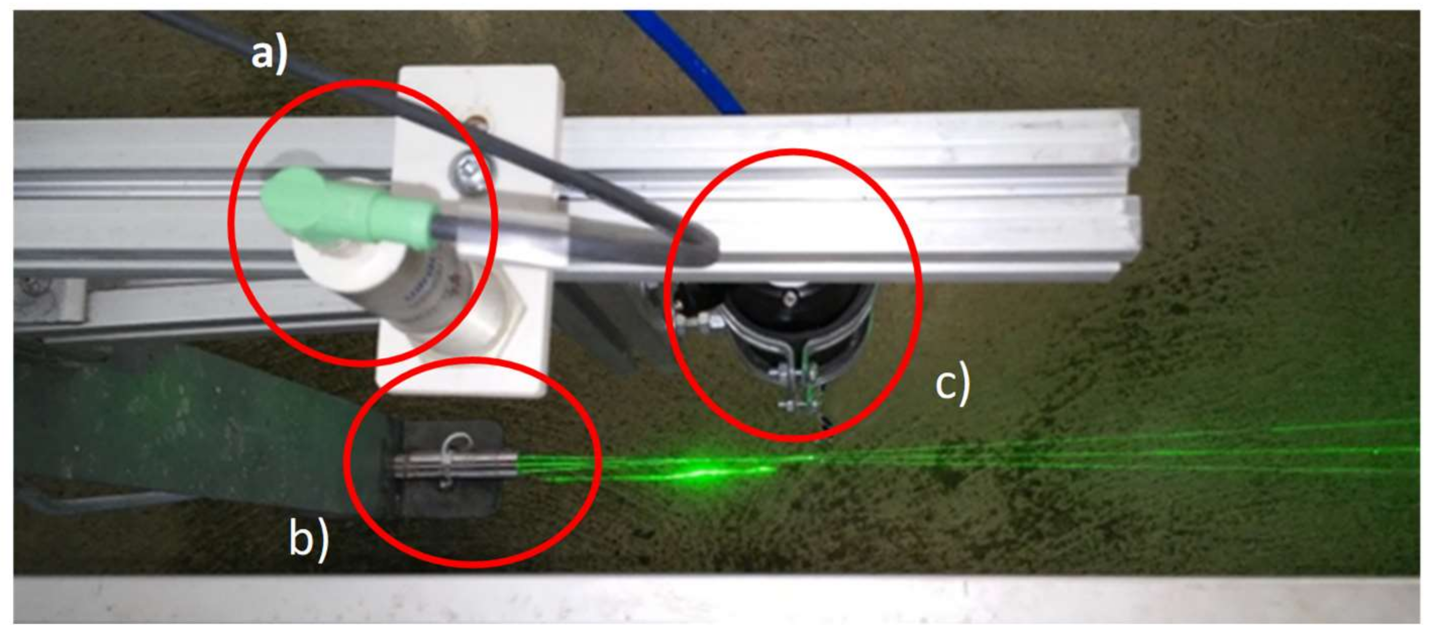
In view of the above, the main aim of our paper is to bring to the attention the cause-effect relation between surface convective deceleration and vorticity generation in plunging breakers. Such a goal is pursed by using both experimental and numerical means. First, Laser Doppler Anemometer (LDA) velocity measurements have been used to detect the time-averaged vorticity field in the pre-breaking region of a plunging breaker. Then, a calibration of the SPH model has been performed, by comparing experimental and numerical velocity and elevation time series obtained at different locations along the channel. Finally, SPH simulations have been used in the surf zone (i) to inspect and detail the vorticity field, evaluating, in particular, its temporal evolution; (ii) to relate the vorticity field and the free surface dynamics, in particular with the flow surface-parallel deceleration.

2. Experimental Set Up

Experimental investigations were carried out in a two-dimensional wave channel in the Coastal Engineering Laboratory (LIC) of the DICATECh of the Polytechnic University of Bari. The wave channel was 2.42 m wide and 45.20 m long. A uniform and fixed slope 1:10 started at 32.58 m from the paddles. The wave generating system is a piston-type one, with paddles producing the desired wave by providing a translation of the water mass, according to the proper input signal. Due to its dimension the channel can be considered a large-scale facility, with minimized scale effects. A picture and a sketch of the wave channel are shown in Figure 1 and Figure 2.

Table 1. Experimental parameters of the analysed regular wave.

Hs (cm)	TP (s)	L (m)	d (m)
10	2	5.10	0.80

shows the main characteristics of the tested regular wave near the paddles, i.e., wave height H_s, wave period T_p and wavelength L according to the Airy theory. The mean water depth was d. Considering the Irribarren breaking number ξ_b, the wave field is characterized by a plunging breaker (ξ_b = 0.71). The breaking section was located at a distance of 39.48 m from the wave paddle and the depth at breaking was around 11 cm.

Water surface elevations and velocities were measured at fourteen different locations along the centreline axis of the wave channel. Along each vertical profile, velocity measurements were acquired starting from the still water level. The measured points were 1 cm vertically spaced in the most superficial layer (for a thickness of 4 cm) and 0.5 cm vertically spaced in the remaining water column. The sketch of Figure 2 shows the four sections named 0, 1, 2, and 3, used in the present work for the SPH model calibration, and the pre-breaking region where further ten shoreward sections were investigated, being 1 cm longitudinally spaced (see

Table 2. Location of the measurements sections used for the code calibration and water depths.

Investigated Section	Distance from Paddles (m)	d (m)
Section 0	39.18	0.14
Section 1	39.08	0.15
Section 2	38.24	0.23
Section 3	37.04	0.35

). The cross-shore direction is given by the x axis and the vertical by the z axis.

Velocity measurements were performed at each vertical profile along almost the entire water column by means of a 2D LDA (by Dantec). Only for the bottom layer, where the LDA could not be used for technical limitations, an Acoustic Doppler Velocimetry system (ADV vertical looking Vectrino Velocimeter by Nortek) was adopted (Figure 3), characterized by an accuracy of 1 mm/s for the examined velocity range and a sampling frequency of 25 Hz. At the same time and location, water surface elevation was measured by an ultrasonic system UltraLab (by General Acoustics), with an accuracy of 2 mm. Data processing has included numerical filtering of wave elevation, despiking of ADV signal and filtering of the LDA acquisition based on a high signal to noise ratio.

3. SPH Numerical Method

SPH is a meshless, Lagrangian method where the fluid domain is represented by nodal points that are scattered in space with no grid structure and move with the fluid. A general description of the SPH can be found in [32,33,34]. The specific features of the SPH method here used are detailed in [26,35].

Vertically-2D simulations have been performed through a Weakly Compressible SPH (WCSPH) approach, in which an artificial compressibility is introduced to solve explicitly in time the equations of motion of an incompressible fluid. Monaghan [33] demonstrated that the error associated with the use of a compressible formulation for the incompressible free-surface water flow is bounded to 1%, provided the local numerical Mach number be everywhere lower than 0.1: here, this condition is ensured by means of an artificial speed of sound in water of 30 ms⁻¹. Such artificial speed of sound is not related to the physical speed of sound, which would be two orders of magnitude higher. It is introduced to avoid the extremely small time steps that would arise from the Courant stability condition, owing to the explicit scheme used for time integration. Monaghan [33] demonstrated that no unphysical compressibility effects arise if the local (numerical) Mach number, i.e., the ratio of the local velocity to the artificial speed of sound, is everywhere lower than 0.1. Numerical tests on flapping jets [31] have shown that this limit may be even stricter (0.05). Here, given that the highest velocities in the computational domain are lower than 1 m/s, a uniform value of 30 m/s was used for the artificial speed of sound, in order to guarantee a local Mach number smaller than 0.035.

The Reynolds-averaged Navier–Stokes (RANS) equations are implemented by an SPH semi-discrete form as:

$$\{\begin{array}{c}\langle \frac{\mathrm{D}{\rho }_i}{\mathrm{D}t}\rangle ={\displaystyle {\displaystyle \sum }_j}{m}_j\left({\mathit{v}}_i-{\mathit{v}}_{\mathit{j}}\right)·\widehat{\nabla }{W}_{ij}\\ \langle \frac{\mathrm{D}{\mathit{v}}_{\mathit{i}}}{\mathrm{D}t}\rangle =-{\displaystyle {\displaystyle \sum }_j}{m}_j\left(\frac{p_i}{{\rho }_i^2}+\frac{p_j}{{\rho }_j^2}\right)\nabla W_{ij}+{\displaystyle {\displaystyle \sum }_j}{m}_j\left({\mathcal{T}}_i-{\mathcal{T}}_j\right)·\widehat{\nabla }{W}_{ij}+g\\ \begin{array}{c}{p}_i-p_0=c_i^2\left({\varrho }_i-{\rho }_0\right)\\ {\mathcal{T}}_i={\mu }_{T_i}{\mathcal{S}}_i\end{array}\end{array}$$

(1)

where the angled brackets indicate the SPH particle approximation, written for each particle i having mass mi. Summation is extended to all particles j at a distance from i smaller than 2 h, i.e., lying within the circle where the C2 Wendland kernel function W_ij is defined [36].

In Equation (1), v = (u, v) is the velocity vector, $p$ is pressure, $\rho$ is density, $g$ is the gravity acceleration vector, $\mathcal{T}$ is the turbulent shear stress tensor, c is the speed of sound in the weakly compressible fluid, ${\mu }_T$ is the dynamic eddy viscosity, $\mathcal{S}$ is the rate-of-strain tensor and the subscript 0 denotes a reference state for pressure computation. All variables are assumed to be Reynolds averaged.

A standard k-ε turbulence model [37] has been used to obtain the eddy viscosity as ${\mu }_T=c_{\mu }\frac{k^2}{\epsilon }$: the equations for the turbulent kinetic energy k and for the turbulent dissipation rate ε in the SPH semi-discrete form [26,35] are:

$$\begin{gathered} \frac{D{k}_i}{Dt}=P_{k_i}+\frac{1}{{\sigma }_k}{{\displaystyle \sum }}_j{m}_j\frac{{\nu }_{T_i}+{\nu }_{T_j}}{{\rho }_i+{\rho }_j}\frac{k_i+k_j}{r_{ij}^2+0.01h^2}{\mathit{r}}_{ij}·\nabla {\widehat{W}}_{ij}-{\epsilon }_i \\ \frac{D{\epsilon }_i}{Dt}=C_{{\epsilon }_1}\frac{{\epsilon }_i}{k_i}{P}_{k_i}+\frac{1}{{\sigma }_{\epsilon }}{{\displaystyle \sum }}_j{m}_j\frac{{\nu }_{T_i}+{\nu }_{T_j}}{{\rho }_i+{\rho }_j}\frac{{\epsilon }_i+{\epsilon }_j}{r_{ij}^2+0.01h^2}{\mathit{r}}_{ij}·\nabla {\widehat{W}}_{ij}+C_{{\epsilon }_2}\frac{{\epsilon }_i}{k_i}{{\displaystyle \sum }}_j\frac{m_j}{{\rho }_j}{\epsilon }_j{\widehat{W}}_{ij} \end{gathered}$$

(2)

where P_k is the production of turbulent kinetic energy depending on the local rate of deformation and ν_T is the kinematic eddy viscosity. Like in [38], the values originally proposed by [37] for the model constants (σ_k = 1, σ_ε = 1.3, C_ε1 = 1.44, C_e2 = 1.92) have been maintained.

Notation $\widehat{\nabla }{W}_{ij}$ in Equations (1) and (2) indicates the gradient of W_ij, renormalized through a procedure which enforces consistency on the first derivatives to the 1st order [39], leading to a 2nd-order accurate discretization scheme in space. The kernel renormalization is applied everywhere, apart from the pressure gradient term, where the form originally proposed by [33] is retained to guarantee momentum conservation.

The semi-discrete system (Equations (1) and (2)) is integrated in time by a 2nd-order two-stage XSPH explicit algorithm [38], where each particle is moved according to a velocity

$${\mathit{v}}_i^X=\phi {\displaystyle \sum }_j\frac{m_j}{{\rho }_j}{\mathit{v}}_j{\widehat{W}}_{ij}+\left(1-\phi \right){\mathit{v}}_i^{n+1}$$

(3)

where $\phi$ is a velocity smoothing coefficient and v_iⁿ⁺¹ is the value obtained by solution of the second equation in (1).

A pressure smoothing procedure is also applied to the difference between the local and the hydrostatic pressure values [26] and contributes to reduce the numerical noise that affects the WCSPH owing to high frequency acoustic waves [40]. This approach proved to be effective in SPH analyses of different free-surface flows [35] and constitutes a valid alternative to other methods, such as δ-SPH [40], where a numerical diffusive term for density is added to the continuity equation, or filtering of the high-frequency pressure oscillations is used [41,42].

Finally, wall boundary conditions are imposed through the ghost particle method [43], i.e., by mirroring the positions of the inner SPH particles beyond the wall and by assigning to the latter the proper velocities and pressure conditions to obtain a Dirichlet condition for the velocity and a Neumann condition for the pressure.

4. Numerical Tests and Calibration of SPH Parameters

In this section the SPH model is employed to simulate the breaking wave on a sloping plane. See Table 1 for the experimental data.

The numerical domain was 22.5 m long and 1 m high, shorter than the laboratory channel. Such shorter domain was chosen to reduce the computational cost without influencing the quality of the numerical solution, as shown by [25,26].

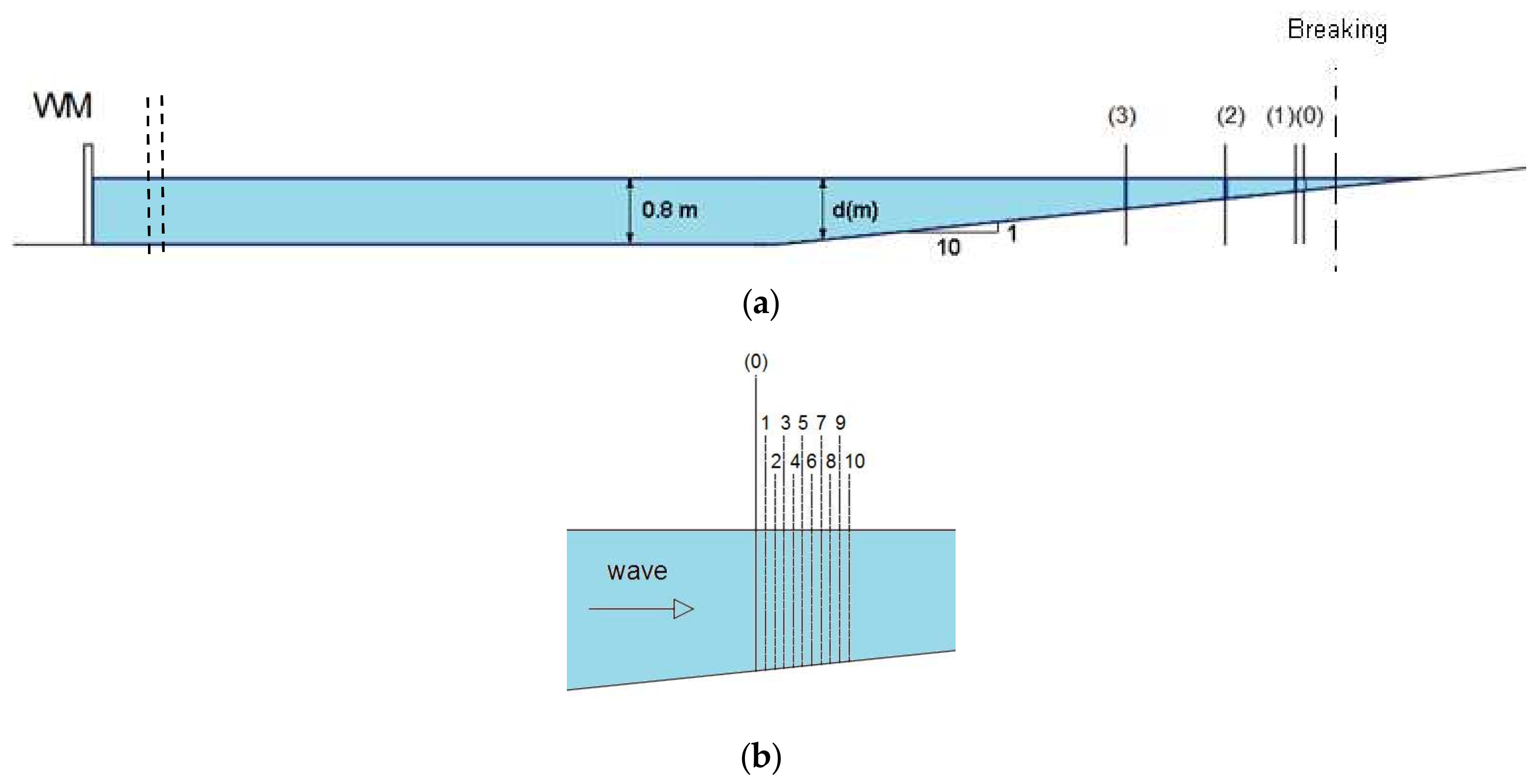
The offshore boundary condition has been modelled by a numerical wave paddle. i.e., by a moving-wall boundary condition imposed by ghost particles, whose motion has been forced to obtain the frequency and amplitude of the wave paddle needed to generate the desired sinusoidal wave. Section 0 is located at x = 14.6 m from the numerical wave paddle (thus the paddle is the origin of the x reference system, x = 0). The initial water depth is set equal to 0.80 m.

The choice of the initial particle spacing Σ depends on the physical process of the problem and on the desired computational accuracy and efficiency. The accuracy of particle methods is influenced by the initial particle spacing Σ, as well as by the smoothing length η. Both parameters must be taken into account when attempting to improve the resolution of the numerical simulation. It has been shown that the efficiency of the SPH kernel function depends also on the choice of the η/Σ ratio [44] and that a value η/Σ ≥1.2 should be preferred [45]. 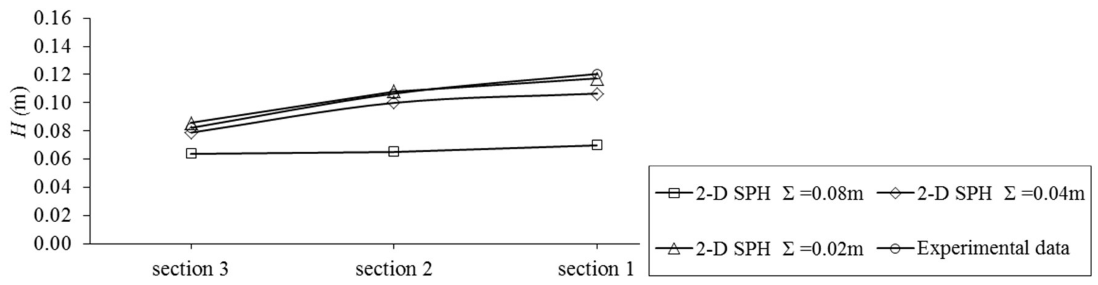Maintaining the value of η/Σ =1.5 constant, the effect of particle resolution on the quality of the numerical results has been investigated and a convergence analysis carried out (Figure 4). Simulations have been performed by choosing a coarse and a fine initial particle spacing (Σ); in particular, the 2D flow has been simulated by discretizing the computational domain through a value of particle spacing Σ varying from to 0.08 to 0.02 m.

The related number of SPH particles in the computational domain ranges from about 1500 to 24,000, respectively. The simulations have been performed with a velocity smoothing coefficient in the XSPH scheme $\phi$ equal to 0.02 (Equation (3)). Figure 4 shows the comparison between the numerical crest heights and the laboratory measurements at the chosen locations (Figure 2), by using the three different spatial resolutions reported above. The large spatial dimension of the SPH particles can also help explain the differences between the experimental data and the SPH results. In particular, Figure 4 shows the smoothing effect of a too low particle resolution (Σ = 0.08 m, N = 1500) on the description of the breaking wave. The simulation with the lowest resolution cannot adequately predict the experimental results. Figure 4 also shows that a value of particle spacing Σ equal to 0.02 m (N = 24,000) leads to a significant improvement of the simulated results in term of wave heights. Therefore, the reference SPH simulation was performed with particle spacing Σ equal to 0.02 m.

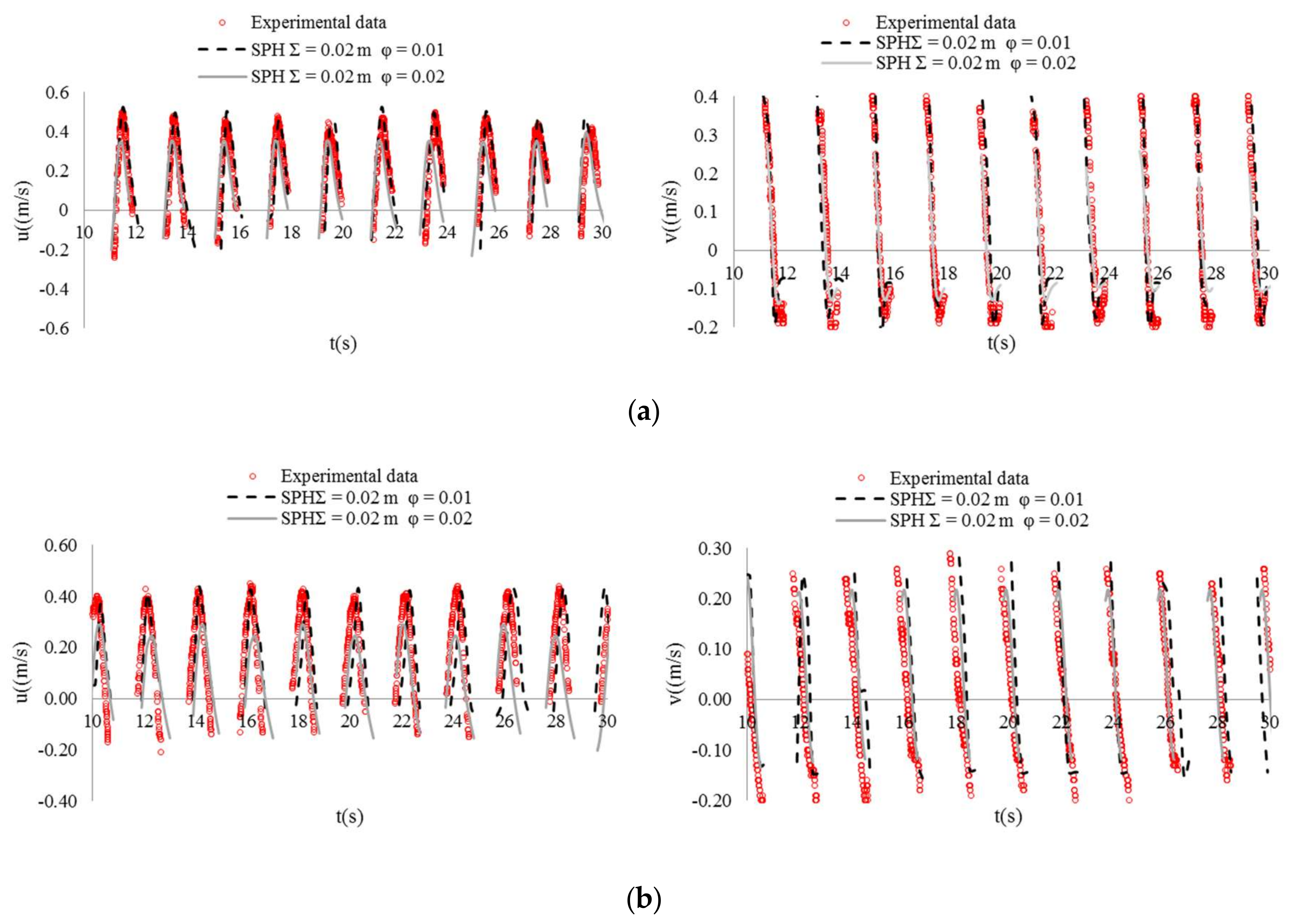
The effect of the velocity smoothing parameter has also been investigated. Simulations with an initial particle spacing Σ = 0.02 m have been run with two different $\phi$ values, equal to 0.01 and 0.02, respectively. While the computed values of crest height appear to be almost independent from $\phi$, the computed horizontal (u) and vertical (v) velocity components at the investigated sections (Figure 2) are underestimated when increasing the smoothing coefficient. With a very low value of the velocity smoothing parameter (φ < 0.01), the SPH method is unstable and one manifestation is that each of the particles begins to move chaotically for an excessive velocity. As an example, in Figure 5 both laboratory and numerical velocities at vertical Sections 2 and 3 are plotted, referring to the point located at 1 cm from the free surface. Therefore, the value $\phi$ = 0.01, which guarantees the stability of the SPH solutions without affecting the quality of the numerical results, has been chosen for the following runs.

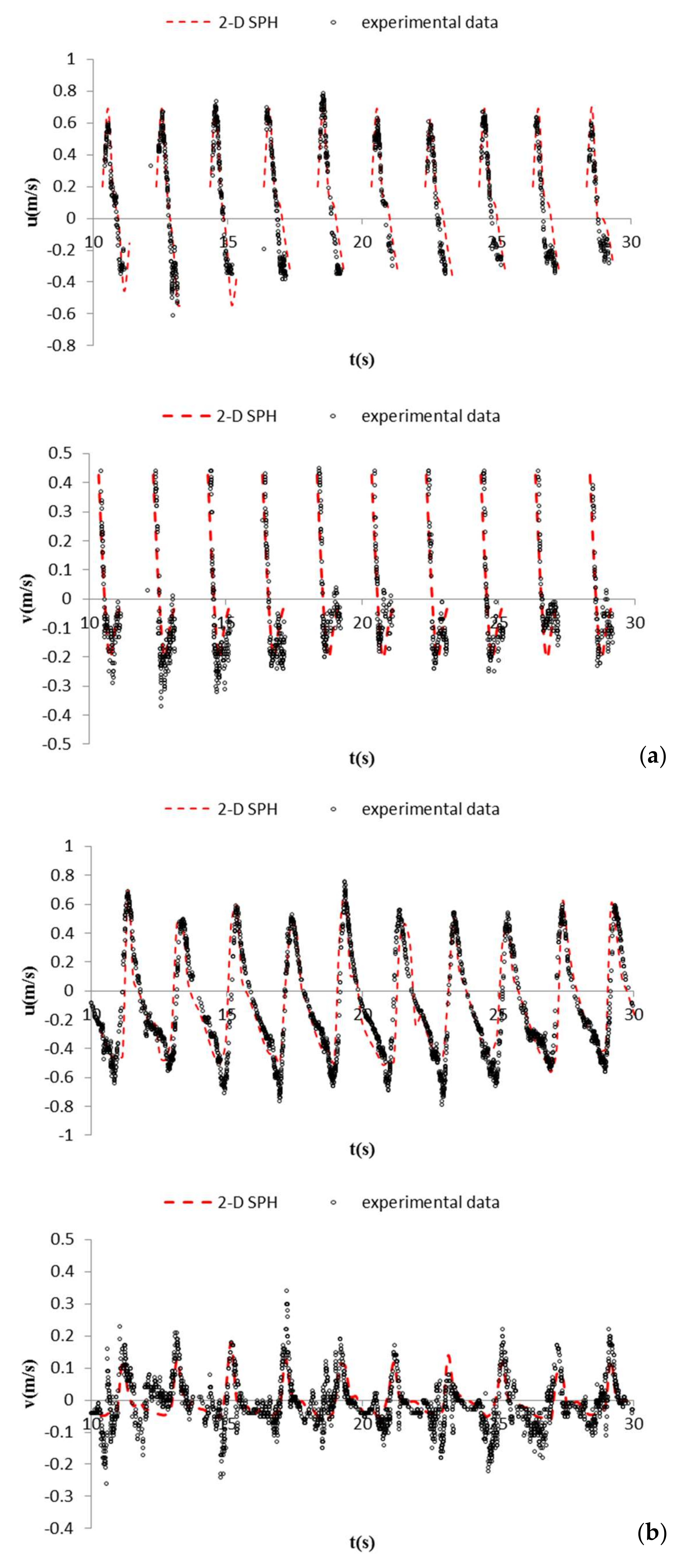
After this sensitivity analysis, the time series of the horizontal and vertical velocity components have been compared at Section 0 for all the investigated vertical locations. The agreement between the calibrated numerical results and the laboratory measurements is fairly good: Figure 6 illustrates a representative comparison, referring to both a superficial (Figure 6a) and a near-bed point (Figure 6b). Near the channel bed local effects (i.e., bed not perfectly smooth) could affect the vertical velocity component, this leading to a relatively poorer agreement (Figure 6b).

A global assessment of the model performances has been made by using the Wilmott index [46]:

$$I_w=1-\frac{{{\displaystyle \sum }}_{k=1}^N{\left(X_{C_k}-X_{m_k}\right)}^2}{{{\displaystyle \sum }}_{k=1}^N{\left[\left|X_{C_k}-\overline{X_m}\right|+\left|X_{m_k}-\overline{X_m}\right|\right]}^2}$$

(4)

a statistical parameter in which Xc and Xm are the modelled and measured values, respectively, while the bar denotes the average of the modelled and measured values. I_W takes a value of 1, when a perfect agreement exists between the measured and modelled values, while a value of I_W close to 0 denotes a complete discrepancy between numerical and experimental results. For the present run, all points placed along the vertical of Section 0 have been considered (sum for k between 1 and N), providing values of I_W equal to 0.95 and 0.90 for the horizontal and vertical velocity components, respectively.

5. Investigation on the Vorticity Generation

The characteristics of the vorticity characterizing the pre-breaking and breaking stages of the plunger have been studied both experimentally and numerically by means of the calibrated SPH numerical model. The vorticity is defined as

$$\omega =\left(\frac{\partial U}{\partial z}\right)-\left(\frac{\partial V}{\partial x}\right)$$

(5)

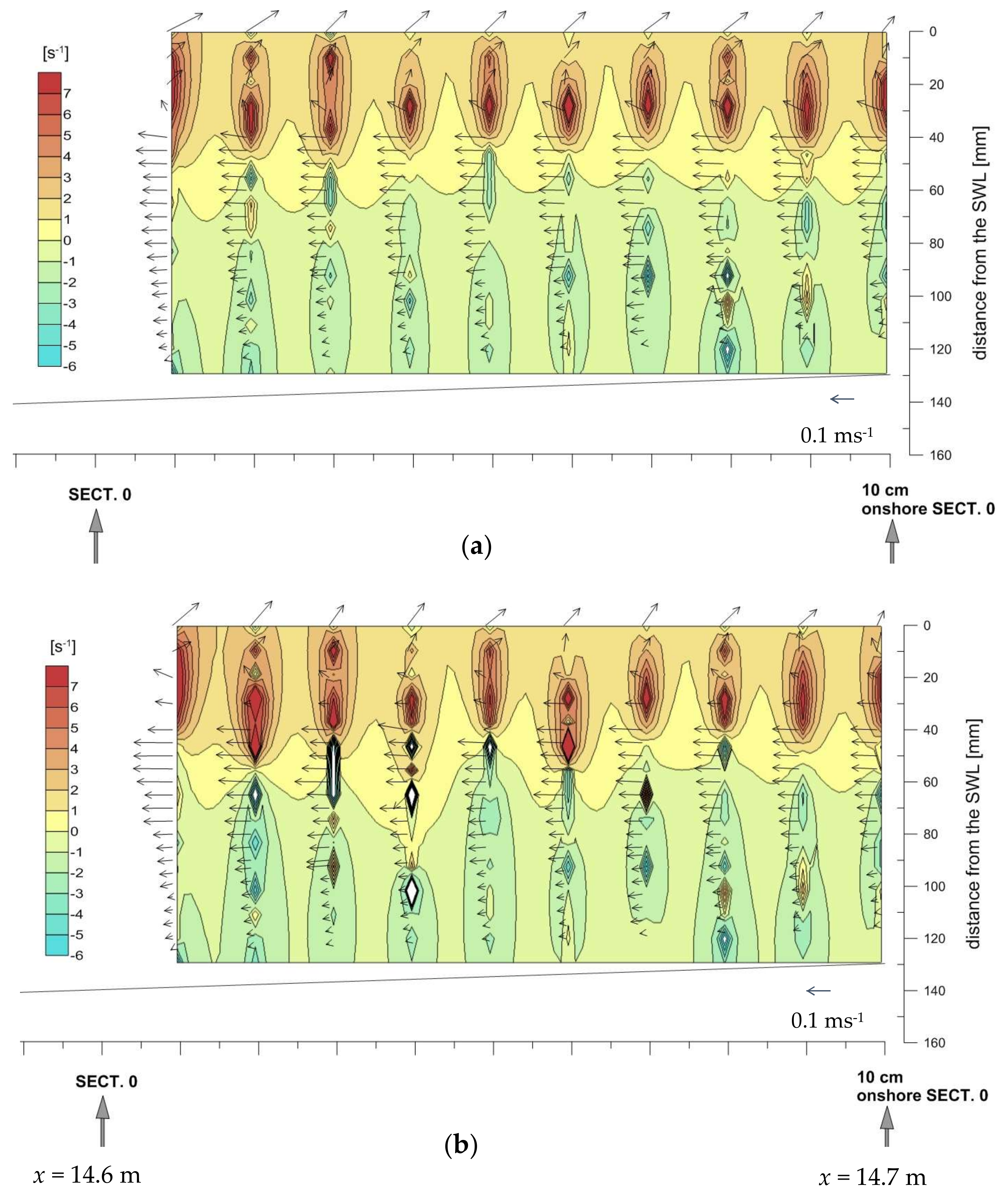
This has been computed using both the experimental data and the numerical output in the pre-breaking region of the plunging breaker, i.e., onshore Section 0 (Figure 2). U and V in Equation (5) are the time-averaged horizontal and vertical velocity components. Figure 7a,b displays the time-averaged velocity vectors superposed to the map of mean vorticity, respectively for the experimental data and the numerical solution.

Experimental values of vorticity have been evaluated for all the measured points (about 220 points). The averaging time for the experimental data is the whole acquisition period, i.e., about 80 s, and for the numerical data is 60 s. For a comparison in terms of time-averaging, this number of waves (i.e., ~40 and 30 for the experimental and numerical case, respectively) has been proved sufficient, a steady condition being reached. A very good match is observed between the experimental data and the numerical solution, both for the velocity profiles and for the vorticity field. The time-averaged velocities highlight the undertow structure (middle and lower part of the water column), while in the region above the wave through the flow displays a significant seaward drift, associated to the wave crest that is evolving to give a plunging jet.

Both experimental and numerical data show that most of the vorticity is due to the pre-breaking, free surface dynamics, with a much weaker contribution from the seabed shear. Figure 7a,b displays large positive (clockwise) vorticity over most of the upper water column, while, some smaller, negative (counterclockwise) vorticity characterizes the lower part of the water column, seaward of the breaking point, which approximately occurs at about 30 cm shoreward of Section 0 (Figure 2).

The positive vorticity of the upper water column has a background value in the range [0–3 Hz], while local maxima reach even 7 Hz. This is about the same order of magnitude of the wave phase speed divided by the local water depth, also found by [12] outside the aerated region. Negative background vorticity in the lower part of the water column is in the range [0–2 Hz] while local maxima are observed around −4 Hz. The cyclic pattern illustrated in Figure 7a,b (both upper and lower) is only due to the interpolation spacing used for plotting (equal to the spacing used in the computation of ω).

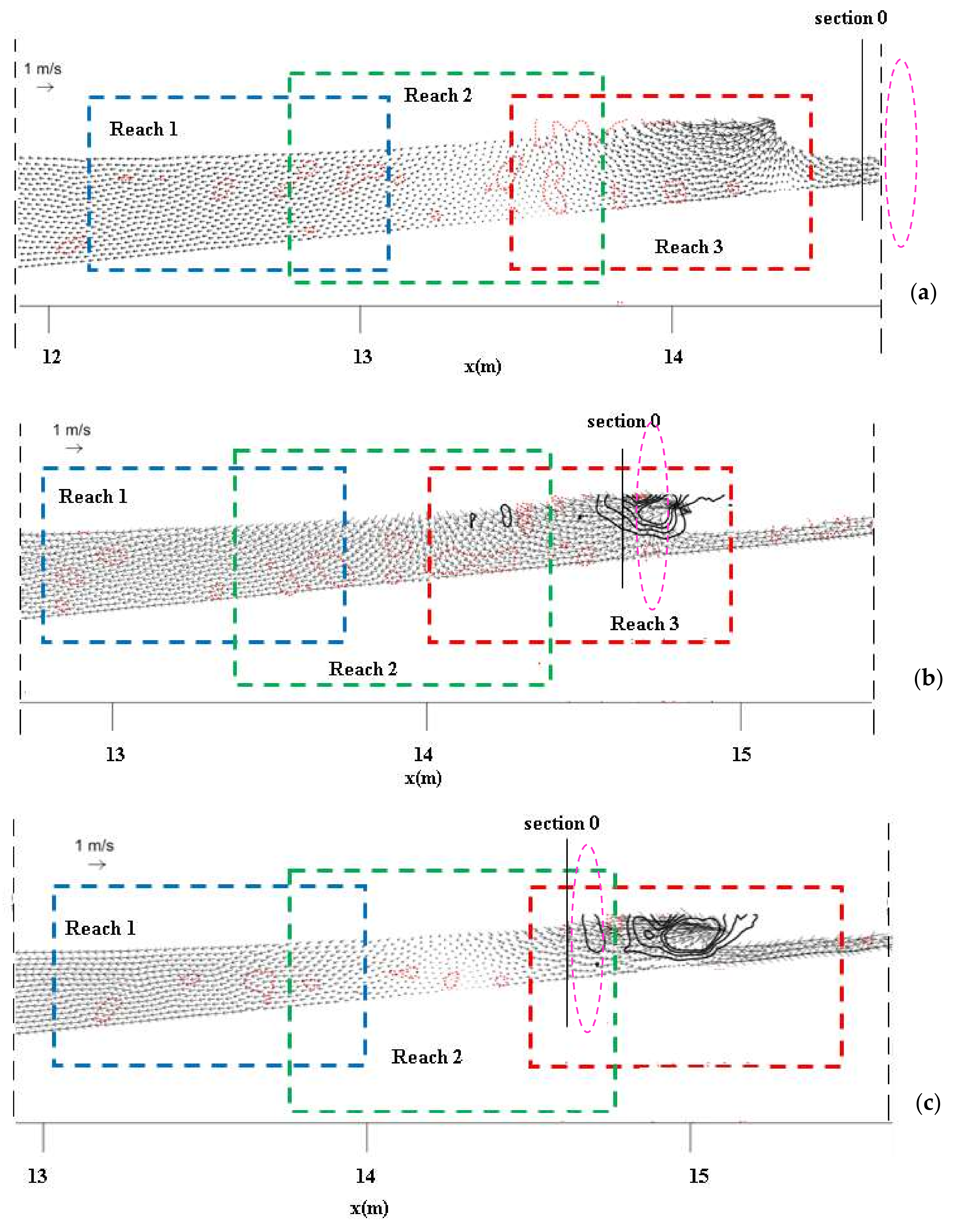
In order to better characterize the vorticity field, the numerical study has been focused to the time evolution of the vorticity field. Three reaches have been examined along the channel, as shown in Figure 8, and the numerical results are illustrated for three different times, i.e., before, during and after the breaking event. Specifically, we identify the breaking event as the impact of the plunging jet with the free surface. This also means that the conditions referenced as “before breaking” and “after breaking” occur T/4 before and T/10 after splash-down, respectively, as identified by inspecting the instants preceding and following the impact of the jet on the surface. Therefore, the “after breaking” condition displays features due to the jet impact. The three analysed reaches partly overlap and move following the wave. In this numerical case, the vorticity is computed using instant values of the horizontal and vertical velocity in Equation (5). Vorticity contour lines—black giving positive and red giving negative vorticity, respectively—are superposed to the velocity vectors, giving size and direction of the velocity field (Figure 8a–c).

Figure 8a highlights that before breaking very low negative vorticity is locally present in all the three reaches, especially near the bottom in reach 3, and spreads towards the surface in reach 2 and 1. Since the previous wave has just moved along the same reaches, with a fast-moving crest and the opposing slower-moving water below the trough, these negative values still present in the channel should be regarded as the residual effect of the previous wave. During breaking (Figure 8b), due to the impact of the jet on the surface, flow separation occurs and positive vorticity is generated and propagates with the uprush flow, while negative vorticity forms in the downwash flow and slowly spreads in the return flow along the channel. After breaking (Figure 8c), positive vorticity persists near the surface in reaches 2 and 3, while negative vorticity rapidly decreases.

We analysed this vorticity generation in the light of flow separation at the free surface (see, as reference, the case of flow separation at a hydraulic jump illustrated by [47], i.e., in the light of fluid deceleration). Hence, we regard the analysis of fluid deceleration at a spilling breaker by [21] as a useful reference for our analysis. Dabiri and Gharib [21], verified that the vorticity was also convected due to the sharp velocity gradient of the fluid near the free surface with respect to the fluid below. To better explore this aspect, we also computed the surface parallel convective acceleration, U_s ∂U_s/∂s which also represents a fundamental contribution to the flux of near-surface vorticity as shown by Equation (8) of [21].

In fact, Dabiri and Gharib [21] demonstrate that the dominant terms in the vorticity flux of surface-parallel vorticity through the surface are the gravity and the deceleration terms.

Assuming that the gravity term remains constant, Dabiri and Gharib [21] theoretically derived that near-surface vorticity increases with increasing deceleration term.

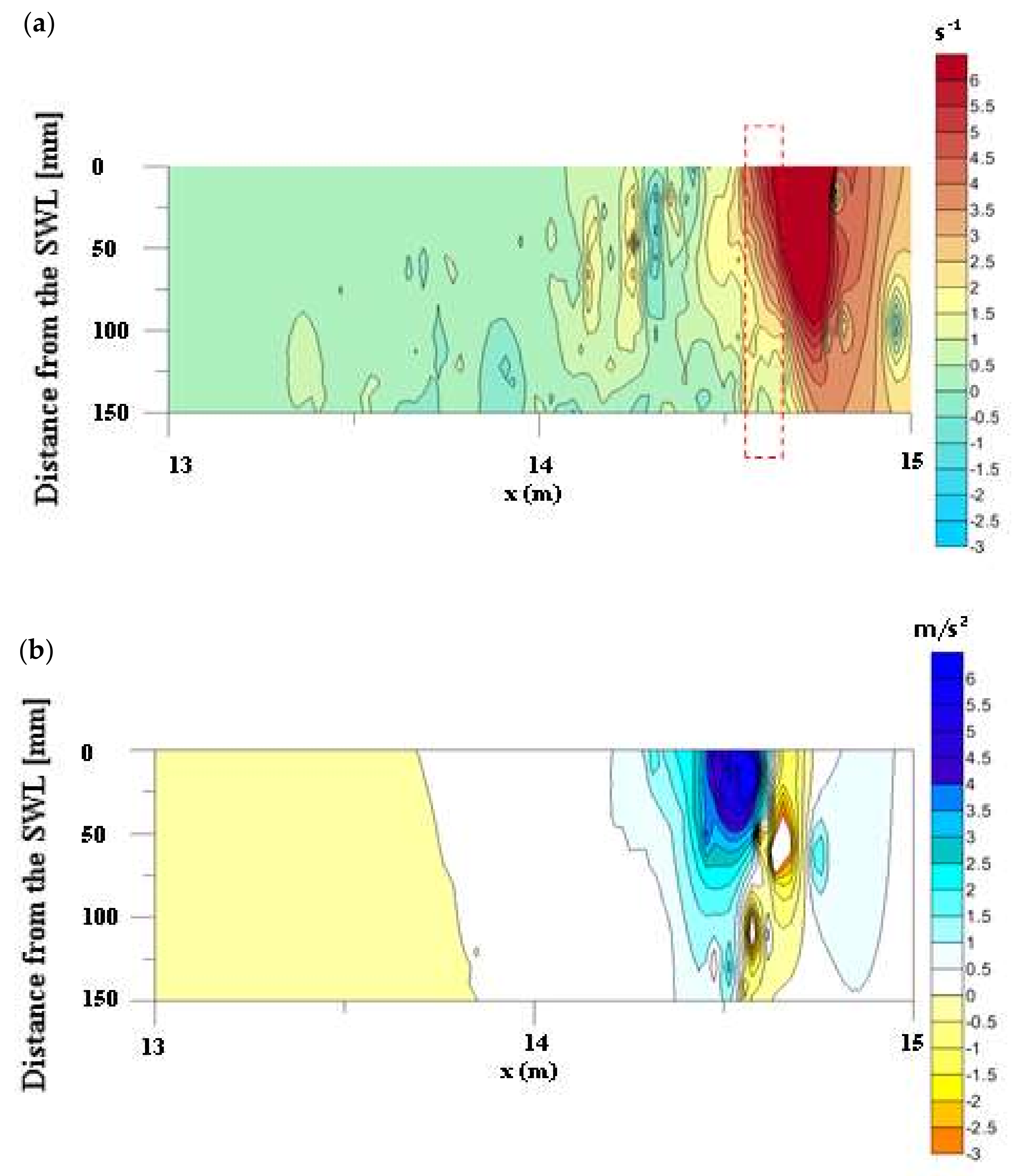
Figure 9 show the comparison between the instantaneous map of vorticity and of the surface parallel convective acceleration, along reach 3 and for the upper half of the channel. The flow acceleration due to the convective term U_s ∂U_s/∂s has been computed taking as s a curvilinear coordinate running to the free-surface, so that it is accurate near the mean surface where the streamlines closely follow the surface. As shown by [47], the mean surface-parallel velocities were calculated as:

$$U_s=U\cos \theta -V\sin \theta$$

(6)

where θ is the angle that the tangent to the mean surface makes with the horizontal axis.

A flow deceleration occurs in the same location where peaks of positive vorticity appear. Referring to reach 3 during the breaking event, the vorticity reaches its maximum near the surface where the wave plunges (Figure 9a) and where also the surface-parallel convective deceleration, or vorticity flux (see [47]) strongly increases (Figure 9b). This vorticity does not decay rapidly away from the mean surface. Rather, the flow remains rotational along the whole depth.

For a direct, though qualitative, comparison with Figure 7, the marked box in Figure 9a delimits the corresponding experimental and numerical areas.

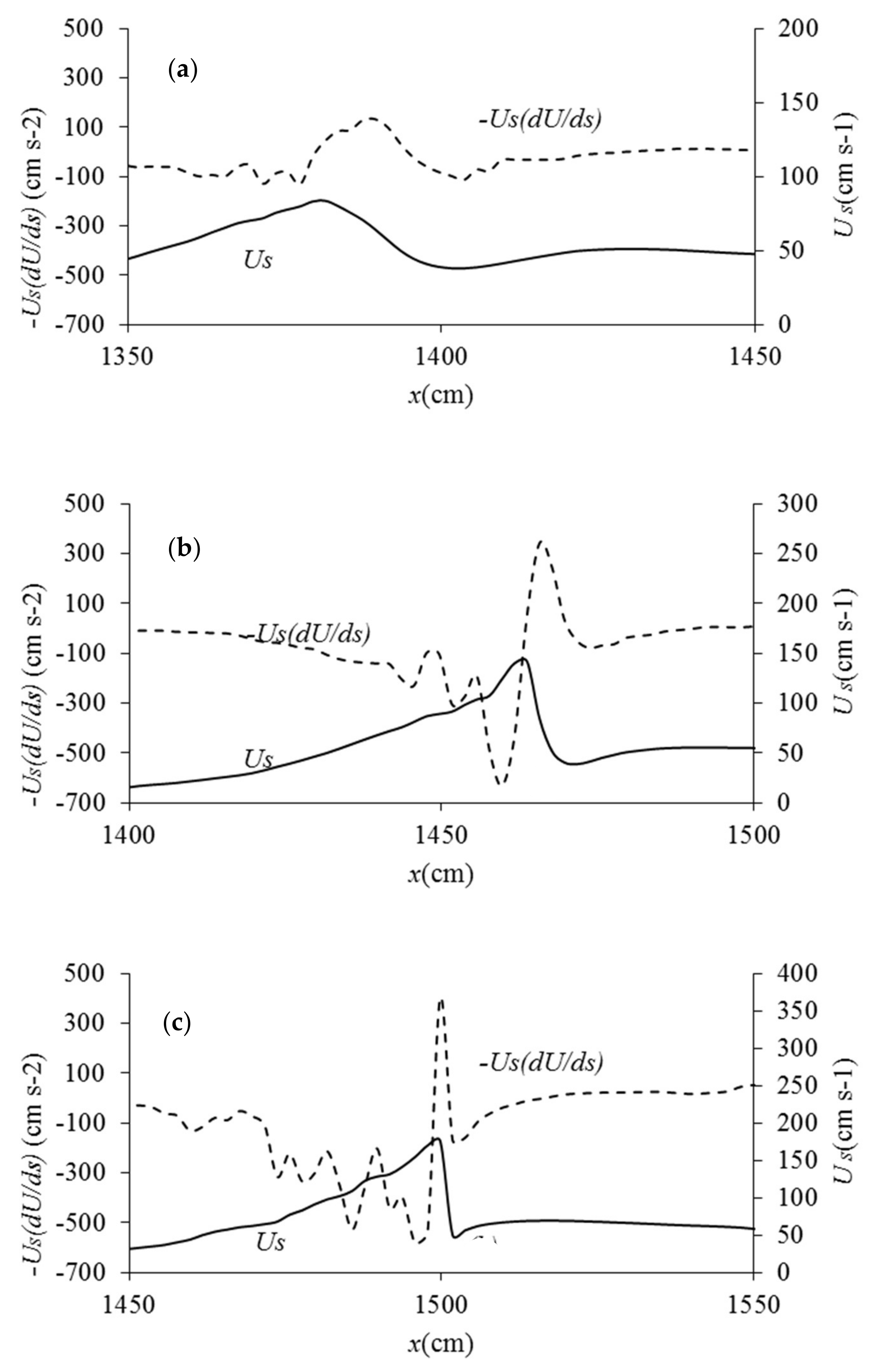
In more detail, Figure 10 shows both the numerically-computed, surface-parallel deceleration term and the surface velocity U_s along reach 3, at the points nearest to the free surface, respectively before, during and after breaking. Trends observed in the spatial maps of Figure 9 are confirmed.

The deceleration term and the surface velocity along reach 3 before breaking (Figure 10a) do not display any evident peak, meaning that at this stage and location there is no significant flux of vorticity. This is consistent with the map of Figure 8a, where in reach 3 no new positive vorticity is generated. During breaking (Figure 10b), the deceleration term is characterized by a peak at x = 14.6 m. It is preceded by a peak in the streamwise velocity (x = 14.57 m), while the minimum streamwise velocity is downstream, at x = 14.7 m. In other words, at the location of the maximum flow deceleration a large amount of vorticity is injected. Breaking is detected around x = 14.9 m. In Figure 10c, the peaks of the streamwise velocity and of the deceleration term are very close, being the first at x = 14.98 m and the second at x = 15 m. The minimum value of U_s is at x = 15.07 m.

The jet has moved onshore reaching its extreme evolution, with maximum velocity and vorticity, then rapidly impacts the free surface, inducing a flow reversal in the underlying water column. Again, the largest deceleration coincides with the peak of vorticity flux, suggesting that this behaviour is robust.

Both during and after breaking the streamwise velocity sharply decreases downstream the location where the deceleration peaks are observed. Nevertheless, contrarily to what observed by [21] for a spilling breaker, our findings do not show stagnation points for the streamwise velocity. The positive vorticity already observed in Figure 8b,c is located beneath the surface and concentrated at the same coordinates of maximum deceleration.

Similarly, to the case of a spilling breaker [21] and hydraulic jump [47], a cause-effect relation between near-surface flow deceleration and vorticity flux is thus experimentally proved also for the plunging case, this being a novel result with respect to previous studies. Once clarified this analogy with the spilling case, we also note some differences.

In particular, Dabiri and Gharib [21] observed an important surface-parallel flow deceleration at the toe of the spiller but excluded that the sharp curvature of the free surface could be the main cause of wave breaking, while Misra et al. [47] correlated vorticity generation with sharp free surface curvature changes and surface-parallel adverse pressure gradients. For the present plunging breaker, surface-parallel convective deceleration is observed at the wave crest bulge, with maximum immediately downstream of the sharp crest velocity reduction. Therefore, our findings, with some similarity to [47], lead us to think that a strong free surface deformation associated with near-surface flow deceleration induces an important generation of vorticity in the near surface flow, and leads to the plunger splash-down.

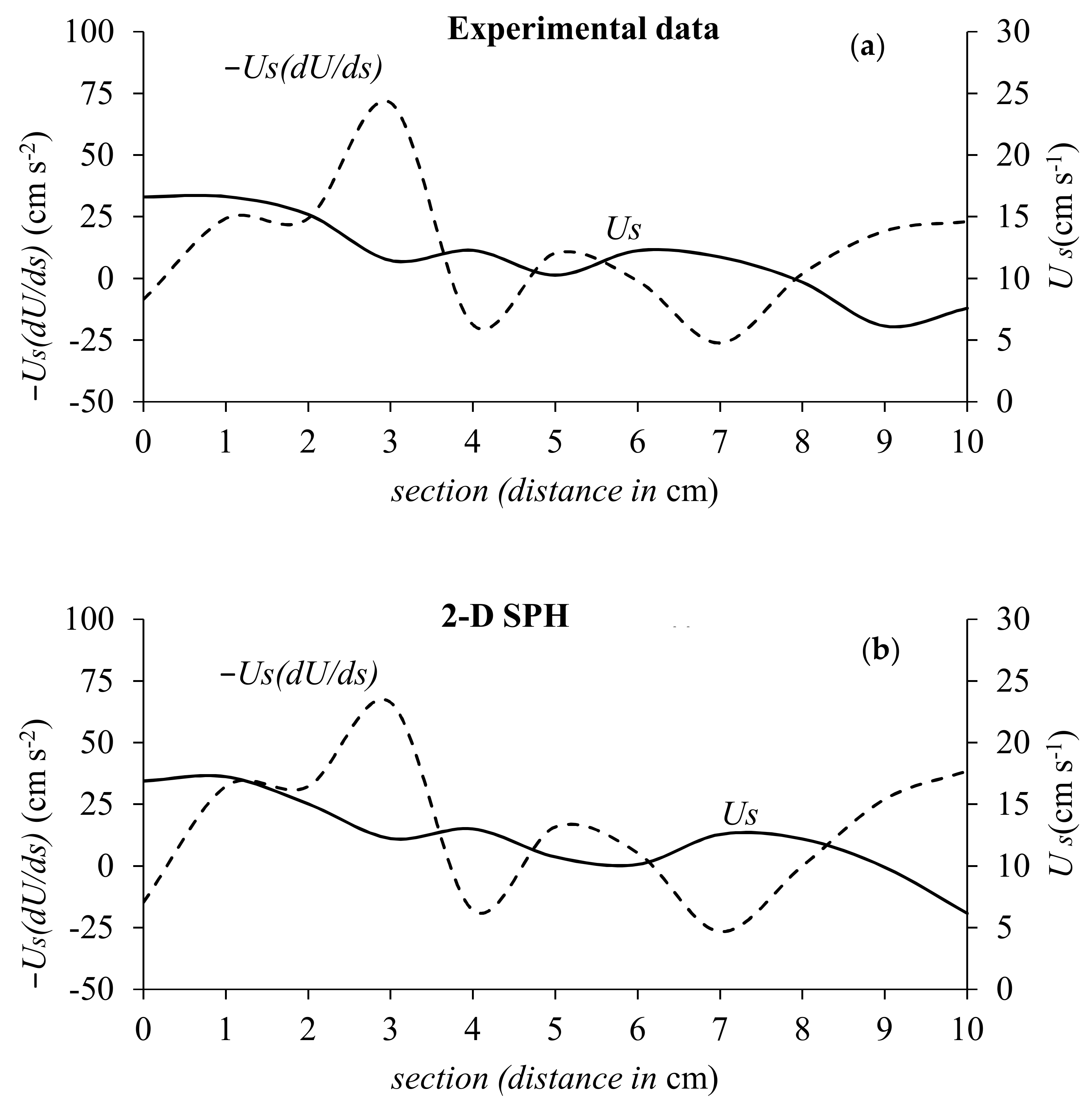
The deceleration term and the surface velocity were examined also for the experimental and numerical data, referring to time-averaged quantities (Figure 11) acquired onshore of Section 0, to confirm the interpretation of the mean flow vortical dynamics shown above. In a time-averaged sense, Figure 11a,b shows a peak of the deceleration term located 3 cm onshore of Section 0. Even this observation is consistent with the higher positive near-surface vorticity assessed and plotted in Figure 7a,b, thus confirming what numerically obtained.

These results can be of interest for different stakeholders because vorticity generation and spreading produce effects on the: (i) evolution of bed topography, as a result of a complex interaction between flow and sediment particles along the bed, being wave-breaking turbulence responsible for most of the sediment suspension through breaking injected eddies; (ii) air-water mixing, this being fundamental for ocean-atmosphere exchanges; (iii) mixing and transport of solutes, these being fundamental for water quality management purposes. Finally, information on the link between vorticity generations and turbulence spreading is also useful for numerical modeling, enabling improved calculations of water mixing over the entire water column and possibly limiting the computational efforts.

6. Conclusions

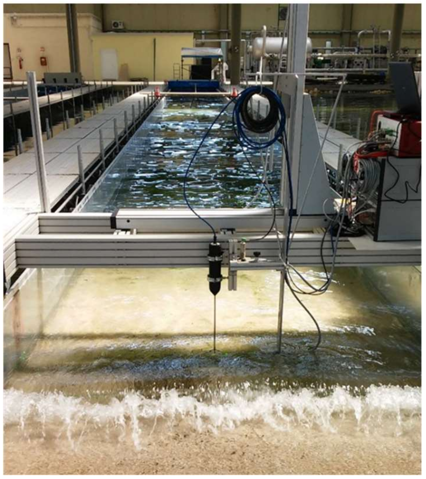
Vorticity generation in the pre-breaking and breaking zone of a plunger was examined in this study. Experimental measurements of fluid velocities, carried out in the wave channel of the LIC laboratory of the Polytechnic University of Bari, highlighted the presence of positive vorticity beneath the surface of the breaking wave. On the contrary negative vorticity was localized near the flume bed. This observation was the result of a time-average operation on velocity data assessed by single point measurement techniques, i.e., LDA and ADV.

To thoroughly investigate the vorticity field under the breaker and its temporal evolution, a numerical model was used. Specifically, a Weakly-Compressible SPH (WCSPH) scheme, which includes a two-equation k-ε turbulence model, was applied. Preliminarily, the SPH model was validated by means of both elevation and velocity laboratory data, providing a successful agreement between numerical results and measurements.

Then, the validated SPH model run to detail the vorticity field under the plunging breaker and to shed some light on the vorticity source. Three frames along the channel were examined, during three different instant times, i.e., before, during and after breaking. Numerical vorticity maps clearly show that new positive vorticity is generated beneath the free surface during and after breaking. The comparison between time-averaged experimental and numerical vorticity provided an excellent overall similarity.

Successively, starting from the instantaneous numerical streamwise velocity, the surface-parallel convective acceleration was computed, considering that it is a fundamental contribution to the flux of near-surface vorticity [21,47]. Its analysis shows that a flow deceleration occurs in the same locations where peaks of positive vorticity appear. This result is furtherly confirmed by the investigation of the surface-parallel deceleration in the points nearest to the free surface, respectively before, during and after breaking. Also, in this case, both during and after breaking, the largest deceleration coincides with the peak of vorticity flux, suggesting that this behaviour is robust. The novelty of our study is the detection for the plunging breaker of a cause-effect relation between near-surface flow deceleration and vorticity flux, similarly to the case of a spilling breaker [21] and a hydraulic jump [47].

However, differently from [21], our findings do not show stagnation points for the streamwise velocity. Moreover, in the present plunging breaker, the surface-parallel convective deceleration is observed at the wave crest bulge. With some similarity with the deductions by [47], this specific result lead us to think that both strong free surface deformation and near-surface flow deceleration induce an important generation of vorticity in the near surface flow, and lead to the plunger splash-down.

Analysis is underway to quantitative detail the relation between near-surface flow deceleration and vorticity injection into a plunger, with reference to what typically observed in spillers.