Wave Height Attenuation and Flow Resistance Due to Emergent or Near-Emergent Vegetation


1
Department of Civil, Architectural and Environmental Engineering, University of Padua, Via Loredan, 20, 35131 Padova PD, Italy
2
Department of Civil, Environmental, Land, Building Engineering and Chemistry, Polytechnic University of Bari, Via Edoardo Orabona, 4, 70126 Bari BA, Italy
*
Author to whom correspondence should be addressed.
Water 2018, 10(4), 402; https://doi.org/10.3390/w10040402
Submission received: 12 February 2018
/
Revised: 21 March 2018
/
Accepted: 27 March 2018
/
Published: 29 March 2018
(This article belongs to the Special Issue Turbulence in River and Maritime Hydraulics)
Abstract
:Vegetation plays a pivotal role in fluvial and coastal flows, affecting their structure and turbulence, thus having a strong impact on the processes of transport and diffusion of nutrients and sediments, as well as on ecosystems and habitats. In the present experimental study, the attenuation of regular waves propagating in a channel through flexible vegetation is investigated. Specifically, artificial plants mimicking Spartina maritima are considered. Different plant densities and arrangements are tested, as well as different submergence ratios. Measurements of wave characteristics by six wave gauges, distributed all along the vegetated stretch, allow us to estimate the wave energy dissipation. The flow resistance opposed by vegetation is inferred by considering that drag and dissipation coefficients are strictly related. The submergence ratio and the stem density, rather than the wave characteristics, affect the drag coefficient the most. A comparison with the results obtained in the case when the same vegetation is placed in a uniform flow is also shown. It confirms that the drag coefficient for the canopy is lower than for an isolated cylinder, even if the reduction is not affected by the stem density, underlining that flow unsteadiness might be crucial in the process of dissipation.
1. Introduction
Coastal wetlands and saltmarshes are fundamental for sustaining ecosystems and preserving coasts from erosion and flooding due to storm surge and waves [1,2,3]. In the last century a widespread reduction in these areas has been observed in countries where short-sighted human activities and an increase of the sea level have strongly affected the morphodynamic equilibrium of intertidal environments [4,5]. Since that vegetation plays a fundamental role in the preservation and restoration of this habitat by controlling the coastal hydrodynamics, an effective strategy to counteract this trend is to promote the development of alophyte plants in wetlands. In particular, vegetation attenuates the action of waves, slows down the flow, and promotes diffusion and deposition processes [6,7,8,9,10]. Accordingly, it (i) enhances particle removal and water quality [11,12,13]; (ii) positively affects the hydrochory and nautochory of seeds and organic matter [14,15,16,17]; (iii) reduces sediment erosion and resuspension, while enhancing sediment deposition [18,19,20]; and (iv) creates preferred paths for tracers’ dissipation processes [21,22,23].
This is one of the main reasons for investigations of the interaction between vegetation and flow. Wave attenuation has been widely investigated in controlled laboratory experiments, where vegetation has often been mimicked by rigid dowels or artificial plants [24,25,26,27,28,29], as well as in field observations, where it has been limited to cross-shore transects. [30,31,32,33]. Despite the large amounts of theoretical and experimental results available in the literature, the interaction of waves with a vegetated canopy still deserves further study. In particular, the drag coefficient, which represents/includes the impact of several phenomena such as sheltering, bed interaction, and non-uniform velocity distribution [34], needs to be assessed.
Wave attenuation resulting from wave–vegetation interaction depends on hydrodynamic conditions such as the incident wave height and period, and water depth, as well as on plant properties such as impact area, density, and flexibility. Many studies focused on different species of plants commonly diffused on saltmarshes and along coastal environments, in order to quantify the plant-specific attenuation of the waves, e.g., Laminaria hyberborea, Spartina alternifora, and Macrocystis pyrifera [35,36,37]. Although Spartina maritima is a common grass in wetlands and saltmarshes [38,39], only a few experimental studies have considered this type of vegetation [40].
The present work describes and discusses the results of an experimental investigation aimed at studying the flow resistance and wave attenuation capability of Spartina maritima. Experiments are carried out in the laboratory under controlled wave conditions; plastic plants mimicking Spartina maritima are arranged on the bottom of the wave-flume and experiments consider either emergent or submerged canopy, as well as different plant density. In order to compare and relate resistance characteristics induced by vegetation (e.g., the drag coefficient) under wave and steady flow conditions, additional experiments are performed in steady flow conditions using the same plastic plants, with varying density.
2. Materials and Methods
2.1. Experimental Setup
To investigate the wave attenuation induced by Spartina maritima, experiments are carried out in a wave flume 35.0 m long, 1.0 m wide, and 1.3 m deep; an HR Wallingford paddle generates monochromatic waves. At the opposite end of the flume, a wave absorber damps incident waves (see Figure 1). The wave absorber is made of a sloping (1:3) porous metal plate, covered with a needle-punched geogrid, which ensures, in the present experiments, a reflection coefficient smaller than 10%.
Fifteen meters downstream of the wave generator, a 16 m long false plane bottom houses the vegetation canopy; the 4 m long reach occupied by vegetation starts 8 m downstream from the upstream edge of the false plane. The artificial plants are inserted in adjacent PVC panels, which are drilled in order to fix the main stem of the plant into holes that are equally spaced 4 cm apart both longitudinally and transversally (see Figure 2a).
The artificial plants chosen for mimicking the real Spartina maritima are the same used in other studies aimed at investigating the transport and diffusion of floating seeds in partially emerged saltmarsh vegetation [41,42]. They are plastic plants 15 cm high, with ns = 120 stems having a diameter, , of approximately 2.0 mm. Real Spartina is compared to the present artificial plants in Figure 2b.
Six wave gauges measure the free surface oscillation in the flume at 20 Hz sampling rate. Five probes are placed at 0.00 m, 0.66 m, 1.32 m, 2.66 m and 4.00 m from the beginning of the vegetated area, and they recorded the wave attenuation along the canopy, whilst the sixth probe, located 1.5 m upstream of the vegetation field, recorded the approaching wave height, (see Figure 1).
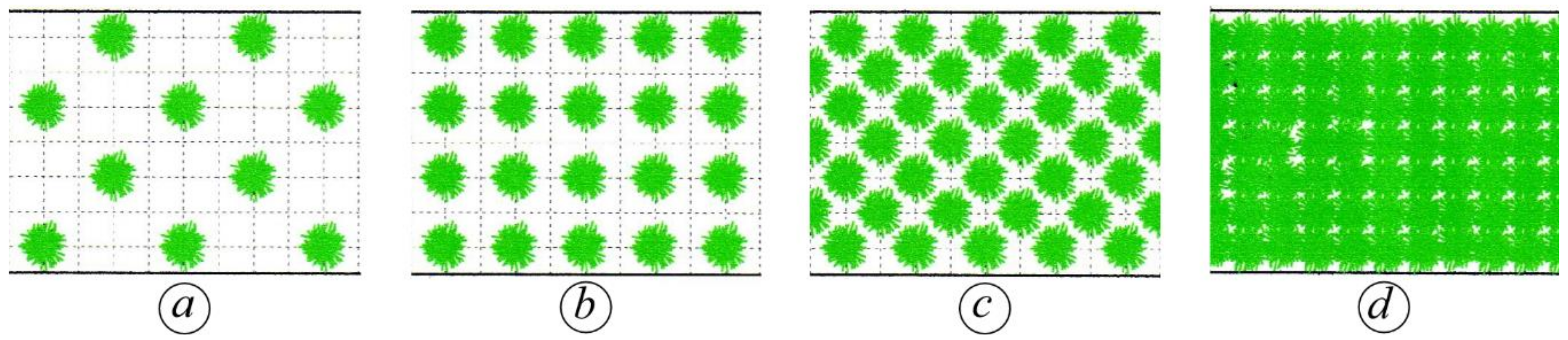
Two series of tests are performed. In the first series, waves attenuation is recorded considering four scenarios characterized by different plant configurations with densities = 43.75, 84.5, 156.25 and 312.5 plant/m2, arranged as in Figure 3. For each plant configuration, experiments are performed at five water depths, namely = 10, 15, 20, 25, and 30 cm. The wave period, , ranges between 0.7 and 1.4 s and the wave height, , is selected so that the slope (with the wave length) ranges between 0.01 and 0.09. The hydrodynamic conditions are summarized in Table 1.
In the second series of experiments, the configuration having the greatest vegetation density, i.e., = 312.5 plant/m2 is investigated in depth. For each of the water depths listed above, nine wave conditions, resulting from the combination of 3 wave periods, = 0.8, 1.0 and 1.2 s, and three wave slopes, = 0.03, 0.05 and 0.08, are investigated (for details see Table 1).
In order to compare and relate resistance characteristics induced by vegetation under wave and in steady flow conditions, additional experiments are performed in uniform flow condition (UF experiment). These tests are carried out in a 6.0 m long, 0.3 m wide, and 0.5 m high tilting flume, in which the same plastic plants are arranged over a 3 m long reach. To ensure uniform flow conditions, a magnetic flowmeter accurately measures the bulk flow rate, and constant water depth is achieved by adjusting the bottom slope and a downstream weir.
Four different plant arrangements are investigated, with equal to 78.125, 156.25, 312.5, and 625 plant/m2, respectively (see Figure 4). The bulk flow velocity is approximately 6.7 cm/s in all experiments, whereas, for each plant density, three water depths are considered, i.e., = 5cm, 10 cm, and 15 cm (Table 2). This means that the UF experiment investigate the behavior of flexible emergent vegetation ().
2.2. The Theoretical Model
The energy of waves propagating through and over vegetation is dissipated due to the action of waves on vegetation [24,26,27]. The general form of the energy conservation equation is
where is the wave energy, is the wave group velocity and is the time-averaged rate of energy dissipation per unit length induced by vegetation.
On assuming to be constant and recalling that , with the water density, the gravity, and the wave height, the above equation can be rewritten as
The dissipation rate is commonly estimated assuming the linear wave theory [6,26,29]. Mendez and Losada [26] obtained the following expression for :
where is the drag coefficient of the single stem, is the submerged stem height that is equal to in submerged condition (i.e., 1), and to in emergent conditions (i.e., 1), and is the average stems density, i.e., number of stems per unit area, is the wave number, and is the angular frequency.
In the present experiments all the parameters of Equation (3) are assumed to be constant, hence Equation (2) has the following analytical solution:
where is the incident wave height at , corresponding to the upstream cross section of the vegetated reach, and is the dissipation coefficient due to the vegetation
Alternatively, Kobayashi et al. [6] proposed to linearize the energy equation by approximating in Equation (3). With this assumption, the wave height decreases exponentially, as follows:
Both hyperbolic and exponential models, expressed by Equations (4) and (6) respectively, are commonly adopted in the literature to describe the wave attenuation in the presence of vegetation. Nevertheless, the results of the present investigations clearly show that the linearized solution fits the experimental results better.
The drag coefficient, , is the only unknown of the problem, hence it can be inferred from experimental data. Specifically, in the present experiments, is estimated by minimizing the difference between observed and expected wave attenuation according to Equation (6), Then, is estimated from Equation (5).
In the literature, the drag coefficient is expressed as a function of either the Reynolds number, , or the Keulegan–Carpenter number, . The stem Reynolds number is
where is the water kinematic viscosity and is the horizontal velocity amplitude averaged over the stem height, which can be approximated by the velocity at the top of the canopy, when is relatively small, i.e.,
is representative of the velocity magnitude acting on the stem, notwithstanding it is approximately the actual velocity at the top of the canopy, since the vertical velocity profile with submerged vegetation can differ quite a bit from the profile predicted by the linear wave theory [43].
The Keulegan–Carpenter number, also called the period number, is:
Most experimental studies express the drag coefficient as a power law of either or :
where and are calibration coefficients.
In the case of vegetated uniform flow, the literature provides many bulk expressions to estimate the drag coefficient, which are based on experimental, theoretical, and computational investigations [25,44,45,46].
Among the many available models, the simple model created by Nepf [25] for the case of a dense array of emergent rigid cylinders provides reasonable and effective results [46,47]. Therefore, this approach is used in the present study for the estimation of in the uniform flow experiments. The force balance in the flow direction is
where is the bed shear stress and is the flow velocity averaged over the stem height. In the present case, the stem density is very high and drag resistance turns out to be much greater than bed shear stress; accordingly, is neglected in Equation (11). In addition, only the emergent vegetation condition is investigated, so that is the bulk flow velocity. The choice to perform the UF experiment with only emergent vegetation is essentially due to the large variability of flow velocity in the vertical direction when the vegetation is submerged [48,49]. This aspect is not taken into due account by the formulation in Equation (11).
The calibration approach used by Mendez and Losada [26] has been chosen for processing the data to obtain . Based on the calibration approach, the experimental value of is estimated from the reduced wave height, which reflects the dissipation of wave energy, using Equations (5) and (6).
3. Results and Discussion
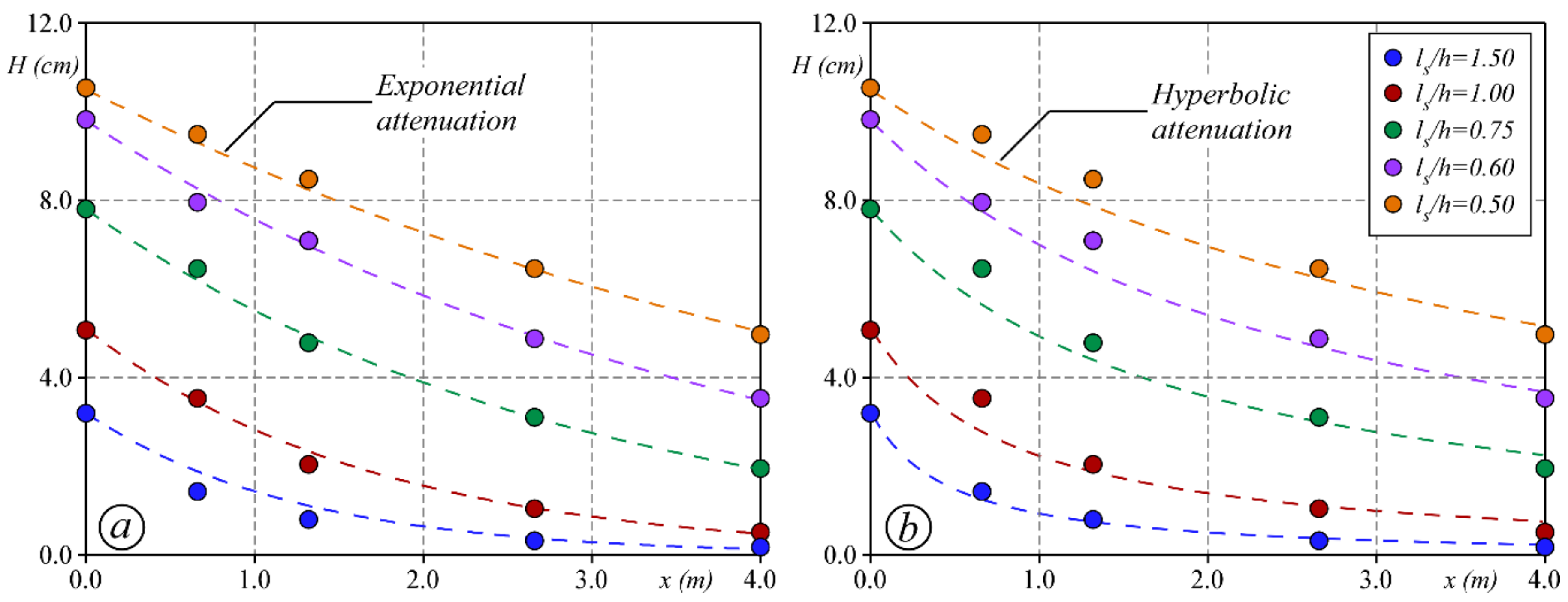
Figure 5 shows an example of wave attenuation when the vegetation density is = 312.5 plant/m2, and the wave period and slope are = 1 s and = 0.08. The attenuation depends on the ratio between vegetation height and water depth, . Since most energy dissipation occurs in the lower part of the water column obstructed by the stems, the capability of damping turns out to be inversely related to the degree of plant submersion. The overall reduction of over the 4 m of Spartina for = 1.5, i.e., for partially emergent condition, is nearly 90% whereas, for = 0.5, i.e., for submerged conditions, the reduction is smaller than 50%.
Figure 5a,b show the experimental data fitted by the exponential law (6) and by the hyperbolic law (4), respectively. The root mean square error due to the hyperbolic law, , is 3.2 mm, while a smaller = 1.7 mm is estimated for the exponential law. The comparison between predicted and measured wave height clearly shows that the exponential law better fits the data. For this reason, the exponential model of wave height attenuation is used in the following discussion.
Also, the stem density, , controls wave attenuation, as indicated by Equation (5). Figure 6 shows the estimated coefficient as a function of . Here, values are the average of all the runs having the same stem density and relative vegetation height, . Interestingly, Figure 6 shows that increases less than linearly with , in spite of what was indicated by Equation (5); this important point is discussed later in the text.
The estimated values for are used, with Equation (5), to estimate the stem drag coefficient, . The latter is shown in Figure 7 as a function of the Reynolds number, , and the Keulegan–Carpenter number, . The stem drag coefficient reduces with as well as with increasing, and can be fitted to the following empirical formulas:
A sensitivity analysis is carried out considering the error due to the measure of the water depth, . Such variation has been estimated at ±0.1 cm and slightly affects the s, whose maximum variation is about ±2% in the tests performed with the minimum water depth (i.e., = 10 cm).
The coefficients of determination for Equations (12) and (13) are = 0.68 and 0.59, respectively; hence the regression of computed provides a better correlation with compared to . However, given the observed scatter of data, the above relationships cannot be used to safely estimate the drag coefficient.
There are two main reasons for this low accuracy. Firstly, the exact definition of the plant impact area per unit of height. This length is the cylinder diameter when the vegetation is simulated by rigid dowels. In the case of Spartina maritima, which is a porous barrier to the flow where stems can overlap each other, forming a net-like structure [41,42], it is only approximatively equal to the stem diameter. Secondly, the parameter considers all the effects that contribute to the overall dissipation process, so a single contribution cannot be distinguished, e.g., the extended wake zone within the stems’ array [50,51,52] and stem flexibility [53].
In order to improve the correlation between the measured and predicted values, Mendez and Losada [26] suggest replacing in Equation (13) with a modified Keulegan–Carpenter number, i.e., , which accounts for the impact of submergence. Anderson and Smith [29] extended the same correction to Equation (12) by replacing with . Close inspection of Figure 7 shows that both these corrections, applied to the present results, are ineffective.
In the present case, some improvement in the estimation of the drag coefficient is achieved by considering the impact of stem density, . In Figure 8, the estimated drag coefficient, , is distinguished for each class of relative stem density, , and, for each density, the experimental data are fitted by Equation (10). The relatively high values of the coefficients of determination ( > 0.90) confirm the overall significant improvement. This result proves that the drag experienced by each single stem reduces with increasing dimensionless density , i.e., with increasing in the present experiments. This causes the coefficient to increase less than linearly, as noted above (see Figure 6).
It is worth noting that the exponent slightly varies with , since it ranges between 0.79 and 0.86 for and between 0.71 and 0.81 for . On the contrary, the coefficient significantly reduces when increases (see the coefficient values reported in Figure 8). By forcing to be constant, the following empirical formulas are found:
Figure 9 shows the comparison between the measured drag coefficient and that computed by Equation (14) (panel a) and Equation (15) (panel b). The data are well arranged along the line of perfect agreement, demonstrating that the proposed formulas can explain the measured values well.
A relevant observation is that the stem drag coefficient in the present experiments is much smaller than the drag coefficient for an isolated cylinder under uniform flow conditions (by approximately one order of magnitude). This is not a new result (see, e.g., [54]), but the reasons for these small s are not yet well understood. The observed large drag reduction can be ascribed to either wave flow unsteadiness and/or the relatively high stem density, as observed above, so that wakes interaction dramatically affects values [54].
To investigate this circumstance in more depth, we use the results of the experiments performed with uniform flow conditions.
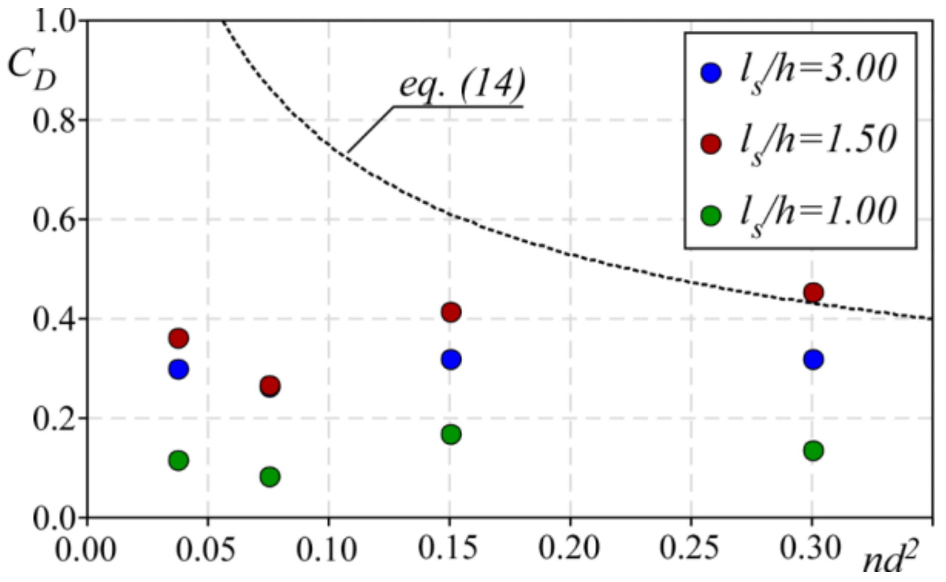
Figure 10 shows the drag coefficient estimated with Equation (11), as it varies with the dimensionless density . The drag coefficient of a smooth isolated cylinder is affected by the wake structure, and depends only on , according to many empirical expressions [55]. For the case of a cylinder array, the downstream elements experience lower impact velocity due to the velocity reduction in the wake of the upstream cylinders; hence, the drag coefficient also depends on cylinder spacing and arrangement. Consequently, the downstream cylinders experience reduced drag. This sheltering effect occurs when the average spacing of the cylinders in the array is relatively small [44]. Consistently, Nepf [25] observed that the bulk drag coefficient remains approximately constant up to values of dimensionless density and then decreases with increasing array density for both random and staggered arrangements; for , the measured drag coefficient scatters in the range . Consequently the present values of are consistent with Nepf’s findings. In our UF experiment, values of are quite invariant with . However, independently of the stem submergence, is at a minimum for ; this may be due to a slight canalization of the flow promoted by the in-line arrangement of the plants (see Figure 4b). Also, the submergence ratio seems to slightly affect the values, perhaps because of the shape of the plants adopted in the tests: their stems gather together in a short basal tuft, thus showing a non-constant impact area along the vertical.
Based on the same artificial vegetation, the comparison between the experimental drag coefficients, one estimated in the presence of waves and the other in uniform flow conditions, could be interesting at this stage. In fact, information derived from both cases could be shared.
The inferred drag coefficients in uniform flow are 4–5 times smaller than the corresponding s estimated in wave conditions at the same Reynolds number ( by Equation (14) for and = 135). The smaller values in uniform flow, as well as the dependency of values on stem density observed in wave conditions, can be ascribed to the hydrodynamic conditions, and, in particular, to the unsteadiness that prevents the wake zone from fully developing in the canopy.
How to relate the drag coefficients to each other in uniform and wave conditions is still an open question that demands specific investigations, the results of which would be useful for building an in-depth understanding of wave attenuation in wetlands, and hence in the controlling of coastal hydrodynamics.
4. Conclusions
The present work investigated the resistance to flow of flexible vegetation in waves and in uniform flow conditions. The experiments highlighted the role of stem density in the wave attenuation process; the drag experienced by each single stem is reduced as the density increases, while the overall resistance, and hence wave attenuation, increases when stem density increases. The stem sheltering effect is possibly why the measured drag coefficient, both under wave and uniform flow conditions, is smaller than the of an isolated cylinder. Interestingly, the drag coefficient measured under wave conditions has the same order of magnitude as that measured in uniform flow, for a comparable Reynolds number and stem density, although the latter turns out to be a little smaller. This circumstance suggests that it could be possible to share knowledge on the drag coefficient from one field to the other; however, this issue needs to be further investigated, possibly by mimicking the vegetation with rigid dowels, in order to reduce the number of degrees of freedom, such as the vegetation flexibility and the non-constant impact area along the vertical.
Both Reynolds () and Keulegan–Carpenter () numbers are found to suitably collapse the measured drag coefficient; the present experimental conditions were such that and were substantially related to each other, thus preventing us from understanding which of the two non-dimensional numbers is best suited to describe the variability of the drag coefficient. This point also deserves further, specific investigation.
Acknowledgments
We wish to acknowledge Ilaria Bernardi and Silvia Capuzzo for their contribution to the experimental investigation.
Author Contributions
P.P. dealt with the theoretical model and wrote the paper; F.D.S. dealt with the model and reviewed the manuscript; A.D. dealt with the model and conceived the experiments; M.M. reviewed and edited the manuscript.
Conflicts of Interest
The authors declare no conflict of interest.
References
- Costanza, R.; d’Arge, R.; De Groot, R.; Farber, S.; Grasso, M.; Hannon, B.; Limburg, K.; Naeem, S.; O’Neill, R.V.; Paruelo, J.; et al. The value of the world’s ecosystem services and natural capital. Nature 1997, 387, 253–260. [Google Scholar] [CrossRef]
- Fonseca, M.S.; Fisher, J.S.; Zieman, J.C.; Thayer, G.W. Influence of the seagrass, Zostera marina L., on current flow. Estuar. Coast. Shelf Sci. 1982, 15, 351–364. [Google Scholar] [CrossRef]
- Fonseca, M.S.; Cahalan, J.A. A preliminary evaluation of wave attenuation by four species of seagrass. Estuar. Coast. Shelf Sci. 1992, 35, 565–576. [Google Scholar] [CrossRef]
- Titus, J.G. Rising seas, coastal erosion, and the takings clause: How to save wetlands and beaches without hurting property owners. MD Law Rev. 1998, 57, 1279–1399. [Google Scholar]
- Carniello, L.; Defina, A.; D’Alpaos, L. Morphological evolution of the Venice lagoon: Evidence from the past and trend for the future. J. Geophys. Res. Earth Surf. 2009, 114. [Google Scholar] [CrossRef]
- Kobayashi, N.; Raichle, A.W.; Asano, T. Wave attenuation by vegetation. J. Waterw. Port Coast. Ocean Eng. 1993, 119, 30–48. [Google Scholar] [CrossRef]
- Mork, M. Wave attenuation due to bottom vegetation. Waves Nonlinear Process. Hydrodyn. 1996, 371–382. [Google Scholar]
- Möller, I.; Spencer, T. Wave dissipation over macro-tidal saltmarshes: Effects of marsh edge typology and vegetation change. J. Coast. Res. 2002, 36, 506–521. [Google Scholar]
- Ghisalberti, M.; Nepf, H.M. Mixing layers and coherent structures in vegetated aquatic flows. J. Geophys. Res. Ocean. 2002, 107. [Google Scholar] [CrossRef]
- Ghisalberti, M.; Nepf, H. The structure of the shear layer in flows over rigid and flexible canopies. Environ. Fluid Mech. 2006, 6, 277–301. [Google Scholar] [CrossRef]
- Palmer, M.R.; Nepf, H.M.; Pettersson, T.J.R. Accumulation and Removal in Aquatic Systems. Limnol. Oceanogr. 2004, 49, 76–85. [Google Scholar] [CrossRef]
- Hendriks, I.E.; Sintes, T.; Bouma, T.J.; Duarte, C.M. Experimental assessment and modeling evaluation of the effects of the seagrass Posidonia oceanica on flow and particle trapping. Mar. Ecol. Prog. Ser. 2008, 356, 163–173. [Google Scholar] [CrossRef]
- Stancanelli, L.M.; Musumeci, R.E.; Cavallaro, L.; Foti, E. A small scale Pressure Retarded Osmosis power plant: Dynamics of the brackish effluent discharge along the coast. Ocean Eng. 2017, 130, 417–428. [Google Scholar] [CrossRef]
- Peruzzo, P.; Defina, A.; Nepf, H. Capillary trapping of buoyant particles within regions of emergent vegetation. Water Resour. Res. 2012, 48. [Google Scholar] [CrossRef]
- Chang, E.R.; Veeneklaas, R.M.; Buitenwerf, R.; Bakker, J.P.; Bouma, T.J. To move or not to move: Determinants of seed retention in a tidal marsh. Funct. Ecol. 2008, 22, 720–727. [Google Scholar] [CrossRef]
- Peruzzo, P.; Defina, A.; Nepf, H.M.; Stocker, R. Capillary interception of floating particles by surface-piercing vegetation. Phys. Rev. Lett. 2013, 111, 164501. [Google Scholar] [CrossRef] [PubMed]
- Peruzzo, P.; Pietro Viero, D.; Defina, A. A semi-empirical model to predict the probability of capture of buoyant particles by a cylindrical collector through capillarity. Adv. Water Resour. 2016, 97, 168–174. [Google Scholar] [CrossRef]
- Gacia, E.; Granata, T.; Duarte, C. An approach to measurement of particle flux and sediment retention within seagrass (Posidonia oceanica) meadows. Aquat. Bot. 1999, 65, 255–268. [Google Scholar] [CrossRef]
- Gacia, E.; Duarte, C.M. Sediment retention by a Mediterranean Posidonia oceanica meadow: The balance between deposition and resuspension. Estuar. Coast. Shelf Sci. 2001, 52, 505–514. [Google Scholar] [CrossRef]
- Fauria, K.E.; Kerwin, R.E.; Nover, D.; Schladow, S.G. Suspended particle capture by synthetic vegetation in a laboratory flume. Water Resour. Res. 2015, 51, 9112–9126. [Google Scholar] [CrossRef]
- De Serio, F.; Meftah, M.B.; Mossa, M.; Termini, D. Experimental investigation on dispersion mechanisms in rigid and flexible vegetated beds. Adv. Water Resour. 2017. [Google Scholar] [CrossRef]
- Mossa, M.; De Serio, F. Rethinking the process of detrainment: Jets in obstructed natural flows. Sci. Rep. 2016, 6, 39103. [Google Scholar] [CrossRef] [PubMed]
- Mossa, M.; Meftah, M.B.; De Serio, F.; Nepf, H.M. How vegetation in flows modifies the turbulent mixing and spreading of jets. Sci. Rep. 2017, 7, 6587. [Google Scholar] [CrossRef] [PubMed]
- Dalrymple, R.A.; Kirby, J.T.; Hwang, P.A. Wave diffraction due to areas of energy dissipation. J. Waterw. Port Coast. Ocean Eng. 1984, 110, 67–79. [Google Scholar] [CrossRef]
- Nepf, H.M. Drag, turbulence, and diffusion in flow through emergent vegetation. Water Resour. Res. 1999, 35, 479–489. [Google Scholar] [CrossRef]
- Mendez, F.J.; Losada, I.J. An empirical model to estimate the propagation of random breaking and nonbreaking waves over vegetation fields. Coast. Eng. 2004, 51, 103–118. [Google Scholar] [CrossRef]
- Augustin, L.N.; Irish, J.L.; Lynett, P. Laboratory and numerical studies of wave damping by emergent and near-emergent wetland vegetation. Coast. Eng. 2009, 56, 332–340. [Google Scholar] [CrossRef]
- Manca, E.; Cáceres, I.; Alsina, J.M.; Stratigaki, V.; Townend, I.; Amos, C.L. Wave energy and wave-induced flow reduction by full-scale model Posidonia oceanica seagrass. Cont. Shelf Res. 2012, 50, 100–116. [Google Scholar] [CrossRef]
- Anderson, M.E.; Smith, J.M. Wave attenuation by flexible, idealized salt marsh vegetation. Coast. Eng. 2014, 83, 82–92. [Google Scholar] [CrossRef]
- Ifuku, M.; Hayashi, H. Development of eelgrass (Zostera marina) bed utilizing sand drift control mats. Coast. Eng. J. 1998, 40, 223–239. [Google Scholar] [CrossRef]
- Moeller, I.; Spencert, T.; French, J.R. Wind wave attenuation over saltmarsh surfaces: Preliminary results from Norfolk, England. J. Coast. Res. 1996, 12, 1009–1016. [Google Scholar]
- Moller, I.; Spencer, T.; French, J.R.; Leggett, D.J.; Dixon, M. Wave transformation over salt marshes: A field and numerical modelling study from north Norfolk, England. Estuar. Coast. Shelf Sci. 1999, 49, 411–426. [Google Scholar] [CrossRef]
- Mazda, Y.; Kobashi, D.; Okada, S. Tidal-scale hydrodynamics within mangrove swamps. Wetl. Ecol. Manag. 2005, 13, 647–655. [Google Scholar] [CrossRef]
- Cassan, L.; Roux, H.; Garambois, P.-A. A Semi-Analytical Model for the Hydraulic Resistance Due to Macro-Roughnesses of Varying Shapes and Densities. Water 2017, 9, 637. [Google Scholar] [CrossRef]
- Dubi, A.; Tørum, A. Wave damping by kelp vegetation. Coast. Eng. 1994, 142–156. [Google Scholar] [CrossRef]
- Knutson, P.L.; Brochu, R.A.; Seelig, W.N.; Inskeep, M. Wave damping in Spartina alterniflora marshes. Wetlands 1982, 2, 87–104. [Google Scholar] [CrossRef]
- Elwany, M.H.S.; O’Reilly, W.C.; Guza, R.T.; Flick, R.E. Effects of Southern California kelp beds on waves. J. Waterw. Port Coast. Ocean Eng. 1995, 121, 143–150. [Google Scholar] [CrossRef]
- Möller, I. Quantifying saltmarsh vegetation and its effect on wave height dissipation: Results from a UK East coast saltmarsh. Estuar. Coast. Shelf Sci. 2006, 69, 337–351. [Google Scholar] [CrossRef]
- Silvestri, S.; Defina, A.; Marani, M. Tidal regime, salinity and salt marsh plant zonation. Estuar. Coast. Shelf Sci. 2005, 62, 119–130. [Google Scholar] [CrossRef]
- Beach, W.P.; Neumeier, U.; Ciavola, P. Flow Resistance and Associated Sedimentary Processes in a Spartina maritima Salt-Marsh. J. Coast. Res. 2004, 20, 435–447. [Google Scholar]
- Defina, A.; Peruzzo, P. Floating particle trapping and diffusion in vegetated open channel flow. Water Resour. Res. 2010, 46. [Google Scholar] [CrossRef]
- Defina, A.; Peruzzo, P. Diffusion of floating particles in flow through emergent vegetation: Further experimental investigation. Water Resour. Res. 2012, 48. [Google Scholar] [CrossRef]
- Yan, N.I. Drag Forces on Vegetation Due to Waves and Currents. Master’s Thesis, Delft University of Technology, Delft, The Netherlands, 2014. [Google Scholar]
- Koch, D.L.; Ladd, A.J.C. Moderate Reynolds number flows through periodic and random arrays of aligned cylinders. J. Fluid Mech. 1997, 349, 31–66. [Google Scholar] [CrossRef]
- Poggi, D.; Katul, G.G.; Albertson, J.D. A note on the contribution of dispersive fluxes to momentum transfer within canopies. Boundary-Layer Meteorol. 2004, 111, 615–621. [Google Scholar] [CrossRef]
- Meftah, M.B.; Mossa, M. Prediction of channel flow characteristics through square arrays of emergent cylinders. Phys. Fluids 2013, 25, 45102. [Google Scholar] [CrossRef]
- Meftah, M.B.; De Serio, F.; Mossa, M. Hydrodynamic behavior in the outer shear layer of partly obstructed open channels. Phys. Fluids 2014, 26, 65102. [Google Scholar] [CrossRef]
- Defina, A.; Bixio, A.C. Mean flow and turbulence in vegetated open channel flow. Water Resour. Res. 2005, 41. [Google Scholar] [CrossRef]
- Poggi, D.; Krug, C.; Katul, G.G. Hydraulic resistance of submerged rigid vegetation derived from first-order closure models. Water Resour. Res. 2009, 45. [Google Scholar] [CrossRef]
- Blevins, R.D. Forces on and Stability of a Cylinder in a Wake. ASME J. Offshore Mech. Arct. Eng. 2005, 127, 39–45. [Google Scholar] [CrossRef]
- Zdravkovich, M.M.; Pridden, D.L. Interference between two circular cylinders; series of unexpected discontinuities. J. Wind Eng. Ind. Aerodyn. 1977, 2, 255–270. [Google Scholar] [CrossRef]
- Tanino, Y.; Nepf, H.M. Laboratory investigation of mean drag in a random array of rigid, emergent cylinders. J. Hydraul. Eng. 2008, 134, 34–41. [Google Scholar] [CrossRef]
- Luhar, M.; Nepf, H.M. Flow-induced reconfiguration of buoyant and flexible aquatic vegetation. Limnol. Oceanogr. 2011, 56, 2003–2017. [Google Scholar] [CrossRef]
- Trimble, S.; Houser, C.; Trimble, S.; Morales, B. Influence of Blade Flexibility on the Drag Coefficient of Aquatic Vegetation. Estuar. Coast. 2015, 38, 569–577. [Google Scholar]
- White, F.M. Viscous Fluid Flow; McGraw-Hill Education: New York, NY, USA, 1991; pp. 335–393. [Google Scholar]
Figure 1.
Scheme of the wave apparatus setup. Distances are in meters.
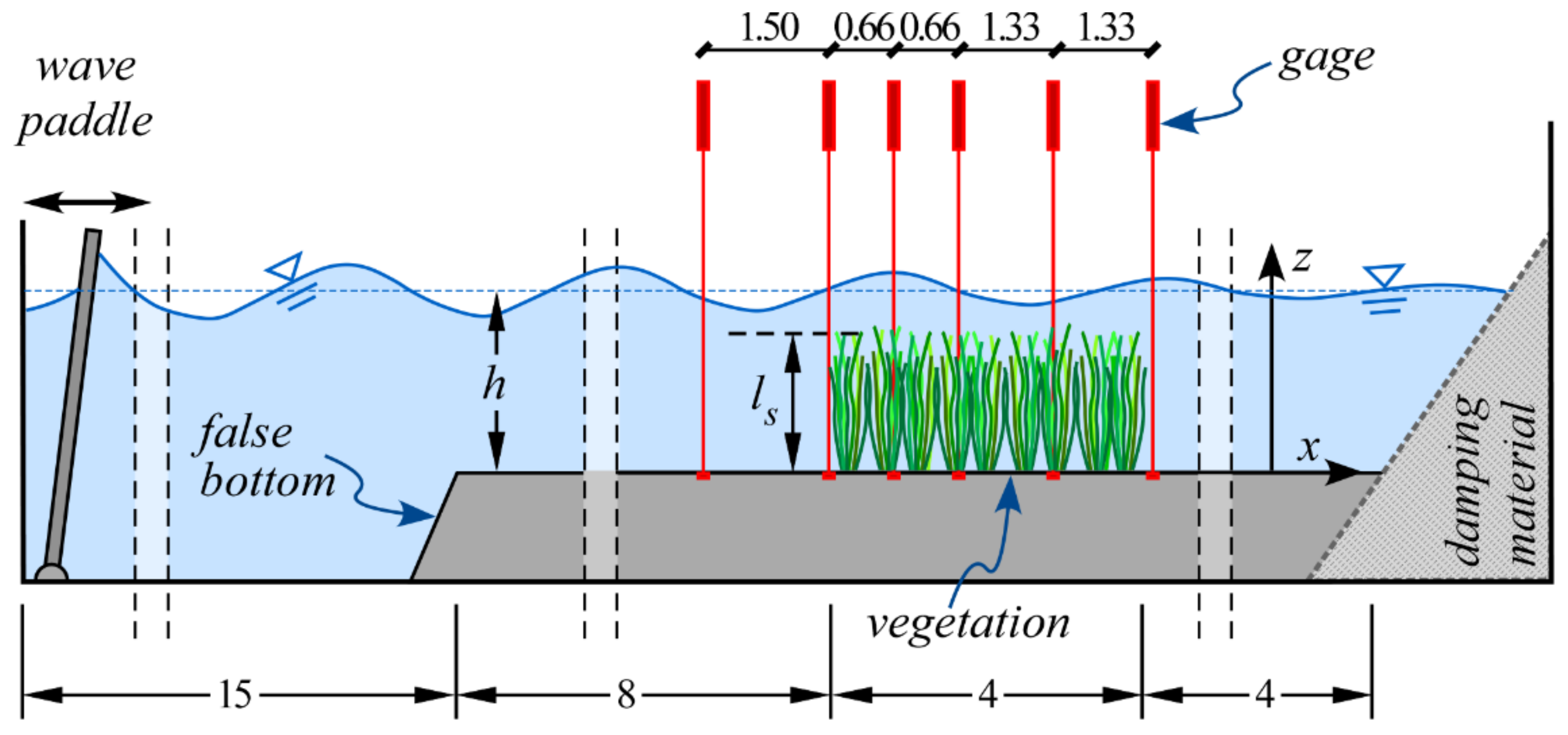
Figure 2.
Vegetation used in the experiments. (a) Plant housing into a drilled PVC panel; (b) comparison between silicone plant (left) and Spartina maritima harvested in the Venice Lagoon (right).
Figure 2.
Vegetation used in the experiments. (a) Plant housing into a drilled PVC panel; (b) comparison between silicone plant (left) and Spartina maritima harvested in the Venice Lagoon (right).
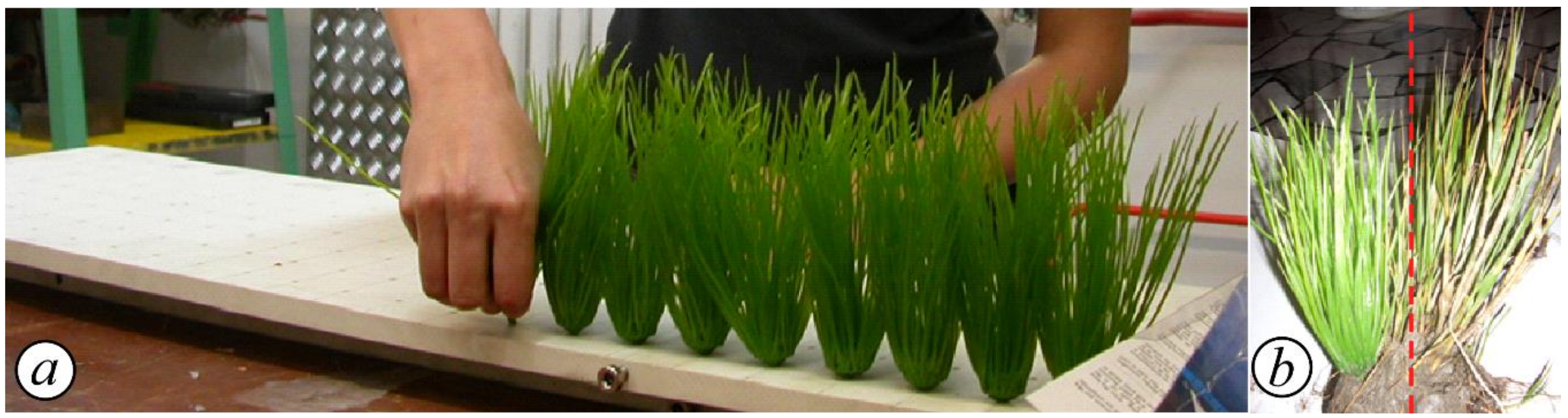
Figure 3.
Plants distribution for the four tested configurations: (a) plants density = 43.75 plant/m2; (b) plants density = 84.5 plant/m2; (c) plants density = 156.25 plant/m2; and (d) plants density = 312.5 plant/m2.
Figure 3.
Plants distribution for the four tested configurations: (a) plants density = 43.75 plant/m2; (b) plants density = 84.5 plant/m2; (c) plants density = 156.25 plant/m2; and (d) plants density = 312.5 plant/m2.
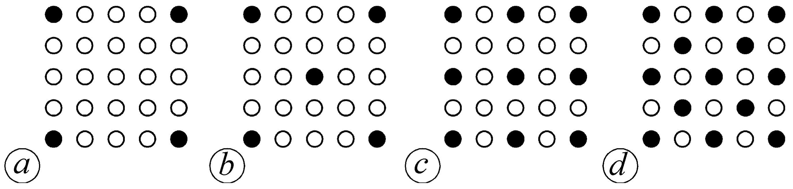
Figure 4.
Plants distribution for the uniform flow tests: (a) plants density = 78.125 plant/m2; (b) plants density = 156.25 plant/m2; (c) plants density = 312.5 plant/m2; and (d) plants density = 625 plant/m2.
Figure 4.
Plants distribution for the uniform flow tests: (a) plants density = 78.125 plant/m2; (b) plants density = 156.25 plant/m2; (c) plants density = 312.5 plant/m2; and (d) plants density = 625 plant/m2.

Figure 5.
Wave height along the vegetated reach when density is = 312.5 plant/m2 and the relative vegetation height is in the range . Wave period and slope are = 1 s and = 0.08. Circles denote the experimental data, dashed line are the modeled wave attenuation either with (a) the exponential model given by Equation (6); or (b) the hyperbolic model given by Equation (4).

Figure 6.
Coefficient of dissipation, , as a function of stem density, . Average are computed for = 1.5 (blue circles), = 1.0 (red circles), = 0.75 (green circles), and = 0.5 (orange circles). Bars show the range of variability of in the present experiments.
Figure 6.
Coefficient of dissipation, , as a function of stem density, . Average are computed for = 1.5 (blue circles), = 1.0 (red circles), = 0.75 (green circles), and = 0.5 (orange circles). Bars show the range of variability of in the present experiments.
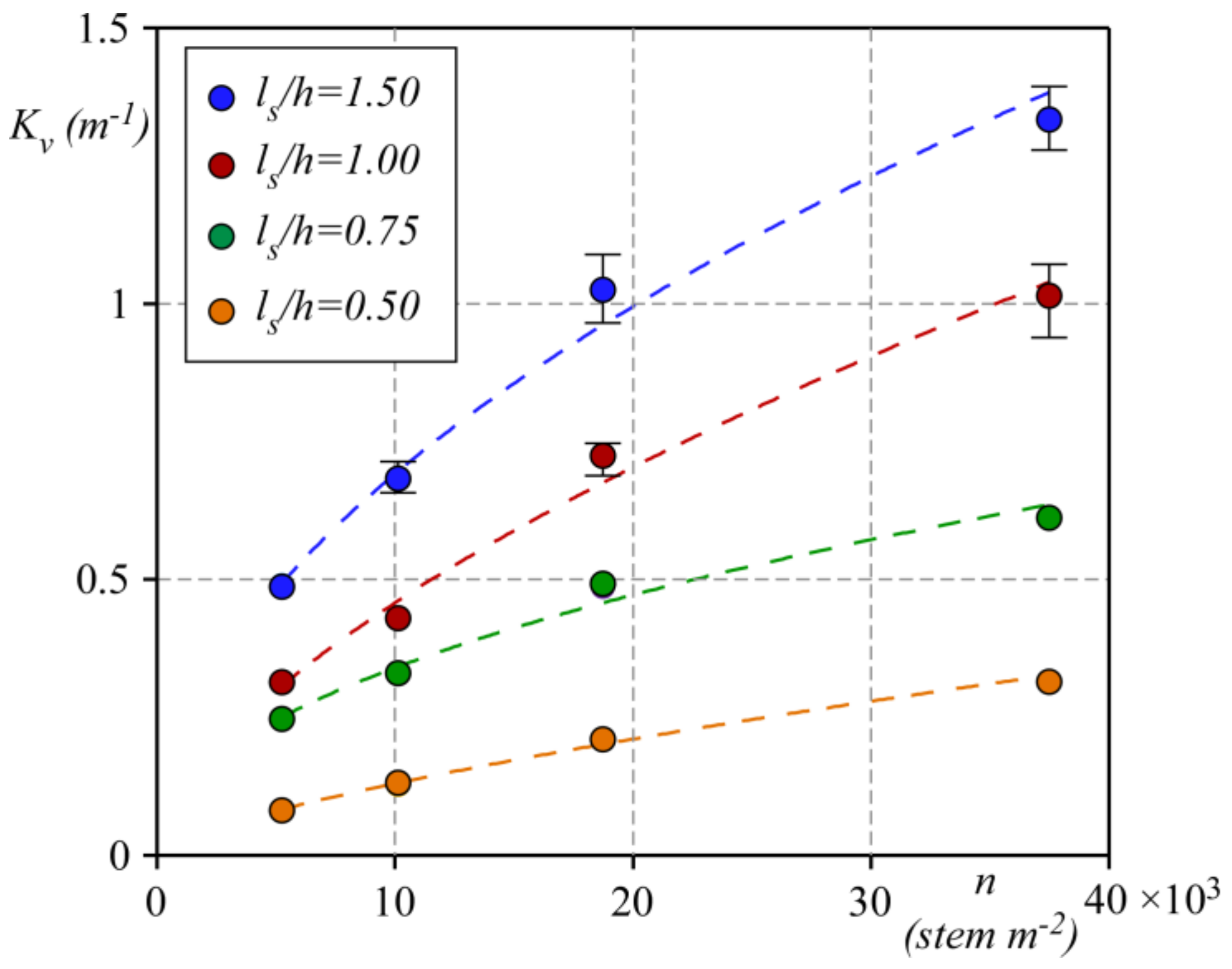
Figure 7.
Drag coefficient, , versus Reynolds number, , (panel (a)) and Keulegan–Carpenter number, , (panel (b)). The solid black line represents the regression of experimental data (circles) according to Equation (10).
Figure 7.
Drag coefficient, , versus Reynolds number, , (panel (a)) and Keulegan–Carpenter number, , (panel (b)). The solid black line represents the regression of experimental data (circles) according to Equation (10).
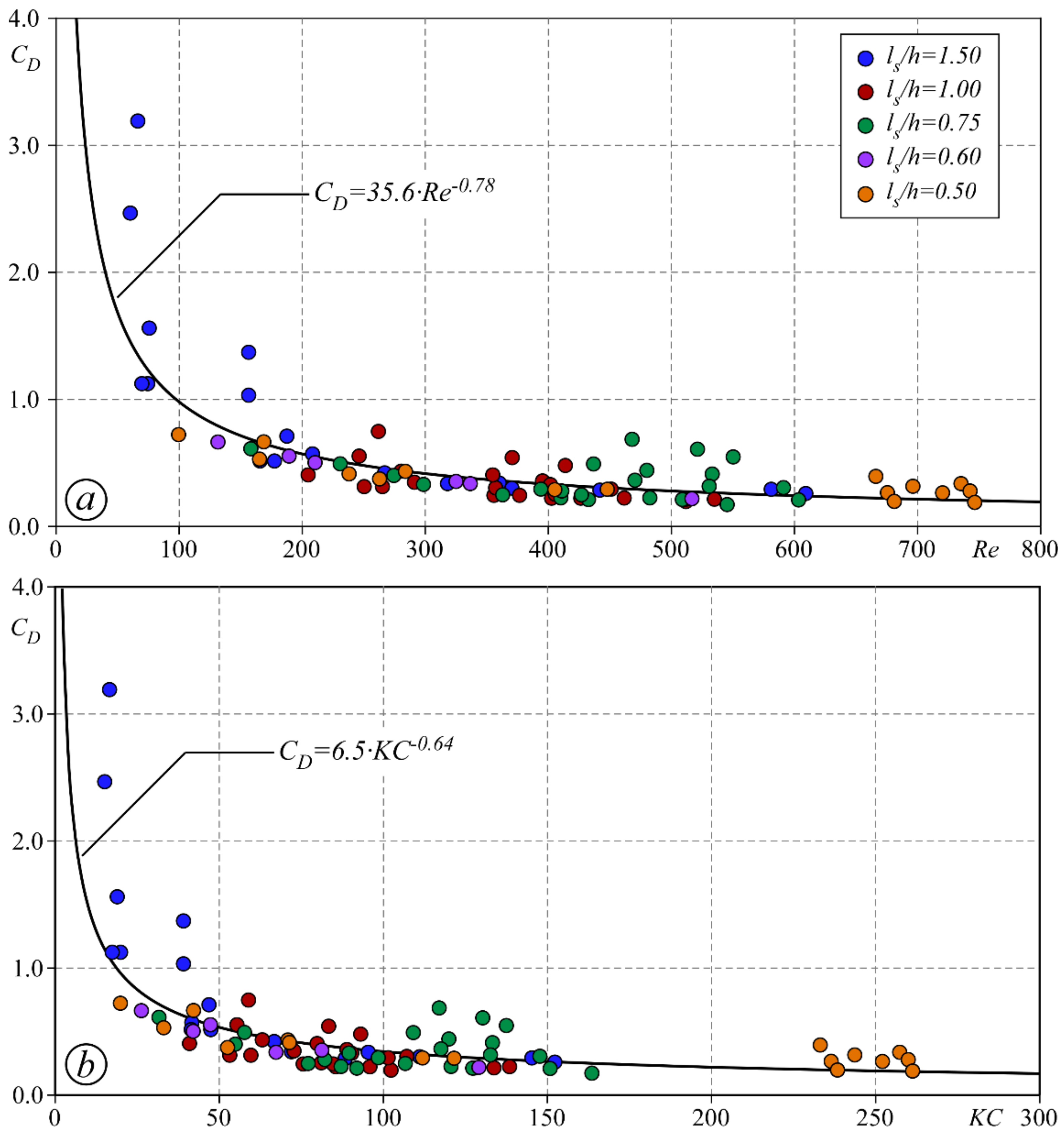
Figure 8.
Predicted drag coefficient, , versus Reynolds number, , (panel (a)) and Keulegan–Carpenter number, , (panel (b)) for the four stem densities. The table in the insets gives the coefficients and to be used in Equation (10).
Figure 8.
Predicted drag coefficient, , versus Reynolds number, , (panel (a)) and Keulegan–Carpenter number, , (panel (b)) for the four stem densities. The table in the insets gives the coefficients and to be used in Equation (10).
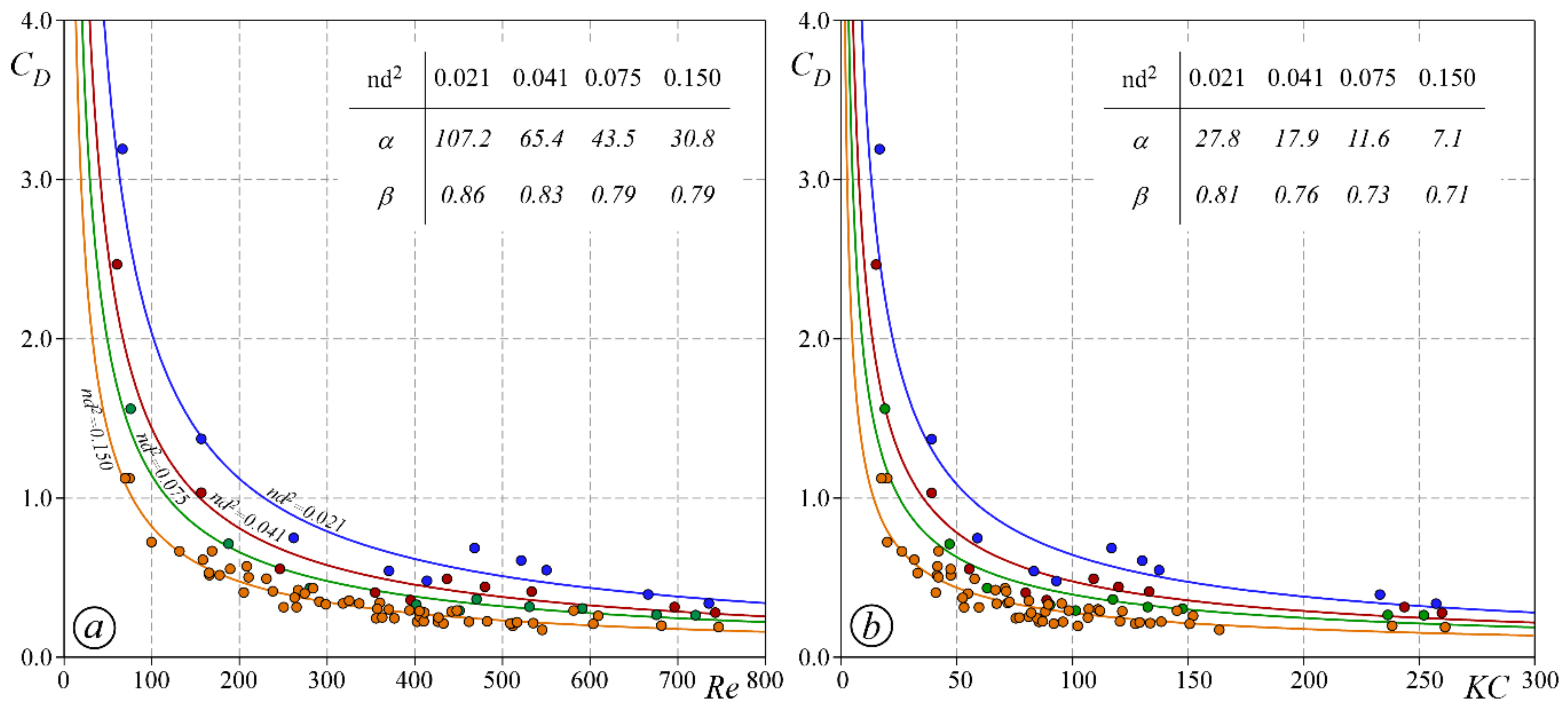
Figure 9.
Predicted versus experimental drag coefficient, ; given by Equation (14) (panel (a)) and by Equation (15) (panel (b)). Solid black line indicates perfect agreement between the data and the empirical formulas.
Figure 9.
Predicted versus experimental drag coefficient, ; given by Equation (14) (panel (a)) and by Equation (15) (panel (b)). Solid black line indicates perfect agreement between the data and the empirical formulas.

Figure 10.
Experimental drag coefficient versus dimensionless density . Dotted black line shows the drag coefficient predicted by Equation (14) for Re = 135 in oscillatory flow.
Figure 10.
Experimental drag coefficient versus dimensionless density . Dotted black line shows the drag coefficient predicted by Equation (14) for Re = 135 in oscillatory flow.


Table 1.
Summary of the tests in wave condition.
| Series 1 | ||||
| np | n | h | T | H0/L |
| (plant/m2) | (stem/m2) | (cm) | (s) | |
| 43.75 | 5250 | 10 ÷ 30 | 0.7 ÷ 1.4 | 0.01 ÷ 0.09 |
| 84.50 | 10,140 | |||
| 156.25 | 18,750 | |||
| 312.50 | 37,500 | |||
| Series 2 | ||||
| 312.50 | 37,500 | 10 ÷ 30 | 0.8; 1.0; 1.2 | 0.03; 0.05; 0.08 |
Table 2.
Summary of the tests in uniform flow condition.
| Uniform Flow Test | |||
|---|---|---|---|
| np | n | h | T |
| (plant/m2) | (stem/m2) | (cm) | (s) |
| 78.125 | 9375 | 5; 10: 15 | ~6.7 |
| 156.25 | 18,750 | ||
| 312.50 | 37,500 | ||
| 625.00 | 75,000 | ||
© 2018 by the authors. Licensee MDPI, Basel, Switzerland. This article is an open access article distributed under the terms and conditions of the Creative Commons Attribution (CC BY) license (http://creativecommons.org/licenses/by/4.0/).
Share and Cite
MDPI and ACS Style
Peruzzo, P.; De Serio, F.; Defina, A.; Mossa, M. Wave Height Attenuation and Flow Resistance Due to Emergent or Near-Emergent Vegetation. Water 2018, 10, 402. https://doi.org/10.3390/w10040402
AMA Style
Peruzzo P, De Serio F, Defina A, Mossa M. Wave Height Attenuation and Flow Resistance Due to Emergent or Near-Emergent Vegetation. Water. 2018; 10(4):402. https://doi.org/10.3390/w10040402
Chicago/Turabian StylePeruzzo, Paolo, Francesca De Serio, Andrea Defina, and Michele Mossa. 2018. "Wave Height Attenuation and Flow Resistance Due to Emergent or Near-Emergent Vegetation" Water 10, no. 4: 402. https://doi.org/10.3390/w10040402
Note that from the first issue of 2016, this journal uses article numbers instead of page numbers. See further details here.