Planning Water Resources in an Agroforest Ecosystem for Improvement of Regional Ecological Function Under Uncertainties

Abstract

In this study, an agroforestry ecosystem project (AEP) is developed for confronting the conflict between agricultural development and forest protection. A fuzzy stochastic programming with Laplace scenario analysis (FSL) is proposed for planning water resources in an AEP issue under uncertainties. FSL can not only deal with spatial and temporal variations of hydrologic elements and meteorological conditions; but also handle uncertainties that are expressed in terms of probability, possibility distributions and fuzzy sets; meanwhile, policy scenario analysis with Laplace’s criterion (PSL) is introduced to handle probability of each scenario occurrence under the supposition of no data available. The developed FSL can be applied to an AEP issue in Xixian county, located in north of China. The result of ecological effects, water allocation patterns, pollution mitigation schemes and system benefits under various scenarios are obtained, which can support policymakers adjusting current strategy to improve regional ecological function with cost-effective and sustainable manners. Meanwhile, it can support generating a robust water plan for regional sustainability in an AEP issue under uncertainties.

1. Introduction

On the context of population growth, agricultural development has great contributed to the satisfaction of increasing food demand. Farming cultivation has been developed at a high speed, with aim to keep the rhythm to population growth and economic development worldwide. On the one hand, more than 70% of global available freshwater has diverted to agriculture in response to cultivated expansion, which can generate the rising pressure for freshwater. On the other hand, the irrational irrigative schedule, fertilization mode, and livestock breeding can accelerate Stalinization, soil erosion, and pollutant discharge. All above can bring about great stresses on water resources and environment, which would challenge policymakers worldwide. Meanwhile, due to irrigative exploration, much land such as forest land has been over-exploited into irrigative land, which would disturb the function of groundcover, leading ecological denegation. In order to confront ecological denegation, agroforestry ecosystem projects (AEP) associated with recovering forest, withdrawing cultivation, and regulating livestock production can be advocated to regain the fragile ecological function. Although AEP is beneficial to regain the ecological services (e.g., nutrient cycling, erosion control, soil fertility, and water conservation) to bring about more intangible ecological benefits to human beings, it can consume numbers of available water in a short-run. It can generate new water competitions between regional agricultural development and forest protection, which would increase the difficulty of AEP promotion [1,2,3]. Therefore, an effective water resources plan in an AEP issue to coordinate agricultural activities and forest protection is required, which can promote the regional ecological function to achieve agriculture-environment sustainability.

However, a practical water resources plan in an AEP issue is often complicated with a number of natural, social, economic, environmental, governmental, and technical uncertainties and their interrelationships, which would generate risks in the decision-making process [4]. Therefore, the consciousness of risk for policymaker is required to confront these uncertainties, which can improve the understanding and grasping capacities of the theory of risk phenomenon in a decision-making process. For example, regional hydrologic cycle and meteorological precipitation can impact ecological function, which can be deemed as spatial and temporal variations (e.g., water flows) existing in system [5,6,7,8,9,10]. These random variations can lead stochastic alteration in benefit fluctuation, which have attracted many researchers to confront such stochastic risk due to random event. For instance, Georgiou and Papamichail (2008) proposed simulated annealing (SA) global optimization with stochastic search algorithm to determine the optimal reservoir water policies, where the rainfall, evapotranspiration, and inflow were considered to be stochastic parameters corresponding to different probability of exceedance [5]. Li et al. (2013) developed a two-stage stochastic programming method for optimizing water allocation in irrigation schedules, which could deal with random stream flows that are represented as chances [6]. Vico and Porporato (2013) designed a probabilistic description model to handle crop development and irrigative water requirements with stochastic rainfall [7]. Zeng et al. (2017) developed a simulation-optimization method to deal with random stream flows and pollution discharges with probabilistic distributions in an irrigation system [9]. All the above stochastic mathematical programming (SMP) is effective to deal with spatial and temporal uncertainties represented as chances or probabilities in water resources planning issues. However, it has difficulties in incorporating other formats of uncertainties presented as possibilistic distributions within an optimization framework.

In a practical water resources plan, uncertain system components such as imprecise water availability and fuzzy ecological effect can be embodied in an AEP system, which would increase the complexity of AEP system [11]. Fuzzy mathematic programming (FMP) can be advocated to handle the decision issue with obscure information, which has advantages to identify vagueness coefficient expressed as possibility distributions in the constraint or objective function [12]. Among them, credibility measure (CM) joined into FMP can deal with fuzziness with possibility and necessity degrees, with aim to improve the abilities of vagueness expression. Nonetheless, in a real case of water resources plan, another impact factor such as risk attitudes of policymakers can influence the decision-making processes, which can not be handled by FMP or credibility measure. In general, the expected targets of a water resources plan can be affected by risk attitudes of decision makers (such as risk seeking/avoiding/neural attitude) easily, which would be caused by the private experiences and personality traits of decision makers. Therefore, a scenario analysis (SA) can be introduced to reflect complex systems under a set of ‘possibility space’ future, which would explore approaching dubious information regarding the interaction between many factors (including risk attitudes) and decision outcomes [13]. In such a “possibility space”, the probability of each scenario that is associated with uncertainties influenced by risk attitudes is random, whereas the data of influence factors is limited [14]. Under this situation, Laplace’s criterion can deal with probability of each scenario occurrence under the supposition of no data available; the probabilities of each scenario appear reasonable to suppose that these are equal [15]. As a matter of fact, numbers of uncertainties and their interactions can aggrandize the complexities of water resources plan in an AEP issue, which would require more comprehensive, complex and ambitious plans. Previously, few study reports were concentrated on coupling mixed methods (e.g., SP, FMP, CM and Laplace criterion) into a framework to deal with multiple uncertainties for water resources planning in an AEP issue.

Therefore, the objective of this study is to propose a fuzzy stochastic programming with Laplace criterion (FSL) for planning water resources in an AEP issue to regain the regional ecological function under uncertainties. FSL can handle random uncertainty regarded as probability distribution; meanwhile, it can deal with fuzziness with credibility measure. It can also reflect random scenario that is associated with risk attitude of decision maker with limited data. The proposed method for water resources planning is applied to a real case of AEP issues in Xixian county, China. Rational water allocation plan for AEP (concluding withdrawing reclamation, recovering forest and regulating livestock production) is advocated to relive regional eco-crisis. A number of scenarios associated with ecological effect levels can be analyzed, which can help the policymakers gaining insight into the tradeoff between the benefits of improvement of ecological function and development of economic objective in the study region. The obtained results can facilitate decision makers adjusting current strategyfor economic development and ecological protection with a robust manner.

2. Methodology

In a water resources plan problem, a policymaker is responsible for allocating water to multiple water users to maximize system benefits under limited water availabilities. Based on practical water consumption situations, the expected target (i.e., promised water) has been pre-regulated to each user at the beginning of planning period. If the water is delivered, then it can bring about economic benefit; otherwise, the user should obtain water from more expensive source or afford economic loss [16]. In general, the available water is a random variable, which would rectify the expected target. Thus, a two-stage stochastic programming (TSP) can build a linkage between expected target and random water availability as follows [12]:

$$\mathrm{Max}f={\displaystyle \sum _{m=1}^{M_1}{\delta }_m{w}_m}-{\displaystyle \sum _{m=1}^{M_2}{\displaystyle \sum _{h=1}^H{p}_h}}{\tau }_m{v}_{mh}$$

(1)

subject to

$${\displaystyle \sum _{m=1}^M{g}_{mn}{w}_m}\le c_n,n=1,2,\dots ,N_1$$

(2)

$${\displaystyle \sum _{m=1}^{M_1}{h}_{mt}{w}_m}+{\displaystyle \sum _{m=1}^{M_2}{h}_{mt}^{\prime }{w}_m}\ge q_h,t=1,2,\dots ,N_2;h=1,2,\dots ,H$$

(3)

$$w_m\ge 0,m=1,2,\dots ,M_1$$

(4)

$${\mathrm{y}}_{mh}\ge 0,m=1,2,\dots ,M_2;h=1,2,\dots ,H$$

(5)

where $w_m$ is vector of first-stage decision variable, which has to be decided before the actual realization of the random variable. When the random event occurs, the second-stage decision variable $v_{mh}$ can rectified the expected target (i.e., first-stage decision variable), where the probability of random event is $p_h$ [17]. $q_h$, ${\delta }_m$, ${\tau }_m$, $g_{mn}$ and $c_n$ are coefficients of constraint. However, in a practical water allocation issue, some parameters are vagueness due to data deficits (such as limited economic data or meteorological data), which can be handled by fuzzy mathematic programming (FMP). Particulary, in the issue that is required high quality of fuzzy expression, fuzzy credibility constrained programming (FCP) can be addressed through fuzzy sets in constraint to express relationship between satisfaction degree and system-failure risk. Let $c_n$ to be a fuzzy parameter in Equation (2), which can be expressed as follows [12]:

$$Cr\{{\displaystyle \sum _{m=1}^M{g}_{mn}{w}_m}\le {\tilde{c}}_n\}\ge \alpha ,n=1,2,\dots ,N_1$$

(6)

Based on the concept of credibility, the relationship between credibility, necessity, and possibility measure can be expressed as follows:

$$Cr\left\{\varsigma \le s\right\}=\frac{1}{2}(Pos\left\{\varsigma \le s\right\}+Nec\left\{\varsigma \le s\right\})$$

(7)

$$Pos\left\{\varsigma \le s\right\}=\underset{u\le s}{\sup }\mu (u)$$

(8)

$$Nec\left\{\varsigma \le s\right\}=1-\underset{u>s}{\sup }\mu (u)$$

(9)

where $\varsigma$ is a fuzzy variable with membership function μ, and let μ and r be real numbers. The possibility of a fuzzy event, which is characterized by $\varsigma \le s$ [18]. Let $\tilde{\varsigma }=(a,b,c)$ be a triangular fuzzy number. According to Equations (7)–(9), the expected value of $\tilde{\varsigma }$ is $(a,b,c)/3$ and the corresponding credibility measure can be expressed as follows:

$$\begin{array}{l}Cr\left\{\tilde{\varsigma }\le r\right\}=\{\begin{array}{cc}0& \mathrm{if}r\le a,\\ \frac{r-a}{2(b-a)}& \mathrm{if}a\le r\le b,\\ \\ \frac{r+c-2b}{2(c-b)}& \mathrm{if}b\le r\le c,\\ 1& \mathrm{if}r\ge c,\end{array}\\ Cr\left\{\tilde{\varsigma }\ge r\right\}=\{\begin{array}{cc}0& \mathrm{if}r\le a,\\ \frac{2b-a-r}{2(b-a)}& \mathrm{if}a\le r\le b,\\ \\ \frac{c-r}{2(c-b)}& \mathrm{if}b\le r\le c,\\ 1& \mathrm{if}r\ge c,\end{array}\end{array}$$

(10)

where $r$ deemed as credibility measure (or level) can reflect relationship between satisfaction degree and system-failure risk, which is more suitable to represent the chance of a fuzzy event than possibility does due to its property of self-dual [12]. For example, an event with maximum possibility 1 might not happen while an event with maximum credibility 1 will surely occur. Furthermore, a fuzzy event with maximum possibility 1 sometimes carries no information, while a fuzzy event with maximum credibility 1 means that the event will happen at the greatest chance [18]. In general, the degree of satisfaction of credibility measure is the level of satisfaction with respect to vagueness in the fuzzy parameter, and it is measured between 0 and 1. Systemic risk is the risk of collapse of an entire system (i.e., system-violated risk), which refers to the probability of a given activity or system to fail to achieve its intended goal and that this failure is detrimental. For instance, if the calculation of fuzzy parameters is over-constrained (no solution can be found), it can bring about system-violated risk. It means that higher degree of satisfaction implied higher possibility to achieve higher systemic benefit, while it can generate higher risk level of systemic failure; vice versa. In general, the credibility level should be greater than 0.5 in response to avoiding improper unsatisfactions and violated risks [12,19]. Thus, $Cr\left\{\varsigma \le s\right\}$ can be expressed as $Cr\left\{\varsigma \le s\right\}\ge \alpha \iff r\ge (2-2\alpha ){\varsigma }_2+(2\alpha -1){\varsigma }_1\iff {\varsigma }_2+(1-2\alpha )({\varsigma }_2-{\varsigma }_1)$. Under these situations, Equation (6) can be transformed as follows:

$${\displaystyle \sum _{m=1}^M{g}_{mn}{w}_m}\le c_n^2+(1-2\alpha )(c_n^2-c_n^1),n=1,2,\dots ,N_1$$

(11)

However, in a real world water resources plan, the input of first-stage decision variable would be affected by many factors (e.g., social, economic and environmental affect). Therefore, scenario analysis (SA) can be joined to reflect interaction between risk attitudes and decision outcomes [14]. In general, the risk attitude of policymaker is deemed as an important influence factor in scenario generation, which can be presented randomness. Thus, a stochastic scenario analysis (SSA) can be expressed as follows:

$$\max E(A_{mn})={\displaystyle \sum _{m=1}^M{P}_m}(\underset{d\in D}{\max }{R}_{mn})={\displaystyle \sum _{m=1}^{m_1}{P}_m}\cdot (\underset{d\in D}{\max }P{S}_{m_{1}n})+{\displaystyle \sum _{m=m_1}^{m_2}{P}_m}\cdot (\underset{d\in D}{\max }C{S}_{m_{2}n})$$

(12)

$$\begin{array}{l}{\displaystyle \sum _{m=1}^{m_1}{P}_m}\cdot (\underset{d\in D}{\max }P{S}_{m_{1}n})={(P_1,P_2,\dots ,P_{m_1})}^{\mathrm{T}}\cdot \left(\begin{array}{cccc}P{S}_{11}& P{S}_{12}& \dots & P{S}_{1n}\\ P{S}_{21}& P{S}_{22}& \dots & P{S}_{2n}\\ \dots & \dots & \dots & \dots \\ P{S}_{m_{1}1}& P{S}_{m_{1}2}& \dots & P{S}_{m_{1}n}\end{array}\right)\end{array}$$

(13)

$$\begin{array}{l}{\displaystyle \sum _{m=m_1}^{m_2}{P}_m}\cdot (\underset{d\in D}{\max }C{S}_{m_{2}n})={(P_{(m_1+1)},P_{(m_1+2)},\dots ,P_{m_2})}^{\mathrm{T}}\cdot \left(\begin{array}{cccc}C{S}_{(m_1+1)1}& C{S}_{(m_1+1)2}& \dots & C{S}_{(m_1+1)n}\\ C{S}_{(m_1+2)1}& C{S}_{(m_1+2)2}& \dots & C{S}_{(m_1+2)n}\\ \dots & \dots & \dots & \dots \\ C{S}_{m_{2}1}& C{S}_{m_{2}2}& \dots & C{S}_{m_{2}n}\end{array}\right)\end{array}$$

(14)

where $E(A_{mn})$ is the decision outcome; $A_n$ is payoff matrix row, ($A_n\in A,n=1,2,\dots ,N$); $P_m$ is probability of each scenario occurrence; d is the option, D is the options, $R_{mn}$ is the overall performance. The progressive scenario ($P{S}_{m_{1}n}$) and conservative scenario ($C{S}_{m^{2}n}$) can be incorporated into a SSA to express the progressive/conservative scenario with risk-seeking/risk-avoiding attitude, m₂ and (m₂ − m₁) are the numbers of progressive/conservative scenarios. However, in the random scenario, due to limited data availability on the probabilities of the various outcomes, policymakers have difficulties in handling the probability of each scenario occurrence. Thus, Laplace’s criterion can be introduced to suppose that the probabilities of each scenario appear reasonable to suppose that these are equal, which can support policymaker computing the expected payoff for each alternative and choose alternatives with maximum values [15]. Thus, a fuzzy stochastic programming with Laplace criterion (FSL) can be presented as follows:

$$\begin{array}{ll}\mathrm{Max}f=& \{\frac{1}{m_2}·\left[\left(\begin{array}{cccc}P{S}_{11}& P{S}_{12}& \dots & P{S}_{1n}\\ P{S}_{21}& P{S}_{22}& \dots & P{S}_{2n}\\ \dots & \dots & \dots & \dots \\ P{S}_{m_{1}1}& P{S}_{m_{1}2}& \dots & P{S}_{m_{1}n}\end{array}\right)+\left(\begin{array}{cccc}C{S}_{(m_1+1)1}& C{S}_{m_{1}2}& \dots & C{S}_{(m_1+1)n}\\ C{S}_{(m_1+2)1}& C{S}_{(m_1+2)2}& \dots & C{S}_{(m_1+2)n}\\ \dots & \dots & \dots & \dots \\ C{S}_{m_{2}1}& C{S}_{m_{2}2}& \dots & C{S}_{m_{2}n}\end{array}\right)\right]\}\\ & \cdot {\displaystyle \sum _{m=1}^{M_1}{\delta }_m\cdot w_m}-{\displaystyle \sum _{m=1}^{M_2}{\displaystyle \sum _{h=1}^H{p}_h\cdot }}{\tau }_m\cdot v_{mh}\end{array}$$

(15)

subject to

$${\displaystyle \sum _{m=1}^M{g}_{mn}{w}_m}\le c_n^2+(1-2\alpha )(c_n^2-c_n^1),n=1,2,\dots ,N_1$$

(16)

$${\displaystyle \sum _{m=1}^{M_1}{h}_{mt}{w}_m}+{\displaystyle \sum _{m=1}^{M_2}{h}_{mt}^{\prime }{w}_m}\ge q_h,t=1,2,\dots ,N_2;h=1,2,\dots ,H$$

(17)

$$w_m\ge 0,m=1,2,\dots ,M_1$$

(18)

$${\mathrm{y}}_{mh}\ge 0,m=1,2,\dots ,M_2;h=1,2,\dots ,H$$

(19)

3. Application

The Xixian county locates in the upper Huaihe River Basin (113°15″ E–114°46″ E, 31°31″ N–32°43″ N), which belongs to Henan province, China. It has an area of 10,191 km², which is composed of 65% mountain area and 35% flat depressions. Since it is in the transition zone between the northern subtropical region and the warm temperate zone, the area is suitable for forest growth. Endemic plants such as Taxodium, Ginko and Metasequoia are grow well with the average annual precipitation 645 mm, which can support the development of wood-processing industry. Meanwhile, crops irrigation, such as grain plant, oil plant, and vegetable and fruit plantations have been developed in recent years, which can improve the quality of human living in the study region. However, the precipitation of study region presented as uneven spatial and temporal distribution, where more than 60% of precipitation concentrates on June to September (flood season). On the context of urbanization, forest lands have been exploited as irrigated lands and urban built-up areas; meanwhile, woods have been felled into urban construction. These situations can satisfy the requirement of food demand and accelerate urbanization greatly, but has brought about eco-crisis. This eco-crisis (i.e., an ecological crisis) occurs when change to the environment of a species or population destabilizes its continued survival, which could be caused by: degradation of an abiotic ecological factor, increased pressures from predation and overpopulation. For instance, by 2015, the regional grain output was 45 × 10³ ton per year, while it has occupied 1.91 × 10⁶ ha land and 73.24 × 10⁶ m³ available water [20]. From 2000 to 2015, the increscent of irrigation has increased land area 3.56 × 10³ km²; while, water deficit of irrigating was 38.13 × 10⁶ m³ at highest [20,21,22,23]. Meanwhile, since the regional farmers want to improve the output of irrigation, fertilization can be popularized. However, unregulated fertilization and irrational irrigative scheme can aggravate severe soil loss and pollution emission, leading environmental destruction. Increasing water demand and exhaust emissions have excessed what natural system can afford. Moreover, the defecation from livestock and over-fertilization from irrigation can accelerate salinization, soil erosion, and pollutant discharge, which can disturb the ecological function in the study region. Various environmental and ecological problems caused by irrational agricultural activities have challenged regional policymakers.

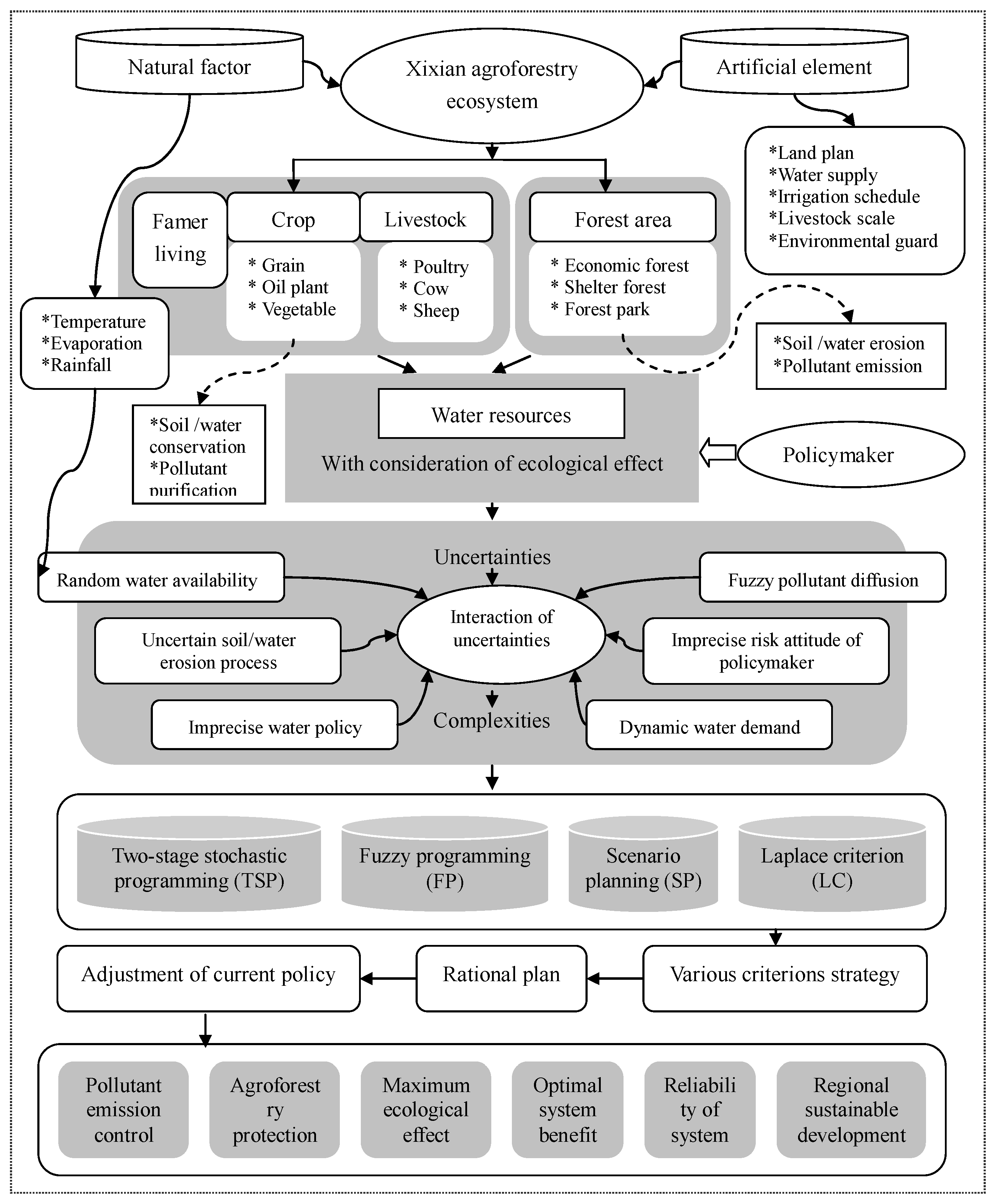
In order to remedy the damage from agricultural activities, an agroforestry ecosystem project (AEP) that is associated with recovering forest, withdrawing cultivation, and regulating livestock production can be advocated. In an AEP issue, farmer living, irrigation, livestock production and forest ecosystem can be incorporated into a framework, where the adverse effects from agricultural activities (e.g., farmer living, crop irrigation, and livestock production) can be transformed by forest system. In an AEP issue, the forest can play an important role in ecological function in the study region, such as flood control, aquifer replenishment, sediment retention, and water filtration. For instance, excessive nitrogen/phosphorus pollutants from excessive fertilization are discharged into water body; then, the forest can purify water and mitigate natural hazards through hydrological cycle, which can provide a diversity of ecosystem as a genetic reserve [24]. Meanwhile, the root system of trees can also give play to water conservation and soil intention, particularly in the flood season. Moreover, economic forest plantation can bring about direct and indirect economic returns to human beings. Based on eco-compensation mechanisms, an AEP issue can be considered an effective manner to regain ecological function and achieve regional sustainability in Xixian county.

Figure 1 presents the relationship among farmer living, crop irrigation, livestock production and forest protection in an AEP issue. In AEP issue, water resources deemed as a key for planning planting scale associated with irrigation withdrawing, livestock regulation, and forest recovery. On the context of limit water availabilities, policymakers should encounter numbers of challenges, as follows: (a) the water consumptions of crop irrigation and livestock production can bring about economic benefits and environmental damages simultaneously. How to develop the ecological effects from forest system to reduce the adverse impacts from agricultural activities would be an important point in an AEP issue; (b) the tradeoff between environmental penalty (the cost for regaining the damages to ecosystem) from agricultural activities and reclamation cost (including lessen of crop planting scale and livestock production size) can facilitate policymakers to generate a compromised water resources plan, which should relieve confrontation between economic development and environmental protection in the study region; and, (c) various strategies for developing orientations can generate different water allocation patterns under varied ecological effects. How to allocate water resources optimally to improve regional ecological functions would be an important part in an AEP issue; (d) since a water resources plan in an AEP issue concludes numbers of uncertainties and their interactions. How to develop a fuzzy two-stage stochastic programming with Laplace scenario analysis (FSL) to deal with the complexities of AEP issues would impact the generation of accurate and irrational water plans. In a practical AEP issue, the imprecise risk attitude of policymaker would impact the decision-making process since the personality traits and previous experiences of policymakers were hard to be calculated accurately. Improper identifications of risk attitudes of policymakers (such as risk-seeking, risk-avoiding, and risk neutral) may influence the generation of rational plans. For instance, a risk-avoiding policymaker can afford a lower risk of system-violation usually. However, if a higher expected target of economic development (agricultural activities) has been pre-regulated for a risk-avoiding policymaker, it can require more demand of water resources, which would result in a higher risk of water deficit exceeding what the risk-avoiding policymaker can not afford; Vice versa. On the context of climate change, the risk of water deficit would be aggravated. Meanwhile, if the expected water demand has been underestimated for a risk-seeking policymaker, it can bring about loss in opportunity cost, which would decrease the total system benefit. Thus, the policymakers should arrange a rational water resources plan compromising speed of economic development and forest protection based on their tolerable risks.

In the study region, policymakers need to make an overall water plan with consideration of ecological effect in an AEP issue to coordinate the relationship between economic development and environmental protection. Meanwhile, the uncertain information should be considered into water plans in order to maximize the system benefit, while minimizing disruption risk that is attributable to uncertainties. Thus, the objective function of water plans in an AEP issue can be expressed as follows:

$$\max {\tilde{f}}_{Laplace}=\{\frac{1}{M}\cdot \left(\begin{array}{cccc}{R}_{11}& R_{12}& \dots & R_{1n}\\ R_{21}& R_{22}& \dots & R_{2n}\\ \dots & \dots & \dots & \dots \\ R_{m1}& R_{m2}& \dots & R_{mn}\end{array}\right)\cdot [(1)+(2)-(3)-(4)-(5)+(6)]$$

(20)

Equation (20) presents the maximum of system benefit under Laplace criterion (${\tilde{f}}_{Laplace}$), which can reflect random scenario associated with risk attitude of policymakers (as shown in Section 2). The total system benefit would equal to benefit from agricultural activity minus loss for water shortage and penalty for environmental pollution; meanwhile, adding to benefit from forest system and benefit from ecological effect. The details of function can be expressed as follows:

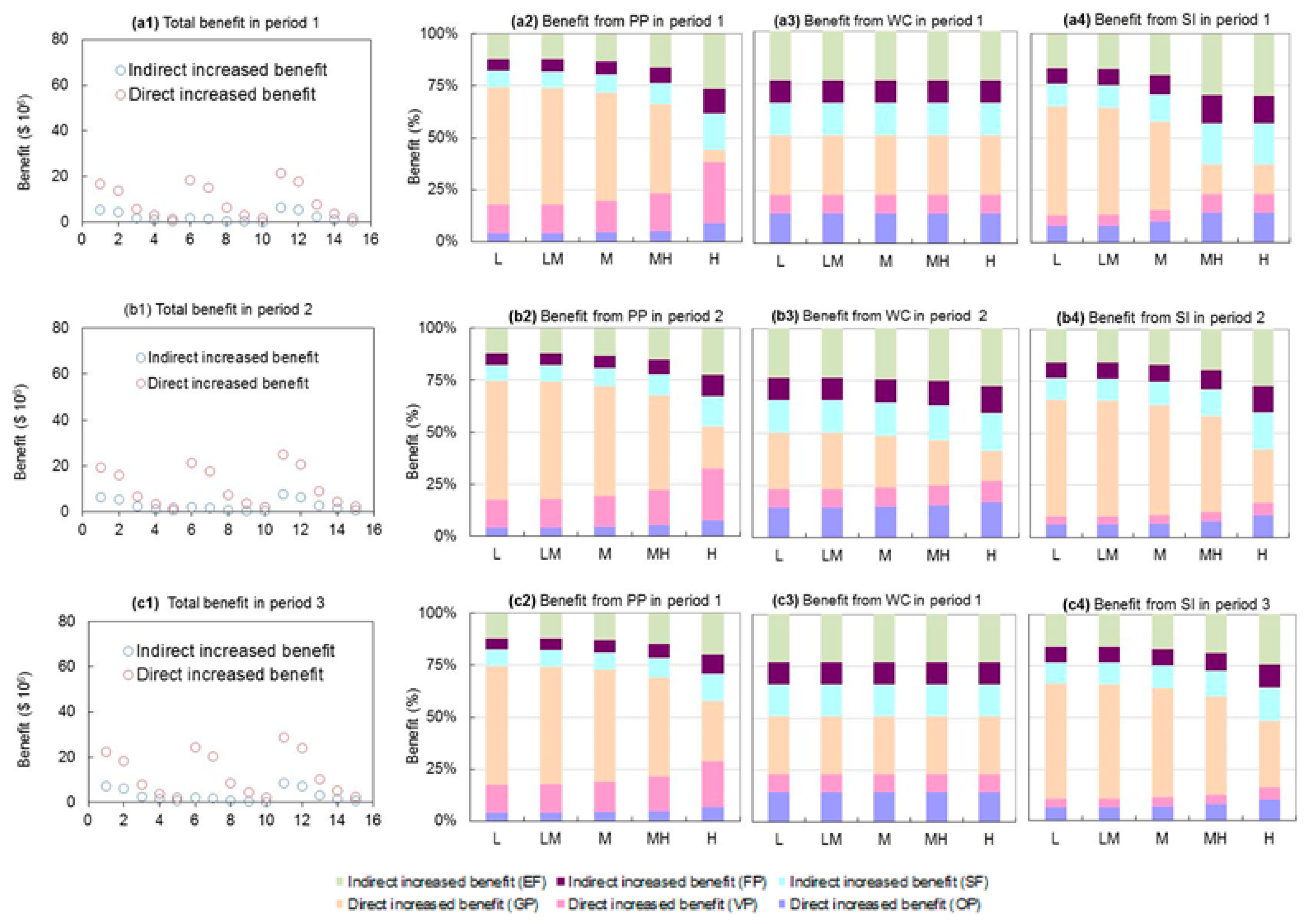
(1) Expected benefit from agricultural activities (including famer living, crop irrigation and livestock production)

$${\displaystyle \sum _{t=1}^3{\displaystyle \sum _{m=1}^1\tilde{b}{m}_{tm}\cdot W{M}_{tm}\cdot \varsigma }}+{\displaystyle \sum _{t=1}^3{\displaystyle \sum _{i=1}^3\tilde{b}{i}_{ti}\cdot W{I}_{ti}\cdot }\tau +}{\displaystyle \sum _{t=1}^3{\displaystyle \sum _{n=1}^3\tilde{b}{a}_{tn}\cdot W{A}_{tn}}}\cdot \xi$$

(21)

In this study, the water consumers in agricultural activities conclude famer living, crop irrigation, and livestock production, which can generate economic benefits. The expected benefit from agricultural activities can be the first-stage variables, which have been regulated before random events occurred. Among them, three main crop types (n = 1 grain (ha), n = 2 oil plants (ha), n = 3 vegetable (ha)) and three livestock varieties (i = 1 cow (head), i = 2 sheep (head) and i = 3 poultry (one)) can be considered. Equation (21) presents that system benefits from agricultural activities would equal to planning developing scales of population, livestock, and irrigation ($W{M}_{tm}$ (people), $W{I}_{ti}$ (head) and $W{A}_{tn}$ (ha)) multiple water use coefficients ($\varsigma$, $\tau$ and $\xi$) multiple net benefit ($b{m}_{tm}$, $b{i}_{ti}$ and $b{a}_{tn}$ ($/ha)). Since economic data estimation is easier to be impacted by anthropogenic and inherent factors, it is expressed as fuzzy set. Three planning periods (t = 1 period 1, t = 2 period 2, t = 3 period 3) can be considered, where three years is one planning period. Under each period, the water demand for agricultural activities can be satisfied, it can achieve goal of economic development.

(2) Expected direct benefit from forest system

$${\displaystyle \sum _{t=1}^3{\displaystyle \sum _{k=1}^3\tilde{b}{e}_{tk}\cdot W{E}_{tk}\cdot \delta }}$$

(22)

Equation (22) presents that expected direct economic benefit can be achieved from forest if water is delivered to forest system. This expected direct benefit is from regional wood-processing industry plan, which is calculated by net benefit of wood ($b{e}_{tk}$ ($/ha)) multiple planting scale ($W{e}_{tk}$ (ha)) multiple water use coefficient ($\delta$).

(3) Loss for water deficit

$${\displaystyle \sum _{h=1}^5{p}_{th}}\cdot [{\displaystyle \sum _{t=1}^3{\displaystyle \sum _{m=1}^1\tilde{l}{m}_{tm}\cdot S{M}_{tmh}\cdot \varsigma }}+{\displaystyle \sum _{t=1}^3{\displaystyle \sum _{i=1}^1\tilde{l}{i}_{ti}\cdot S{I}_{tih}\cdot }\tau +}{\displaystyle \sum _{t=1}^3{\displaystyle \sum _{n=1}^4\tilde{l}{a}_{tn}\cdot S{A}_{tnh}}}\cdot \xi +{\displaystyle \sum _{t=1}^3{\displaystyle \sum _{k=1}^3\tilde{l}{e}_{tk}\cdot S{E}_{tkh}\cdot \delta }}]$$

(23)

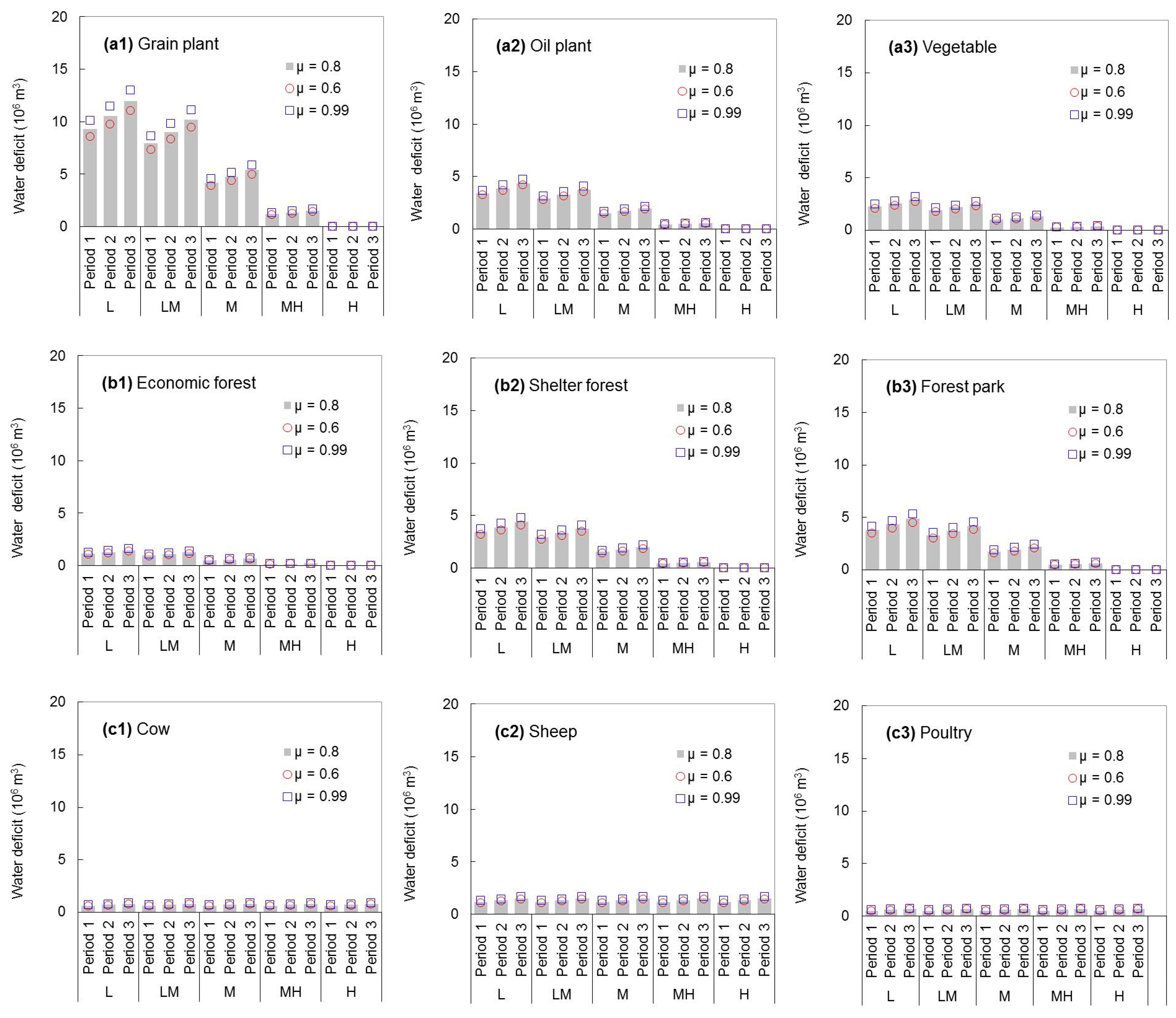
In this study, the available water deemed as random variable can be expressed as varied water levels (i.e., h = 1–5 represent as low, low-medium, medium, medium-high, and high levels). The limited water availability can influence the agricultural development and forest protection, leading water deficit. When the event of water deficit occur, it has taken a recourse action (e.g., loss of water deficit) to the first-stage decision, where $p_{th}$ is the probability for occurrence of scenario p during period t (%). Under various probability levels ($p_{th}$), the losses for water deficit equal to unit losses of water deficit ($l{m}_{tm}$, $l{i}_{ti}$, $l{a}_{tn}$ and $l{e}_{tk}$) multiple ($S{M}_{tmh}$ (people), $S{I}_{tih}$ (head), $S{A}_{tnh}$ (ha) and $S{E}_{tkh}$ (ha)) multiple water use coefficients ($\varsigma$, $\tau$, $\xi$ and $\delta$) in period t ($/p).

(4) Penalty for environmental pollution

$$\begin{array}{l}{\displaystyle \sum _{h=1}^5{p}_{th}}\cdot \{[{\displaystyle \sum _{t=1}^3{\displaystyle \sum _{m=1}^1\tilde{p}n{m}_{tm}^N\cdot (W{M}_{tm}-S{M}_{tmh})\cdot \varsigma }}\cdot PM{N}_{tm}^N+{\displaystyle \sum _{t=1}^3{\displaystyle \sum _{i=1}^1\tilde{p}n{i}_{ti}^N\cdot (W{I}_{ti}-S{I}_{tih})\cdot }\tau }\cdot PI{N}_{ti}^N\\ +{\displaystyle \sum _{t=1}^3{\displaystyle \sum _{n=1}^4\tilde{p}n{a}_{tn}\cdot (W{A}_{tn}-S{A}_{tnh}}})\cdot \xi \cdot PA{N}_{tn}^N]+[{\displaystyle \sum _{t=1}^3{\displaystyle \sum _{m=1}^1\tilde{p}p{m}_{tm}^P\cdot (W{M}_{tm}-S{M}_{tmh})\cdot \varsigma }}\cdot PM{P}_{tm}^P\\ +{\displaystyle \sum _{t=1}^3{\displaystyle \sum _{i=1}^1\tilde{p}p{i}_{ti}^P\cdot (W{I}_{ti}-S{I}_{tih})\cdot }\tau }\cdot PI{P}_{ti}^P+{\displaystyle \sum _{t=1}^3{\displaystyle \sum _{n=1}^4\tilde{p}p{a}_{tn}^P\cdot (W{A}_{tn}-S{A}_{tnh}}})\cdot \xi \cdot PA{P}_{tn}^P]+\\ [{\displaystyle \sum _{t=1}^3{\displaystyle \sum _{m=1}^1\tilde{p}b{m}_{tm}^{BOD}\cdot (W{M}_{tm}-S{M}_{tmh})\cdot \varsigma }}\cdot PM{B}_{tm}^{BOD}+{\displaystyle \sum _{t=1}^3{\displaystyle \sum _{i=1}^1\tilde{p}b{i}_{ti}^{BOD}\cdot (W{I}_{ti}-S{I}_{tih})\cdot }\tau }\cdot PI{B}_{ti}^{BOD}\\ +{\displaystyle \sum _{t=1}^3{\displaystyle \sum _{n=1}^4\tilde{p}b{a}_{tn}^{BOD}\cdot (W{A}_{tn}-S{A}_{tnh}}})\cdot \xi \cdot PA{B}_{tn}^{BOD}]\}\end{array}$$

(24)

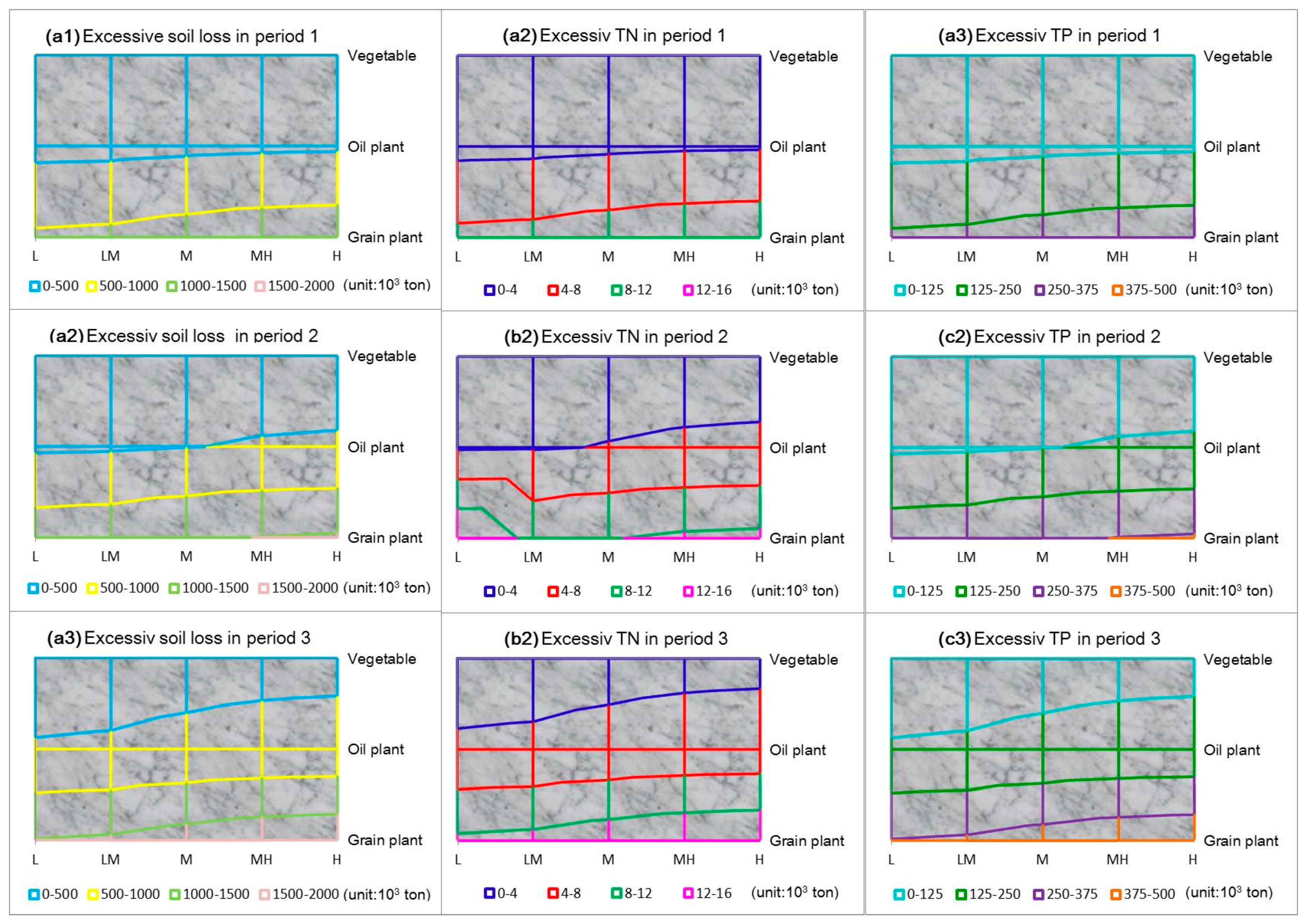
Equation (24) shows the penalty for environmental pollution, which can be calculated as the cost for retreating these pollutions (total nitrogen, total phosphorus, and biochemical oxygen demand, denoted as TN, TP, and BOD) discharge through artificial sewage disposal plant (US $). Where $pn{m}_{tm}^N$/$pp{m}_{tm}^P$/$pb{m}_{tm}^B$, $pn{a}_{tn}^N$/$pp{a}_{tn}^P$/$pb{a}_{tn}^B$, and $pn{i}_{tn}^N$/$pp{i}_{tn}^P$/$pb{i}_{tn}^B$ are unit pollution treatment costs for farmer living, irrigation, and livestock production if TN/TP/BOD discharge being retreated artificial sewage disposal plants in period t ($/ton). $PM{N}_{tm}^N$/$PM{P}_{tm}^P$/$PM{B}_{tm}^B$, $PA{N}_{tn}^N$/$PA{P}_{tn}^P$/$PA{B}_{tn}^B$, and $PI{N}_{tn}^N$/$PI{P}_{tn}^P$/$PI{B}_{tn}^B$, represented as TN/TP/BOD discharge rates of per person/ha/head from farmer living, irrigation and livestock sectors in period t (ton/p or ha or head).

(5) Loss for water and soil erosion

$${\displaystyle \sum _{h=1}^5{p}_{th}}\cdot \{[{\displaystyle \sum _{t=1}^3{\displaystyle \sum _{n=1}^4\tilde{w}{a}_{tn}\cdot (W{A}_{tn}-S{A}_{tnh}}})\cdot E{W}_{tn}]+[{\displaystyle \sum _{t=1}^3{\displaystyle \sum _{n=1}^4\tilde{s}{a}_{tn}\cdot (W{A}_{tn}-S{A}_{tnh}}})\cdot S{W}_{tn}]\}$$

(25)

Equation (25) presents loss for water and soil erosion in response to damage of crop irrigation. Where $E{W}_{tn}$ and $S{W}_{tn}$ are the coefficients of water loss and soil erosion in the study region; $w{a}_{tn}$ and $s{a}_{tn}$ are the unit losses of a water loss and soil erosion per unit water consumption.

(6) Benefit from ecological effect (indirect benefits from forest system)

$$\begin{array}{l}{\displaystyle \sum _{t=1}^3{\displaystyle \sum _{n=1}^{4}BA{A}_{tn}\cdot [(D{A}_{tn}^N}}+D{A}_{tn}^P+D{A}_{tn}^B)+SI{A}_{tn}+WI{A}_{tn}]\cdot WE{A}_{tn}+{\displaystyle \sum _{t=1}^3{\displaystyle \sum _{k=1}^{4}BA{E}_{tk}\cdot [(D{E}_{tk}^N}}+\\ D{E}_{tk}^P+D{E}_{tk}^B)+SI{E}_{tk}+WI{E}_{tk}]\cdot WE{E}_{tn}\end{array}$$

(26)

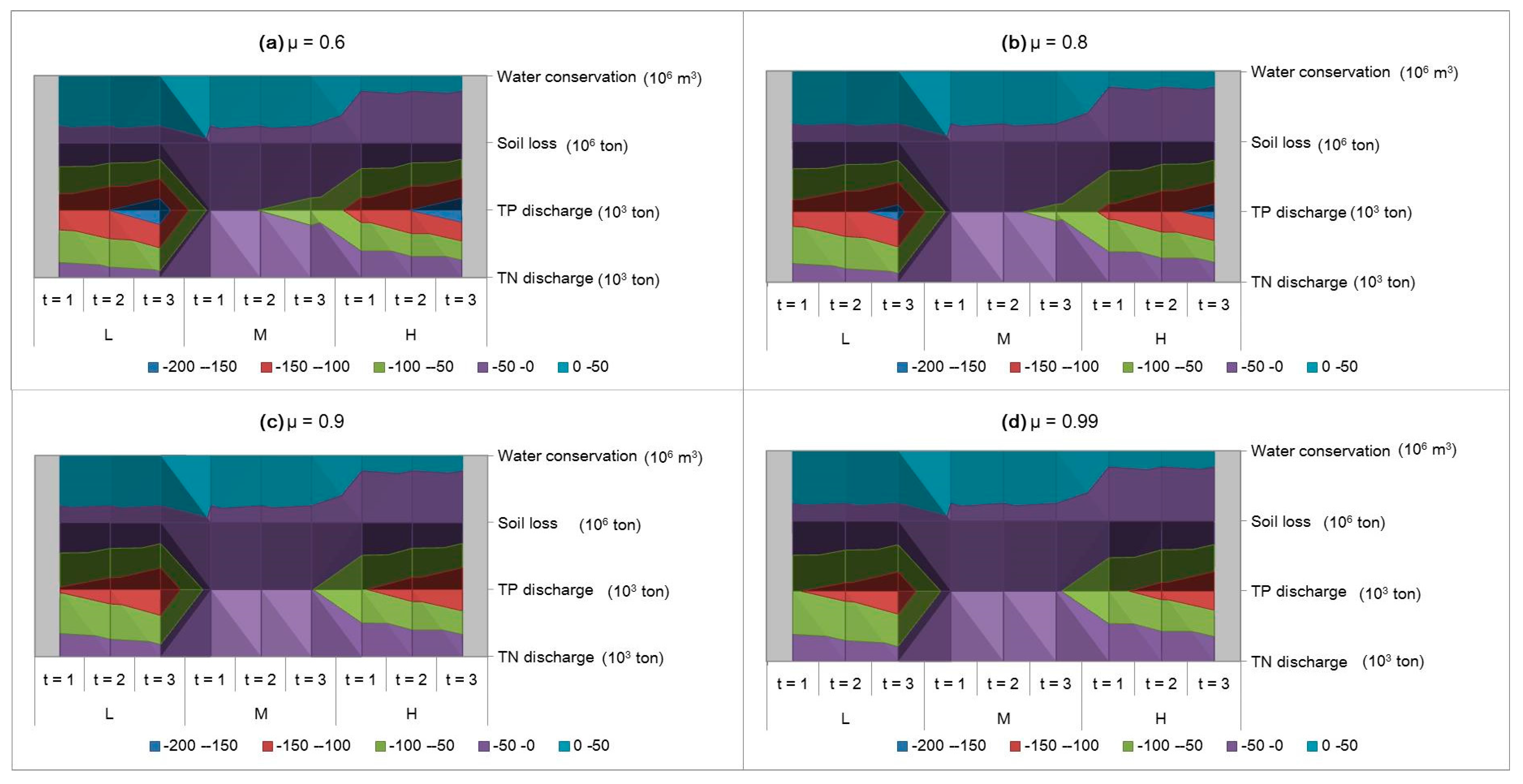
Since forest system can regain the ecological function, such as flood control, aquifer replenishment, sediment retention, and water filtration, which can reduce the damage from agricultural activity. Therefore, model (6f) shows the indirect benefit from forest system due to its ecological effect. Among them, $D{A}_{tn}^N$/$D{A}_{tn}^P$/$D{A}_{tn}^B$ and $D{E}_{tn}^N$/$D{E}_{tn}^P$/$D{E}_{tn}^B$ are the coefficients of purification capacities for TN/TP/BOD discharge in agricultural activities (including famer living, crop irrigation, and livestock production) through ecological mechanism in period t (ton); $SI{A}_{tn},SI{E}_{tk},WI{A}_{tn}$, and $WI{E}_{tk}$ are soil intention and water conservation coefficients from forest system.

Meanwhile, a number of constraints including inequalities associated with water quantity, water nitrogen/phosphorus/BOD discharges, ecological function, and technique constraints can be expressed as follows:

(1) Water quantity

$$\begin{array}{l}Cr\{[{\displaystyle \sum _{t=1}^3{\displaystyle \sum _{m=1}^{1}W{M}_{tm}\cdot \varsigma }}+{\displaystyle \sum _{t=1}^3{\displaystyle \sum _{i=1}^{1}W{I}_{ti}\cdot }\tau +}{\displaystyle \sum _{t=1}^3{\displaystyle \sum _{n=1}^{3}W{A}_{tn}}}\cdot \xi +{\displaystyle \sum _{t=1}^3{\displaystyle \sum _{k=1}^{3}W{E}_{tk}\cdot \delta }}]-{\displaystyle \sum _{p=1}^5{p}_{th}}\cdot [{\displaystyle \sum _{t=1}^3{\displaystyle \sum _{m=1}^{1}S{M}_{tmh}\cdot \varsigma }}\\ +{\displaystyle \sum _{t=1}^3{\displaystyle \sum _{i=1}^{3}S{I}_{tih}\cdot }\tau +}{\displaystyle \sum _{t=1}^3{\displaystyle \sum _{n=1}^{3}S{A}_{tnh}}}\cdot \xi +{\displaystyle \sum _{t=1}^3{\displaystyle \sum _{k=1}^{3}S{E}_{tk}\cdot \delta }}]\le [({\displaystyle \sum _{t=1}^3{\displaystyle \sum _{p=1}^5{\widetilde{QF}}_{th}}}+{\displaystyle \sum _{t=1}^3{\displaystyle \sum _{p=1}^5{\widetilde{QG}}_{th})}}-E_{th}-\\ {\displaystyle \sum _{t=1}^3{\displaystyle \sum _{k=1}^3(1-\alpha )\cdot WE{E}_{tk}}}\cdot RE{C}_{tk}\cdot R{O}_{tk}-H_{th}]\}\ge \mu \end{array}$$

(27)

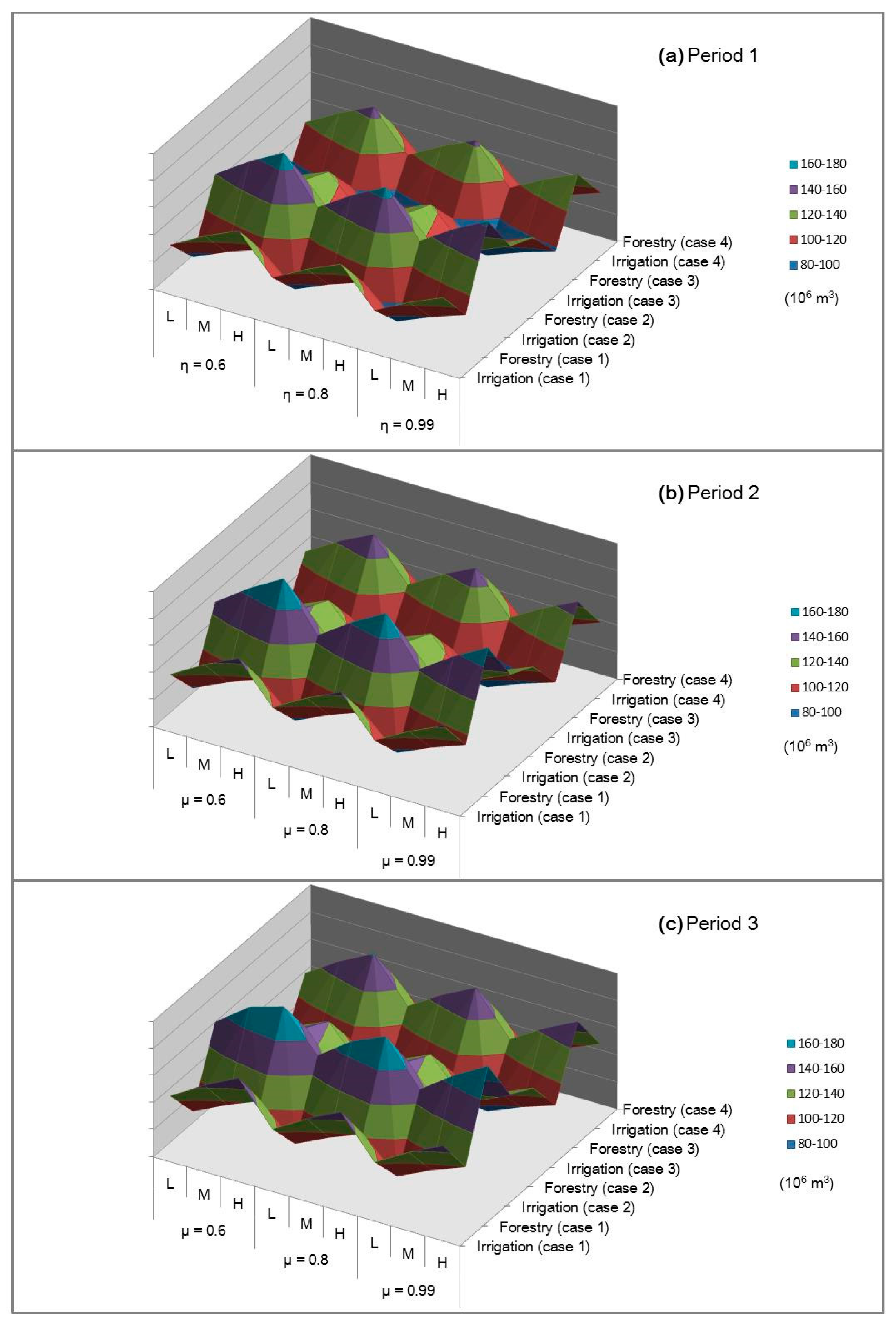
The left-hand side of Equation (27) shows that the expected water demand target can be rectified by the occurrence of water deficit when water is limited. The right-hand side of Equation (27) presents actual water resource loads in the study region, which are composed of total availabilities from surface and underground (i.e., ${\displaystyle \sum _{t=1}^3{\displaystyle \sum _{p=1}^5{\widetilde{QF}}_{th}}}+{\displaystyle \sum _{t=1}^3{\displaystyle \sum _{p=1}^5{\widetilde{QG}}_{th}}}$); meanwhile, evaporation/infiltration (i.e., $E_{th}$), water requirement of watercourse (i.e., $H_{th}$), and minimum ecological water (i.e., ${\displaystyle \sum _{t=1}^3{\displaystyle \sum _{k=1}^3(1-\alpha )\cdot WE{E}_{tk}}}\cdot RE{C}_{tk}\cdot R{O}_{tk}$) should be removed (m³). Since future water availability can be influenced by spatio-temporal factors, a fuzzy credibility programming can be introduced to express uncertain water availability, which can be explained in “Methodology” section.

(2) Water conservation and soil intention capacity under ecological effect

$${\displaystyle \sum _{t=1}^3{\displaystyle \sum _{n=1}^4(W{A}_{tn}-S{A}_{tnh}}})\cdot E{W}_{tn}\le LW{T}_t$$

(28)

$${\displaystyle \sum _{t=1}^3{\displaystyle \sum _{n=1}^4(W{A}_{tn}-S{A}_{tnh}}})\cdot S{W}_{tn}\le LS{T}_t$$

(29)

Equations (28) and (29) present that actual water conservation and soil intension under ecological effects should be less than the maximum capacities of forest ecosystem (i.e., $LW{T}_t$ and $LS{T}_t$). Among them, the coefficients of water conservation and soil intension (i.e., $E{W}_{tn}$ and $S{W}_{tn}$) can influence the capacity of water conservation and soil intension, which have been calculated by previous research works.

(3) Pollution purification capacity under ecological effect

$$\begin{array}{l}{\displaystyle \sum _{h=1}^5{p}_{th}}\cdot [{\displaystyle \sum _{t=1}^3{\displaystyle \sum _{m=1}^1(D{M}_{tm}^N+}}D{M}_{tm}^P+D{M}_{tm}^B)+{\displaystyle \sum _{t=1}^3{\displaystyle \sum _{n=1}^3(D{A}_{tn}^N}}+D{A}_{tn}^P+D{A}_{tn}^B)\\ +{\displaystyle \sum _{t=1}^3{\displaystyle \sum _{i=1}^3(D{I}_{ti}^N+D{I}_{ti}^P+}}D{I}_{ti}^B)]\le (N{P}_t+N{N}_t+{\alpha }_t^{BOD}+{\beta }_t^{BOD})\cdot {\displaystyle \sum _{p=1}^5{p}_{th}}\cdot [{\displaystyle \sum _{t=1}^3{\displaystyle \sum _{k=1}^3(W{E}_{tk}}}-S{E}_{tkh})]\end{array}$$

(30)

(4) Total nitrogen allowance

$$\begin{array}{l}Cr\{{\displaystyle \sum _{h=1}^5{p}_{th}}\cdot \{[{\displaystyle \sum _{t=1}^3{\displaystyle \sum _{m=1}^1(W{M}_{tm}-S{M}_{tmh})\cdot \varsigma }}\cdot PM{N}_{tm}^N+{\displaystyle \sum _{t=1}^3{\displaystyle \sum _{i=1}^3(W{I}_{ti}-S{I}_{tih})\cdot }\tau }\cdot PI{N}_{ti}^N+\\ {\displaystyle \sum _{t=1}^3{\displaystyle \sum _{n=1}^3(W{A}_{tn}-S{A}_{tnh}}})\cdot \xi \cdot PA{N}_{tn}^N]\cdot (1-N{N}_t)\le {\widetilde{tnp}}_{tp}\}\ge \mu \end{array}$$

(31)

(5) Total phosphorus allowance

$$\begin{array}{l}Cr\{[{\displaystyle \sum _{t=1}^3{\displaystyle \sum _{m=1}^1(W{M}_{tm}-S{M}_{tmh})\cdot \varsigma }}\cdot PM{P}_{tm}^P+{\displaystyle \sum _{t=1}^3{\displaystyle \sum _{i=1}^3(W{I}_{ti}-S{I}_{tih})\cdot }\tau }\cdot PI{P}_{ti}^P+\\ {\displaystyle \sum _{t=1}^3{\displaystyle \sum _{n=1}^3(W{A}_{tn}-S{A}_{tnh}}})\cdot \xi \cdot PA{P}_{tn}^P]\cdot (1-N{P}_t)\le {\widetilde{tpp}}_{tp}\}\ge \mu \end{array}$$

(32)

(6) BOD allowance

$$\begin{array}{l}Cr\{(1-{\alpha }_t^{BOD})\cdot [{\displaystyle \sum _{t=1}^3{\displaystyle \sum _{m=1}^1(W{M}_{tm}-S{M}_{tmh})\cdot \varsigma }}\cdot PM{B}_{tm}^{BOD}+{\displaystyle \sum _{t=1}^3{\displaystyle \sum _{i=1}^3(W{I}_{ti}-S{I}_{tih})\cdot }\tau }\cdot PI{B}_{ti}^{BOD}]\\ \le {\widetilde{tbp}}_{tp}\}\ge \mu \end{array}$$

(33)

Inequality (6d) shows that purification capacity of forest system under probability $p_{tp}$, which would equal to actual area of forest multiple purification coefficient (i.e., $N{P}_t,N{N}_t,{\alpha }_t^{BOD},{\beta }_t^{BOD}$) (m³) in period t. Equations (31)–(33) present that the pollutant discharges (including TN, TP, and BOD discharges) from agricultural activities would be less than corresponding maximum allowance discharge permits, where $TN{N}_t$, $TN{P}_t$, and $TB{P}_t$ denoted as maximum allowable for TN, TP, and BOD discharges in period t (ton). Since the forest system can purify a part of pollution discharges, the actual pollution discharge would be initial pollutant discharges from agricultural activities minus the pollution purified by ecological effects.

(7) Developing scale of agricultural activity

$${\displaystyle \sum _{t=1}^3{\displaystyle \sum _{i=1}^3}}W{I}_{ti}\le MW{I}_{ti}$$

(34)

$${\displaystyle \sum _{t=1}^3{\displaystyle \sum _{m=1}^1}}W{M}_{tm}\le MW{M}_{tm}$$

(35)

$${\displaystyle \sum _{t=1}^3{\displaystyle \sum _{n=1}^{3}W{A}_{tn}}}\le MW{A}_{tn}$$

(36)

Equations (34)–(36) show developing scales of agricultural activities including population, planting scale and livestock size (i.e., $W{M}_{tm}$, $W{A}_{tn}$ and $W{I}_{ti}$), which can not be exceed the allowed maximum developing scales (including $MW{M}_{tm}$, $MW{A}_{tn}$, and $MW{I}_{ti}$) in the study region in period t.

(8) Non-negativity

$$W{M}_{tm}\ge S{M}_{tmh},W{I}_{ti}\ge S{I}_{tih},W{A}_{tn}\ge S{A}_{tnh},W{E}_{tk}\ge S{E}_{tk}$$

(37)

Equation (37) is non-negativity restrictions.

In this study, the data of water flow can be simulated and calculated from the precipitation at the Xixian station operated by Resources and Environmental Research Academy from 1996 to 2015. Since concentrated precipitation occurs from June to September, the total water availability can be categorized into five levels (i.e., low, low-medium, medium, medium-high, and high levels) with respective probabilities of 0.15, 0.2, 0.3, 0.2 and 0.15, where the available water values are expressed as fuzzy values (i.e., (563, 587, 609), (617, 632, 663), (678, 693, 705), (712, 725, 734), and (854, 863, 889) × 10⁶ m³).

Table 1. Economic data.

Sector		Period
		t = 1	t = 2	t = 3
Net benefit ($103/m3)
Famer living		(570, 590, 602)	(576, 595, 6145)	(610, 623, 633)
Farming corps	Grain	(221, 234, 243)	(237, 245, 253)	(264, 273, 282)
	Oil plants	(223, 256, 269)	(262, 267, 272)	(269, 272, 283)
	Vegetable	(244, 250, 259)	(248, 256, 262)	(267, 277, 286)
Livestock	Cow	(398, 409, 422)	(402, 412, 430)	(406, 423, 441)
	Sheep	(402, 414, 453)	(411, 425, 441)	(416, 433, 452)
	Poultry	(339, 354, 364)	(351, 362, 372)	(366, 373, 383)
Forest system	Economic forest	(188, 191, 199)	(210, 222, 233)	(266, 276, 288)
	Shelter forest	(185, 189, 199)	(208, 218, 222)	(245, 257, 262)
	Forest park	(192, 196, 206)	(205, 212, 233)	(235, 245, 252)
Penalty of water deficit ($103/m3)
Famer living		(670, 690, 702)	(676, 695, 745)	(710, 723,733)
Farming corps	Grain	(321, 334, 243)	(337, 345, 353)	(364, 373, 382)
	Oil plants	(323, 356, 269)	(362, 367, 372)	(369, 372, 383)
	Vegetable	(344, 350, 359)	(348, 356, 362)	(367, 377, 386)
Livestock	Cow	(498, 509, 522)	(502, 512, 530)	(506, 523, 541)
	Sheep	(502, 514, 553)	(511, 525, 541)	(516, 533, 552)
	Poultry	(439, 454, 464)	(451, 462, 472)	(466, 473, 483)
Forest system	Economic forest	(288, 291, 299)	(310, 322, 333)	(366, 376, 388)
	Shelter forest	(285, 289, 299)	(308, 318, 322)	(345, 357, 362)
	Forest park	(292, 296, 306)	(305, 312, 333)	(335, 345, 352)
Cost for pollution discharge ($103/m3)
Famer living		(770, 790, 802)	(776, 795, 845)	(810, 823, 833)
Farming corps	Grain	(337, 345, 353)	(364, 373, 382)	(464, 473, 482)
	Oil plants	(362, 367, 372)	(369, 372, 383)	(419, 432, 483)
	Vegetable	(388, 396, 422)	(417, 477, 486)	(417, 477, 496)
Livestock	Cow	(598, 609, 622)	(602, 612, 630)	(606, 623, 641)
	Sheep	(602, 614, 653)	(611, 625, 641)	(616, 633, 652)
	Poultry	(539, 554, 564)	(551, 562, 572)	(566, 573, 583)
Forest system	Economic forest	(310, 322, 333)	(366, 376, 388)	(266, 476, 488)
	Shelter forest	(308, 318, 322)	(345, 357, 362)	(445, 457, 462)
	Forest park	(305, 312, 333)	(335, 345, 352)	(435, 445, 452)

presents the economic data of famer living, crop irrigation, livestock production, and forest protection, which can be estimated by regional statistical yearbook and water resources bulletin indirectly, with consideration of economic growth rate (HSY, 2010).

Table 2. Modeling inputs.

Input Data			Period
		t = 1	t = 2	t = 3
Maximum population of famer scale (103 person)		43.52	48.72	51.25
Maximum livestock production scale (103 head)		130	140	150
Maximum irrigation scale (ha)	Grain plant	1532	1622	1701
	Oil plant	135	156	190
	Vegetable plant	310	334	402
BOD discharge rate of municipality (10−3 tone/p.y)		4	4.2	4.5
TN discharge rate of crop irrigation (10−3 tone/ha.y)	Grain plant	9.5	9.7	9.9
	Oil plant	9.0	9.2	9.4
	Vegetable plant	9.2	10.3	10.8
TP discharge rate of crop irrigation (10−3 tone/ha.y)	Grain plant	0.40	0.42	0.43
	Oil plant	0.43	0.45	0.46
	Vegetable plant	0.50	0.51	0.52
Maximum allowance total TN discharge (103 tone/year)		2.21	2.33	2.46
Maximum allowance total TP discharge (103 tone/year)		0.28	0.32	0.35
Maximum allowance total BOD discharge (103 tone/year)		12.12	13.03	14.01

shows input data including allowance for TN/TP/BOD discharge in the study region according to previous research works.

Table 3. List of scenarios.

Abbreviation	Scenario Assumption
Case 1	Basic scenario, which means that expected water demand target would equal to current plan
Case 2	Conservative scenario, where expected water demand targets are lower than the water usage of agricultural development.
Case 3	Progressive scenario, where expected water demand targets is increased by the speed of water usage of agricultural development.
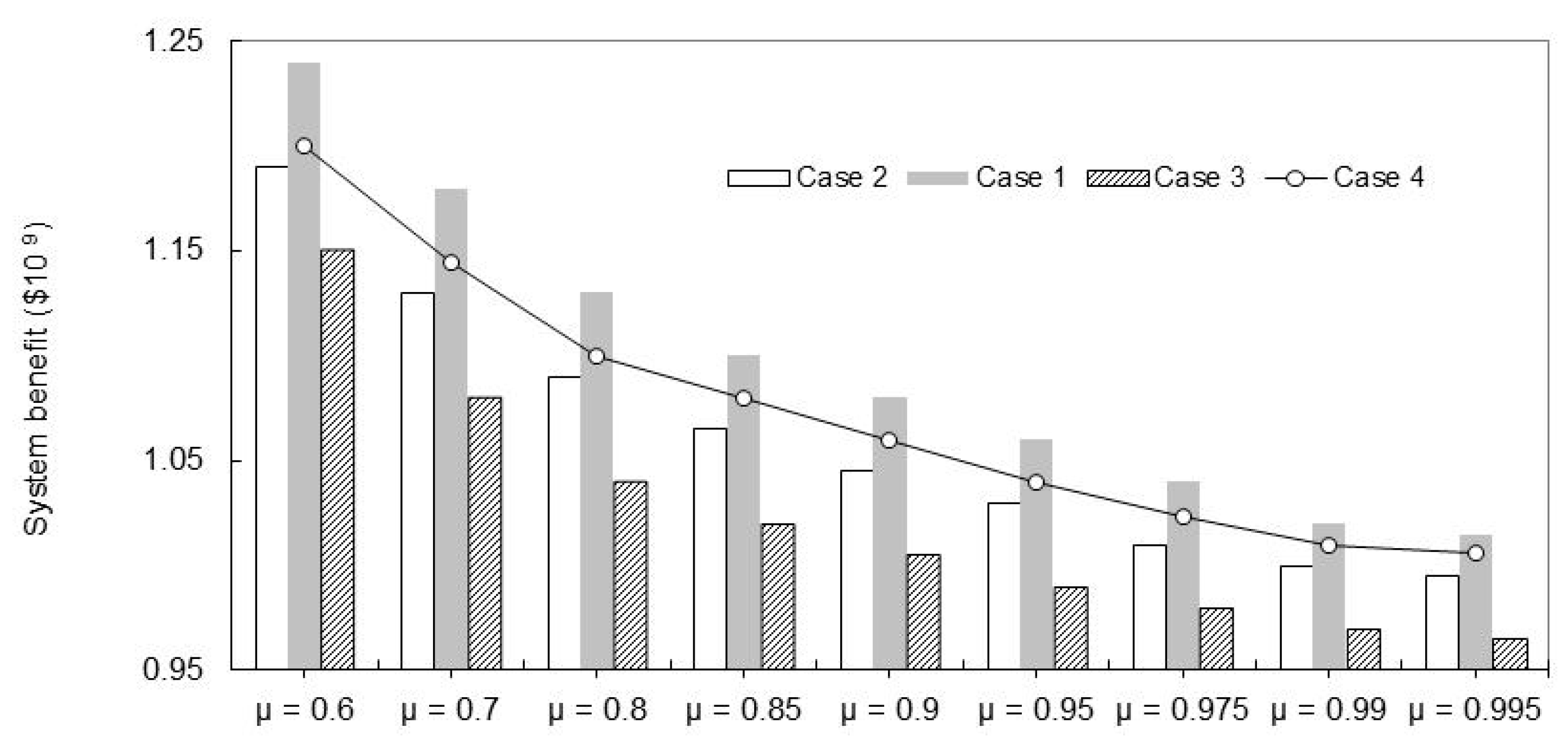
Case 4	Laplace scenario, which is calculated by BS, CS and PS by Laplace’s criterion.

presents four scenarios (i.e., cases 1–4) associated with basic, conservative, progressive and Laplace scenarios, which can reflect the risk attitude to expected water demand target (pre-regulated by policymaker) and actual water usage for agricultural development (for farmer). In Table 3, current water plan deemed as the basic scenario (Case 1), where expected water demand targets would generate the risk of water deficit acted as an actual level. Case 2 is a conservative scenario for a risk-avoiding policymaker, which present a lower expected water demand target for agricultural development. Under random rainfall, a lower risk of water deficit would be obtained to fit for a risk-avoiding policymaker; while, it might generate a higher opportunity cost loss. As we known, in the study region, increasing water demand due to population growth and economic development can excess what natural system can afford, leading to a great risk of water deficit. Case 3 is deemed as a progressive scenario for a risk-seeking policymaker, where the water demand target is increased by the speed of agricultural development. It presents a higher expected water demand target for agricultural development, which would have a higher risk of water deficit. Case 4 is a Laplace scenario for a risk neutral policymaker.

4. Results Analysis

4.1. Soil Loss and Pollution Discharge without Ecological Effect

Figure 2 shows excessive soil loss and TN/TP discharge from crop irrigation without ecological effect under case 1 when µ are 0.6 In Figure 2a1–a3, the results present that the soil loss from crop irrigation with high runoff. The highest values of soil loss occur in grain plant, while the lowest ones can be obtained in vegetable plantation. Due to regional population growth and agricultural development, the irrigative area has been expanded in the future, which result in a greater soil loss. For instance, the soil loss of oil plant would be 369.69, 440.19 and 524.13 × 10³ ton in periods 1, 2, and 3. Figure 2b,c show excessive TN and TP discharges without ecological effect. The remnant of fertilization can be washed into water body with rainfall and soil loss, in which the TN and TP are main sources of pollutant discharges from farming crops. Meanwhile, the results indicate that the excessive TN and TP discharges would change with water flow levels, where higher water flows can generate higher diffusion capacities of pollution, leading lower excess discharges. For example, in period 1, excessive TN discharges of grain plant would be 10.84, 10.58, 9.64, 9.19, and 8.91 × 10³ ton when water levels are low, low-medium, medium, medium-high, and high levels under case 1 when µ are 0.6. Moreover, the results indicated that tight allowance discharge can lead a higher excess discharge, which result in economic penalty due to violating water quality requirement. Under these situations, policymakers should adjust pollutant regulation strategy based on the risk levels.

4.2. Water Deficit without Ecological Effect

Figure 3 presents the water deficit without ecological effect under case 1 when µ are 0.6, 0.8, and 0.99. Results demonstrate that probabilistic water deficit would occur if the pre-regulated target cannot be met, which can be caused by random water flow. Meanwhile, since approximate 60% of the actual precipitation falls concentrate on wet season (from June to September), when inflows are middle or low, the water deficit would be fortified. In comparison among agricultural activities and forest protection, the crop irrigation considered as the biggest water consumer would be confronting severe water deficit. On the contrary, the expected targets of farmer living would be satisfied in response to the drinking water safety. For instance, under case 1, when inflow is medium in period 2, water deficits of crop irrigation, livestock production, and forest protection would be 0.18, 1.45, 0.61, and 0.23 × 10⁶ m³. Moreover, the results present that water deficits would vary with µ-levels. The lower µ levels (i.e., µ = 0.6) would result in higher water deficit; vice versa. For example, when water availability is low in period, water deficit of economic forest would be from 3.16 to 3.72 × 10⁶ m³ when µ levels are from 0.6 to 0.99.

4.3. Ecological Effects and Corresponding Benefits

In the study region, an agroforest ecosystem (AEP) would be established based on integrating agricultural activities (including farmer living, crop irrigation, and livestock production) and forest protection into a framework, which can formulate an effective system to exertion of ecological functions. Figure 4 present the ecological effect under case 1 when µ levels are varied. The results indicate the forest system (including economic forest, shelter forest, and forest park) has played important roles in soil intention, water conversation, and pollution purification, leading to economic returns to human activities. Among them, shelter forest has a higher contribution to soil loss intension; meanwhile, the forest park has played an important role in water conversation. Besides, the results indicate that the ecological function would change with η levels. For instance, the highest µ level (µ = 0.99) would result in lowest ecological effects, which means that higher confidence levels can result in lower ecological effects.

Figure 5 presents ecological benefits from AEP under case 1 when µ level is 0.99. In this study, the ecological benefit can be imposed of direct and indirect benefits. Among them, the direct benefit of AEP would be from withdrawing reclamation, which can reduce penalty of soil loss and pollution discharge. For instance, withdrawing reclamation of grain plant (denoted as GP) would reduce the damage to environment, which would bring about 49.6% of the direct benefit at highest.

The indirect benefit would be from the improvement of ecological function (e.g., improvement of water quality and elevation of water/soil conservation) due to forest recovery. For example, in period 3, forest park can bring about highest indirect benefits from water conservation, which is achieving 46.7% of the total benefits.

4.4. Optimal Water Plan with Ecological Effect

Figure 6 presents that the optimal water allocations between crop and forest under cases when µ level is 0.99. The results demonstrate that the optimal water allocation would vary with different cases. The lowest targets are acquired in case 3 (i.e., conservative scenario) in response to its lower expected target values, which can bring about lowest water deficit and allocations. On the contrary, the highest water deficit and allocations would occur in case 2 (i.e., progressive scenario). The values of water deficits and allocations under case 1 (i.e., basic scenario) is in the middle of cases 2 and 3 approximately. However, the smallest differences between expected target and water allocation would generate reliable and rational results under case 4 (i.e., Laplace scenario) with overall consideration of above three cased (cases 1, 2, and 3).

4.5. System Benefit

Figure 7 presents system benefits under various cases when µ levels are varied. Under case 1, the system benefit would drop from $1.24 × 10⁹ to $1.01 × 10⁹, with increment of µ-level (from 0.60 to 0.995), correspondingly. The results implied that the high µ-level and increasing uncertainty for the imprecise objective would correspond to optimistic attitude on the expected system benefit; vice versa. Meanwhile, the results demonstrate that case 3 (i.e., progressive scenario) corresponding to highest targets of economy development would generate extortionate losses of water deficit and retreatment costs of pollution, leading lower system benefits. On the contrary, case 2 (i.e., conservative scenario) can generate lower losses of water deficit and costs of retreatment, but bring about higher expected values and higher opportunity costs, thus also leading lower system benefits. Case 1 (i.e., BS) can produce a middle value between cases 2 and 3. For instance, when µ-level is 0.6, system benefit would be $1.12 × 10⁹ under case 1, which is a middle value between case 2 ($1.14 × 10⁹) and case 3 ($1.05 × 10⁹). The highest system benefit would be obtained under case 4 (i.e., Laplace scenario) with overall consideration of all risks of scenarios, which can produce a reliable and optimal results under equal probabilities of policy scenarios occurrence.

5. Conclusions

In this study, a fuzzy stochastic programming with Laplace criterion (FSL) is developed for planning water resources in an AEP issue to regain the regional ecological function under uncertainties. FSL has advantages, as follows: (a) it built a linkage between expected water demand and random water availability, which can deal with stochastic uncertainties expressed as probability distributions; (b) it can quantify fuzziness in the processes of decision-making with credibility measure, which can improve the quality of fuzzy expression; and, (c) it can tackle risk attitude of policymaker with random scenario based on limited data, which can support generating a feasible compromise between risk-seeking and risk-avoiding attitudes.

The proposed model is applied to a real case of AMP in Xixian county, China. Numbers of discoveries have been displayed, as follows: (a) a rational water resources plan can prompt reclamation withdraw, forest recovery and livestock regulation, which can relive contradictions between agricultural activities and forest protection artificially; (b) the tradeoff between the benefits of ecological function and economic development can generate numbers of scenarios that are associated with various ecological effects, which is beneficial to adjust current agriculture-environment policy; and, (c) risk attitudes of policymakers can influence decision making, where optimized water policies that are based on Laplace’s criterions can support alleviating water-supply conflict, controlling water/soil erosion, mitigating water pollution, and improving ecological function. Therefore, many corresponding suggestions for decision maker can be summarized as follows: (a) a proper water plan in AEP associated with forest protection (recovery) even expansion can be advocated, which can reduce the adverse influence from agricultural activities; meanwhile, it can improve regional ecological functions, leading ecological returns; (b) The promotion of AEP issue can be encouraged into local agricultural planning and management, which can not only promote the efficiency of agricultural activities, but also achieve integrity of economic development and environmental protection process; and, (c) consciousness’s of risk should be taken into policy making process, which can fortify the reliability of water plans in AEP.