Heating Impact of a Tropical Reservoir on Downstream Water Temperature: A Case Study of the Jinghong Dam on the Lancang River


Department of Hydraulic Engineering, Tsinghua University, Beijing 100084, China
*
Author to whom correspondence should be addressed.
Water 2018, 10(7), 951; https://doi.org/10.3390/w10070951
Submission received: 1 June 2018
/
Revised: 5 July 2018
/
Accepted: 11 July 2018
/
Published: 17 July 2018
(This article belongs to the Special Issue Adaptive Catchment Management and Reservoir Operation)
Abstract
:Reservoirs change downstream thermal regimes by releasing water of different temperatures to that under natural conditions, which may then alter downstream biodiversity and ecological processes. The hydropower exploitation in the mainstream Lancang-Mekong River has triggered concern for its potential effects on downstream countries, especially the impact of the released cold water on local fishery production. However, it was observed recently that the annual water temperature downstream of the Jinghong Reservoir (near the Chinese border) has increased by 3.0 °C compared to its historical average (1997–2004). In this study, a three-dimensional (3D) model of the Jinghong Reservoir was established to simulate its hydro- and thermodynamics. Results show that: (1) the impoundment of the Jinghong Reservoir contributed about 1.3 °C to the increment of the water temperature; (2) the solar radiation played a much more important role in comparison with atmosphere-water heat exchange in changing water temperatures; and (3) the outflow rate also imposed a significant influence on the water temperature by regulating the residence time. After impoundment, the residence time increased from 3 days to 11 days, which means that the duration that the water body can absorb solar radiation has been prolonged. The results explain the heating mechanism of the Jinghong Reservoir brought to downstream water temperatures.
1. Introduction
The riverine environment can be influenced by reservoirs and dams, as well as their operations in many forms, including the changing of riverine thermal regimes and downstream water temperatures [1,2,3]. The health, distribution, and functions of aquatic creatures can be influenced by water temperatures [4,5,6,7], so the extensive construction of dams worldwide has long drawn attention to potential effects of damming on downstream thermal regimes [2,8].
Generally, the impact degree of a dam on downstream thermal regimes is decided by its mode of operation and specific mechanism of water release [9]. Many large dams release water from deep portals which are located under the thermocline, namely the hypolimnetic layer of a reservoir. As a result, the cold water is released to the downstream thermal regimes [2,10,11,12]. This case was rarely reported, but some small dams release water from above the thermocline, namely the epilimnetic layer, so temperatures of the downstream water increase [7].
In addition to annual water temperature, reservoirs also influence seasonal thermal patterns of downstream water. In general, in large reservoirs, the moderate temperatures of downstream water in spring and summer are lower than those in winter when the seasonal fluctuations decrease, while they also display a delay of maxima in comparison with natural rivers [2]. Such phenomena were observed at many dams and reservoirs across the world, such as the Dartmouth Dam on the Mitta Mitta River and Burrendong Dam on the Macquarie River, located in Australia [13,14], the regulated Lyon River located in Scotland [15], and the Hills Creek Dam on the Willamette River, located in America [16].
As the upstream part of the Lancang-Mekong River, the Lancang River is the largest international river in Southern Asia [17]. Since the 1950s, to fully exploit the river’s resources, the Chinese government has come up with proposals concerning damming of mainstreams on the Lancang River [18]. At present, six large dams have been put into operation along the mainstream of the Lancang River. These dams include Nuozhadu, Manwan, Gongguoqiao, Dachaoshan, Xiaowan, and Jianghong dams (ranging from upstream to downstream), wherein the Nuozhadu Reservoir was recently put into operation in 2015 [19]. The cascade of dams is constructed with the primary purpose of hydropower generation. According to the hydropower development plan by Huaneng Lancang River Hydropower Company, the hydropower installed capacity will reach 30.0 GW in the Lancang mainstream by 2020 [19]. Nevertheless, the potential hydrological and environmental effects of reservoir impoundment and water release have drawn more attention to downstream countries [17,20,21,22]. Among these potential effects, altered downstream water temperature has become an important focus as it plays a significant role in influencing the combination of structure, growth, reproduction, distribution, and stream productivity of aquatic organisms [23], in addition to which fish in freshwater serve as the major protein source for local animals which live in downstream countries [19]. In view of those deep and large dams located along the Lancang River, the low-temperature outflow has drawn major concern. In addition, the Nuozhadu Dam is equipped with a multi-level stop log door so as to moderate the downstream water temperature to a pre-dam level [24]. Nevertheless, after the impoundment of six large reservoirs, the water temperatures downstream of the Jinghong Reservoir (the most downstream one of the cascade dams) increased, rather than decreased, in all seasons, which is against what has been observed in other large dams. In other words, the upstream multi-level intake structures could probably be unnecessary. As numerical modeling is a powerful and useful tool, we applied it in investigating the reasons why the Jinghong Reservoir had a unique heating impact on downstream water.
Some one-dimensional (1D) models are applicable to simulate the vertical distribution of the water temperature and chemical/biological materials in a lake or reservoir through time [25]. In general, these models are established under the one-dimensional assumption. Specifically speaking, variations in the lateral directions are relatively small in comparison with those in the vertical directions [26] and are widely used because they are fast enough to facilitate long-term simulation and have performed well in simulating the seasonal and inter-annual variations of lake water temperatures [27]. These models include the bulk model of Kraus and Turner [28], DYRESM [29], PROBE [30], the Hostetler Model [31,32], SEEMOD [33], LIMNMOD [34], MASAS and CHEMSEE [35], Minlake [36], GOTM [37], SIMSTRAT [38], LAKE [39,40], CLM4-LISSS [41], and WRF-Lake [42].
Although 1D lake models are more efficient in computation, under certain conditions (such as long, deep reservoirs) water mass exchange in both vertical and longitudinal directions and temperature gradients may be important [25]. Thus, many two-dimensional (2D) models have been developed through the integration of the reservoir, with the aim to reach the motion equations with lateral averaging [43]. Laterally averaged 2D models are applicable to modeling of long and relatively narrow reservoirs with no or negligible lateral inflow or outflows. These models include the model of Box Exchange Transport Temperature and Ecology of Reservoirs (BETTER) [44]; the Computation of Reservoir Stratification (COORS) model [45]; the Laterally Averaged Reservoir Model (LARM) [46]; the model of Generalized Longitudinal-Vertical Hydrodynamics and Transport (GLVHT) [47], which was developed from LARM; the CE-QUAL-W2 developed through GLVHT expansion to include water quality constituents [48]; the Laterally-Averaged Hydrodynamics Model (LAHM) [43]; and the MIKE21 Flow Model, developed by Danish Hydraulic Institute (DHI) Water and Environment [49,50,51,52], which is widely applied. In addition to the laterally-averaged models, vertically-averaged 2D models are also applied when vertical flow variations are not as important as the lateral case, e.g., when the water is shallow [53,54,55]. These models include the North Sea Model [56], the Tokyo Bay Model [57], the Haringvliet Model, and the depth-averaged mathematical model developed by McGuirk and Rodi [55].
Despite the extensive use of 1D and 2D models, the limit in one-dimensional or vertical and lateral averaging has long been realized and the needs for 3D modeling of lakes and reservoirs have raised more discussion [58,59,60,61]. In the past decades, the complex water quality models and 3D hydrodynamic models have been developed thanks to the high-performing super computers at a reasonable cost, as well as the efficient numerical algorithms [62]. The mentioned models include the Curvilinear-grid Hydrodynamics model in three dimensions (CH3D) [63], the Estuarine, Coastal, and Ocean Model (ECOM) [64]; the Environmental Fluid Dynamics Code (EFDC) [65]; the CE-QUAL-ICM model [66]; the model of Water Quality Analysis Simulation Program (WASP) [67]; the Delft3D-FLOW model [68]; the Row-Column AESOP (RCA) model [69]; and the MIKE 3 model by DHI Water and Environment [70].
In order to analyze the complex 3D hydrodynamic and thermodynamic processes more deeply, it is necessary to establish 3D models. Nevertheless, researchers have so far rarely established 3D models for simulation of the environmental and thermal results of damming along the Lancang River [19] in view of the high cost of computation and the lack of observational data. Nowadays, with computational resources and enough pre-dam and post-dam measurement data, we are capable of conducting 3D simulations at the Jinghong Reservoir. The Delft3D-FLOW model was selected for the simulations as it has been widely used around the world and evidence proves that it can simulate sediment transport, flows, water quality, waves, morphological developments, and ecological courses in coastal regions, rivers, and lakes [71,72,73,74,75,76,77,78]. After model calibration, the 3D model of the Jinghong Reservoir was used to simulate the thermodynamic and hydrodynamic situations in the reservoir, as well as the related outflow. The research also carried out some numerical experiments to analyze the heating impact brought by the Jinghong Reservoir to downstream water.
2. Study Area
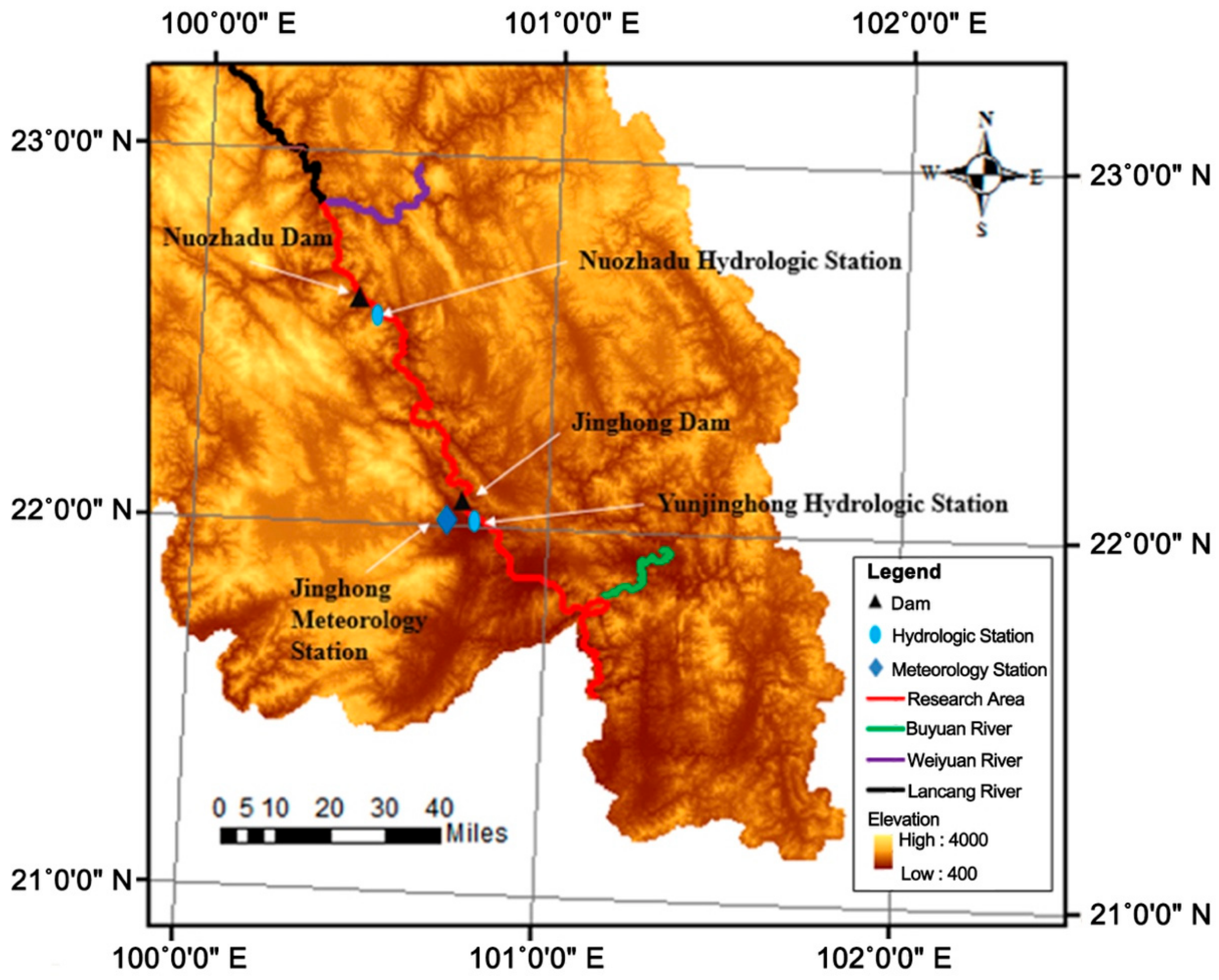
The Jinghong Reservoir system is located in the lower reaches of the Lancang River, which is, in general, a south-flowing river in southwestern China, and called the Mekong River when entering Laos (Figure 1). This system is defined by the Nuozhadu Dam (22°38′ N, 100°26′ E), the Jinghong Dam (22°03′ N, 100°46′ E), and the 105-km long water body between the two (i.e., the Jinghong Reservoir). The Jinghong Dam went into service in 2009 with a height of 108 m, while the Nuozhadu Dam was put into operation in 2015 with a height of 262 m. The Jinghong Reservoir is a long and narrow channel-shaped reservoir with a length of 105 km and an average width of 312 m. It has a normal water level of 602 m above sea level, a maximum depth of 70 m and a total reservoir capacity of 1.14 billion m3. Since the operation of the reservoir, the water surface area has increased from 12.7 km2 to 32.8 km2. The mean annual inflow is about 1674 m3 s−1. A tropical reservoir, the Jinghong Reservoir, has a perennial mean air temperature reaching 22.2 °C at the Jinghong Dam.
2.1. Observation Data
The two hydrological stations involved in the study area are the Nuozhadu Hydrological Station (NHS) and the Yunjinghong Hydrological Station (YHS), both located on the right bank of the river, with the former 5 km downstream of the Nuozhadu Reservoir, and the latter 3 km downstream of the Jinghong Reservoir. Both NHS and YHS are located at the riverine section of the water body, and the fully mixing assumption can be applied. Accordingly, point-measured water temperature can be used as an indicator of the cross-sectional water temperature. To measure the water temperature, water pressure, and air pressure, a Hobo Onset U20-001-02 water level data logger (U20 hereafter) is adopted at each hydrological station on an hourly basis throughout the study period. The water level at each station is computed by:
where (Pa) is the U20-measured pressure underwater (water pressure and air pressure), (Pa) is the U20-measured atmospheric pressure by the river bank, (Pa) is the pressure of pure water, and is the depth of the U20, from which water levels are computed. The discharge at YHS is further computed using its rating curve obtained from the Water Resources Department of Yunnan Province, China [79].
2.2. Observation Data Analysis
2.2.1. Comparison with Historical Water Temperature
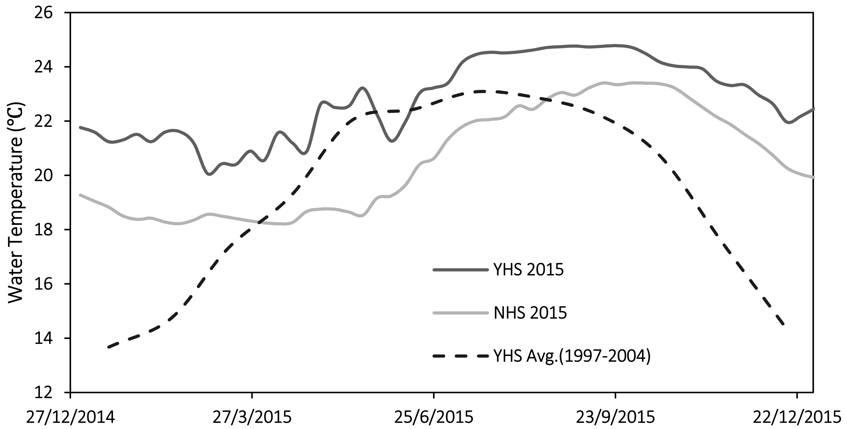
To illustrate the annual variations of water temperature at NHS and the Jinghong Reservoir, in situ observations were conducted (Figure 2). Water temperatures almost changed synchronously at the two sites throughout the year, with NHS always displaying a lower temperature (a mean difference of 2.2 °C) than the other. This systematic temperature difference reflected the latitude difference between the two sites as water flowed south, a phenomenon not observed at reservoirs flowing in other directions. According to a study on the Cougar Reservoir (an eastern-flowing reservoir in the U.S.), the peak of outflow water temperature lagged about 2 months behind that of inflow, but the inflow and outflow temperatures shared the same maximum and minimum values [80], indicating no large amount of energy was taken in, or lost, as the water body flowed into the reservoir.
Obtained and averaged from 1997 to 2004 at YHS, historical water temperature observations (Figure 2) were shown to range between 13.7 and 23.1 °C annually. However, after the impoundment of the Jinghong Reservoir, the water temperature range was changed to between 19.8 and 25.0 °C, with the annual variation reduced from 9.5 °C to 5.2 °C. This reduction in annual variation mainly resulted from a 6.1 °C increase in the minimum temperature. Overall, the annual average water temperature rose from 19.2 °C to 22.8 °C after impoundment.
2.2.2. Discharge and Water Temperature
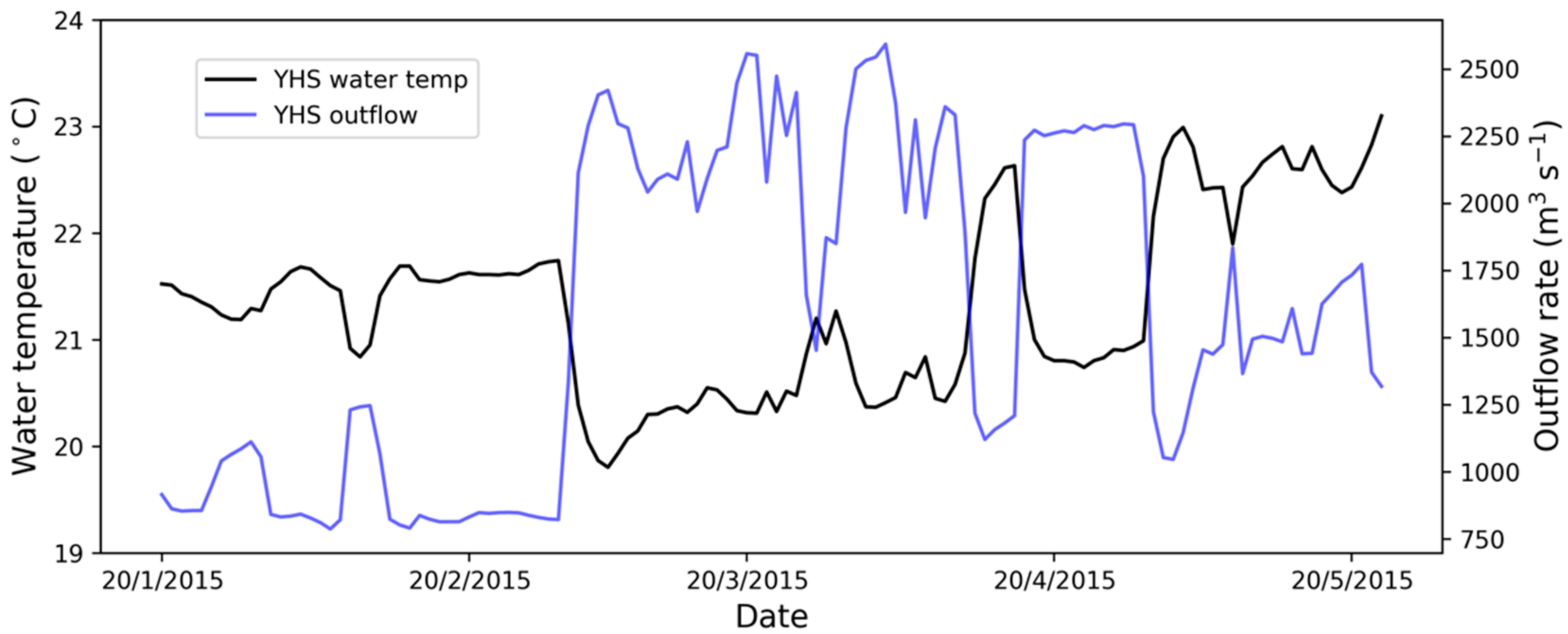
Observed water temperatures at YHS were compared with outflow rates from the reservoir in Figure 3. As they were inversely correlated, the discharge rate of the Jinghong Dam could also be a potential factor behind the water temperature alteration.
3. Methods
3.1. The Delft3D-FLOW Model
The numerical hydrodynamic modeling system—the Delft3D-FLOW model—was developed by Deltares [68], a Dutch-based research institute. The Delft3D-FLOW software used for this study is based on Fortran and acquired from Delft3D website (https://oss.deltares.nl/web/delft3d/). With Delft3D-FLOW, the 2D (based on averaged depth) and 3D shallow water equations that were unsteady could be solved. The equation system comprises momentum equations in the horizontal plane, the continuity equation and the transport equations of conservative elements [68]. The basic equations are retained in their original form and are not changed in this study, which are introduced briefly as follows.
As for the hydrodynamic equations, Delft3D-FLOW is used for the solution of the Navier-Stokes equations with regard to a fluid which is incompressible under the assumption of Boussinesq and the shallow water environment [81]. In the equation of vertical momentum, the accelerations in the vertical direction are omitted, leading to the equation of hydrostatic pressure. Vertical speeds are computed according to the continuity equation in 3D models. The set of partial differential equations, together with a proper set of boundary and initial situations is solved via a mesh with finite differences. Delft3D-FLOW uses orthogonal curvilinear Cartesian coordinates (ξ, η) in the horizontal direction. Two different vertical grid systems are offered by Delft3D-FLOW, vertically: the Cartesian Z coordinate system (Z-model) and the σ coordinate system (σ-model). The σ coordinate system was first introduced by Phillips [82] and it is applied in this research.
To obtain the continuity equation with averaged depth, the continuity equation shall be integrated for incompressible fluids () based on the total depth, wherein the conditions of the kinematic boundary on the bed level and at the water surface are taken into account. It is expressed as follows:
where (m) is the water level on a number of horizontal planes of reference (datum), the coefficients and (m) are used for transformation from curvilinear coordinates to rectangular coordinates, (s) is the time, (m) is the depth under a number of horizontal planes of reference (datum), (m s−1) is the depth-averaged speed in -direction, (m s−1) is the depth-averaged speed in -direction, and (m s−1) is the contributions made for each unit area because of the withdrawal or release of water, evaporation and precipitation.
The momentum equations in -direction and -direction are expressed as follows:
where , , and (m s−1) are speeds in , , and -directions. . (s−1) is the Coriolis parameter (inertial frequency), (kg m−3) is the referential density of water, and (kg m−2 s−2) are the gradient-based hydrostatic pressure in -direction and -direction, and (m s−2) are the imbalances existing in horizontal Reynold’s stresses in the -direction and -direction, (m2 s−1) is the vertical eddy viscosity, and (m s−2) are source or sink of momentum in the -direction and -direction. Reynold’s stresses and are simulated on the basis of the concept of eddy viscosity [83]. The eddy viscosities in vertical and horizontal directions are as follows:
where is the viscosity computed with the 3D k-ε closure scheme, is the user-defined background horizontal viscosity, is the user-defined background vertical viscosity, (m2 s−1) is the kinematic viscosity (molecular) coefficient of water.
Transport of heat and matter is simulated by an equation of advection diffusion in three coordinate directions, and is expressed as follows:
where (kg m−3) is the concentration of mass, (m2 s−1) is the total diffusion coefficient in the horizontal direction, (m2 s−1) is the diffusion coefficient in the vertical direction, (s−1) is the first order decay course and (kg m−2 s−1) is the source and sink terms in the unit area generated from the withdrawal or release of water and/or heat exchange on the free surface. The diffusion coefficient in the horizontal direction is user-specified, whereas the coefficient in the vertical direction is computed as follows:
where is the 2D part of diffusion based on the turbulence model of sub-grid scale, is the user-defined eddy diffusivity in the horizontal direction, is the eddy diffusivity in the vertical direction, is the Prandtl-Schmidt number for molecular mixing, and is the diffusion due to turbulent eddy viscosity [68].
3.2. Model Set-Up
3.2.1. Grid Coverage
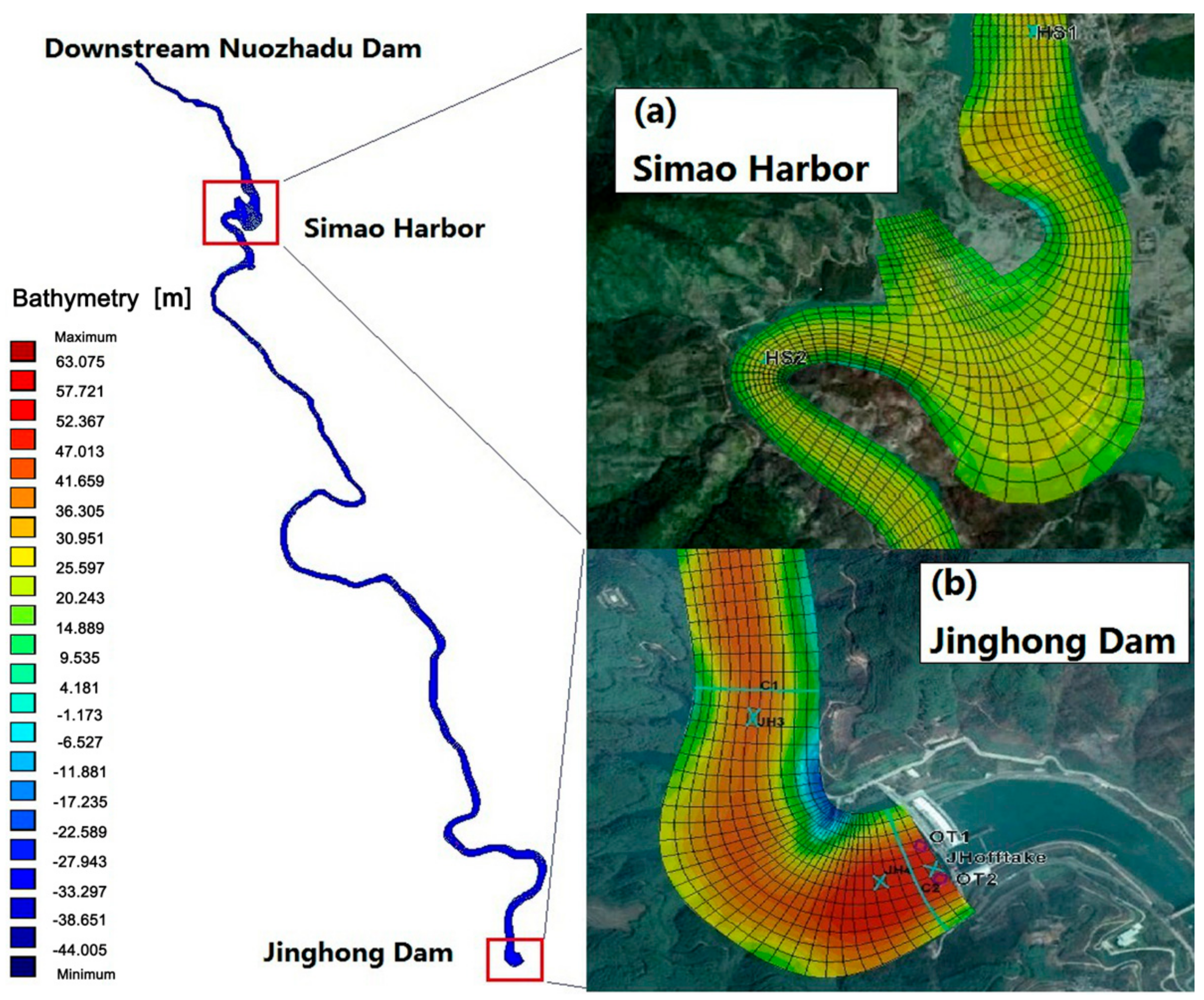
Along the river flow direction, the upper boundary of the model is set to the Nuozhadu Hydrological Station, whereas the lower boundary of the model is set to the Jinghong Dam. With a longitudinal length of about 95 km, the model covers most parts of the Jinghong Reservoir. The computational grid of the Jinghong Reservoir hydrodynamic model is shown in Figure 4. Grid density varies with topography, i.e., in order to increase the computation accuracy, finer horizontal grids have been placed at the part of the reservoir close to the Jinghong Dam, resulting in a total of about 11,000 horizontal grid cells per layer. Meanwhile, for the vertical direction, the σ coordinate system (σ-model) is applied, with the reservoir discretized into 40 vertical layers, with each layer less than 2 m in thickness.
3.2.2. Boundary Conditions
The upper boundary is set at the water level at NHS and the lower boundary is set at the discharge rate downstream of the Jinghong Dam. The terrain data is extracted from a digital elevation model (DEM) with a spatial resolution of 25 m × 25 m.
3.2.3. Meteorological Data and Model Flow Chart
Restrained by the poor data availability, the simulation only covers a period from 20 December 2014 to 22 May 2015. The computational time step is set to 1 minute to meet the demand of numerical stability, as well as computational efficiency.
Meteorological data for this study, which is obtained from the Jinghong National Meteorological Station (Figure 5), is not readily available. As a result, such data is only gathered for a relatively short period, from 20 December 2014 to 20 May 2015, which also defines the study period for this research. These data include local air temperature data, relative humidity data, and solar radiation data with a temporal resolution of 1 day. We acknowledge that it would be better if a full year simulation could be conducted. However, due to solar radiation data availability, 5-month simulation is the best we can practice at the current stage. Similar simulations with temporal coverage of less than 1 year can also be found in the literature [84,85,86].
A flowchart illustrating the Jinghong Reservoir hydrodynamic model is shown in Figure 6.
3.3. Model Calibration and Validation
The warm-up period of this study occurs from 22 December 2014 to 31 January 2015.
For the purpose of verifying the hydro-dynamic condition of this simulation, the simulated water levels were firstly calibrated against measurements. As the model output temporal resolution was 10 minutes, the hourly average for simulated water levels was calculated for comparison. Data on 2 days’ on-site observed water levels at Simao Harbor were provided by field experiment. The best match of the model output and measured data (Figure 7) were achieved by applying critical parameters, as shown in Table 1.
Five main parameters were calibrated by Chanudet et al. (2012): the Chezy’s coefficient, which represents the roughness at the water bottom, background horizontal and vertical eddy viscosity, and background horizontal and vertical eddy diffusivity. The studied range of Chezy’s coefficient can be referred to Chow (1959), while the range of the background eddy viscosity and diffusivity can also be referred to in previous studies [87,88,89].
The focus of the calibration then shifted to outlet water temperatures downstream the Jinghong Dam. As YHS was within 3 km downstream of the Jinghong Reservoir in the riverine section of the water body, the simulated outlet water temperature was compared with the measured water temperature at YHS for calibration, with the difference between the two shown in Figure 8. The simulated results were in good agreement with measurements, with the absolute error limited to 1.5 °C.
Compared with measurements, the Jinghong Reservoir model produced good simulations of water temperatures. Nevertheless, since insufficient observations of the water velocity fields were available, no comparison concerning water velocity was carried out either for calibration or for validation.
3.4. Numerical Scenario Setups
As presented in Section 2.2, three main issues are ought to be found out through numerical modeling: the impact of impoundment of Jinghong Reservoir; the contributing factor to water temperature increment; and the relation between outflow rate and outflow temperature from Jinghong Dam. The wind speed and relative humidity were precluded as the driving forces and several numerical experiments were performed (Table 2).
● Impact of Impoundment of the Jinghong Reservoir
A control run (CTL) was set up as described in Section 3.2 and Section 3.3.
S1 (i.e., scenario 1) was set up to examine the impact of the impoundment of the Jinghong Reservoir, in which the Jinghong Dam was removed and the water body returned to the natural river conditions. A depth-averaged two-dimensional flow model with the same horizontal grid discretization was set up, with the upper boundary condition as described in Section 3.2.2, the Q-H rating-curve adapted as the downstream boundary condition and the atmospheric data as for CTL.
● Contributing Factors
To examine the contribution of solar energy to the increase of water temperatures, S2 was imposed with no solar radiation. To further evaluate the impact of heat exchange with the overlying atmosphere on water temperature, atmosphere-water heat conduction, together with solar radiation was turned down in S3.
● Outflow Rate and Outflow Temperature
Different scenarios were further established so as to investigate the relationship between the outflow rate and the outflow water temperature at the Jinghong Dam. The water temperature measured at YHS was constantly higher than the one measured at NHS, suggesting that the water parcel experienced an energy absorption process travelling from NHS to YHS. In addition to the rate of energy transfer, the amount of energy absorbed by the water parcel was also determined by the duration of the absorption process. The outflow rate directly affected the time during which the water parcel absorbed energy. In order to measure the duration of the energy absorption process, the tracer function of the model was enabled. The duration of energy absorption is represented by the resident time of the tracer. Different scenarios were established to assess the relationship among the outflow rate, resident time, and inflow-outflow temperature difference. In addition, for the sheer size difference between the Nuozhadu Reservoir (upstream) and the Jinghong Reservoir (downstream), the Jinghong Reservoir’s outflow rate was determined by the outflow rate of the Nuozhadu Reservoir. To further simplify the simulation, an assumption was made that the Jinghong Reservoir’s inflow rate is equal its outflow rate. The inflow water temperature at the upper boundary was set to the same as for CTL. The simulation duration remained the same as CTL.
The real outflow rate for the Jinghong Reservoir ranged from 536 to 3398 m3 s−1 and with an annual average of 1674 m3 s−1 in 2015. Eight scenarios were established to examine the effect of outflow rates of the Jinghong Dam, with outflow rates prescribed from 500 to 4000 m3 s−1, with 500 m3 s−1 as intervals. The eight scenarios had been denoted as F1–F8 in the study.
4. Results and Discussion
4.1. Thermal Structure of the Jinghong Reservoir
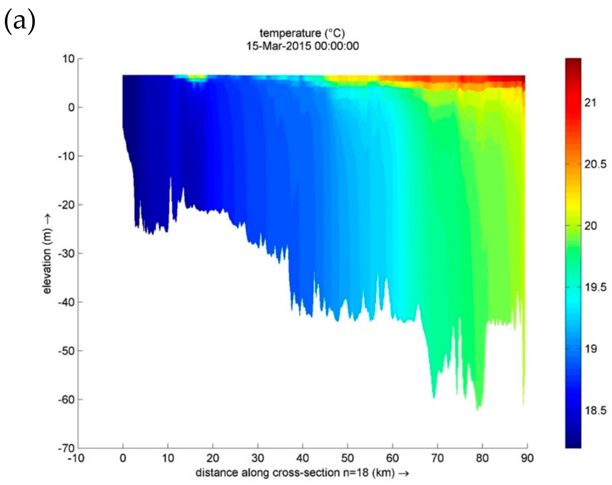
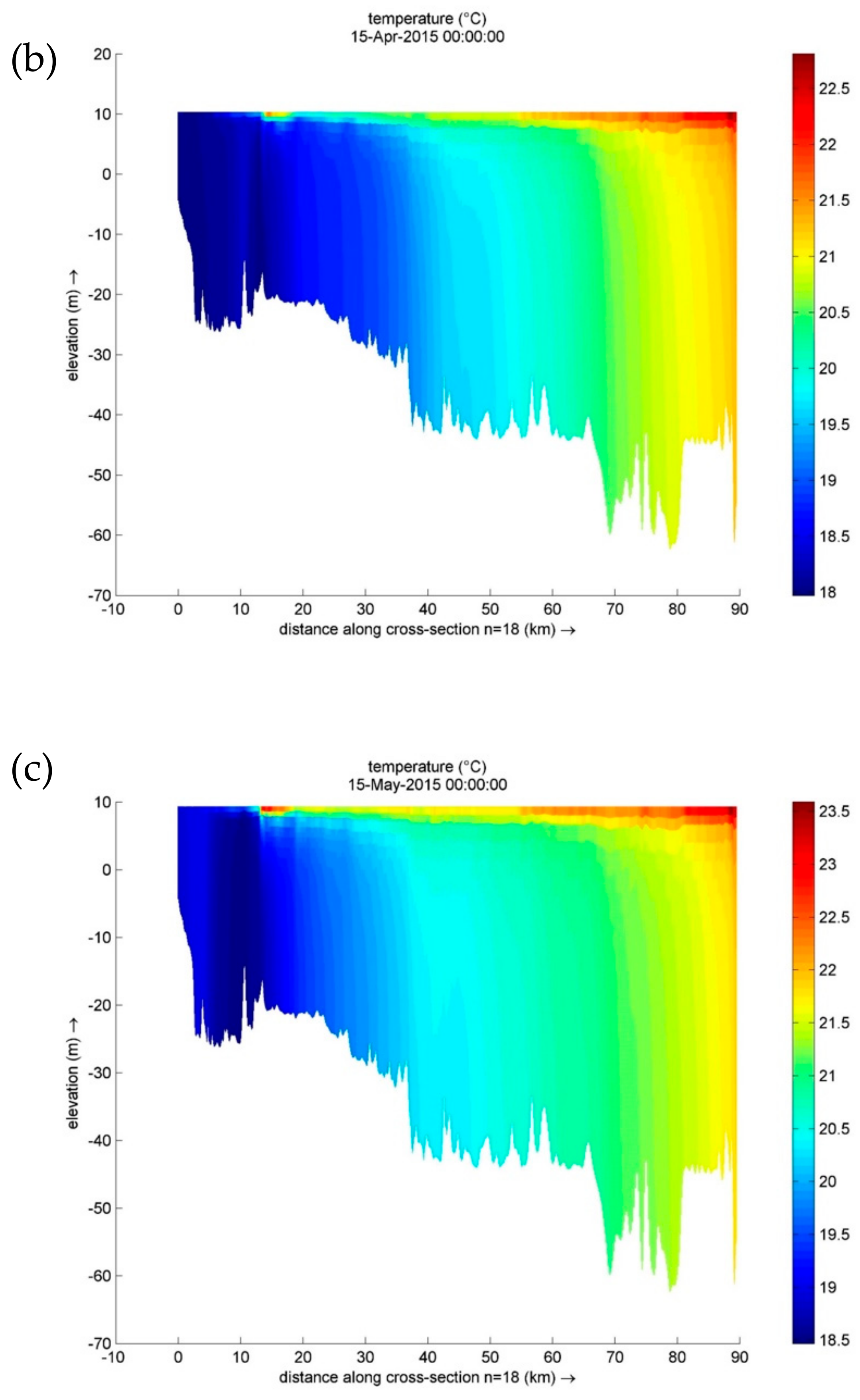
Covering a distance of 105 km, the Jinghong Reservoir has a water depth roughly increasing along the direction of the river flow. The thermal structure along the reservoir from 10 km down the Nuozhadu Dam to the Jinghong Dam (about 90 km) is shown in Figure 9 (3 days corresponding to different months were selected for demonstration). Generally, the water temperature was almost homogeneous during the cool season from December 2014 to February 2015. As the air temperature increased from February on, a warmer water layer appeared at the surface, which eventually developed into a weakly stratified thermocline at the depth of approximately 5 m by the end of May 2015. Unlike many natural lakes, which experienced overturn in early spring, no overturn was observed during the study period at the Jinghong Reservoir, as it was a tropical one and the surface water temperature never went below 4 °C.
During the study period, only weak stratification was observed in the Jinghong Reservoir in May with the surface-bottom temperature difference reaching only 3 °C. In comparison, much stronger stratifications were reported at other deep reservoirs along the Lancang River after impoundment. For example, the Nuozhadu Reservoir (upstream reservoir to the Jinghong Reservoir) experienced a surface-bottom temperature difference of 10 °C in summer and the largest temperature difference in the Xiaowan Reservoir even reached 14 °C [90]. One main reason is the depth difference between these reservoirs. The Jinghong Reservoir is 70 m deep, while the Nuozhadu and Xiaowan Reservoirs are much deeper, each more than 200 m. By preventing solar radiation and wind-driven eddy penetration, large water bodies in these two deep reservoirs retard heat transfer and are difficult to reach a homogeneous temperature. Another reason is the water exchange index, or the α index, which is a widely used approach [91] in identifying reservoir thermal structures, defined by:
where (m3) is average annual inflow and (m3) is the total capacity of the reservoir. When , the reservoir is stably stratified; when , the reservoir is unstably stratified; when , the reservoir is mixed. The α index of the Jinghong Reservoir is much higher compared with that of the other two (Table 3). The large quantity of annual inflow (~ 25 times that of reservoir capacity) serves as a major disturbance, leaving the water body well mixed.
Vertically, the water columns along the reservoir showed almost no stratification regardless of their location and depth. The water temperature difference between surface and bottom was less than 1 °C in the first 40 km along the reservoir in all simulated time, while its maximum of 3 °C was reached at the Jinghong Dam in May. Longitudinally, water surface temperature rose as the river flowed southward, with its value down the Nuozhadu Dam increasing from around 18.5 °C all the way down the river, to approximately 22 °C before the Jinghong Dam. Temporally, water temperature changed in accordance with air temperature. When the air temperature was lower than the water temperature in January and February, the water temperature experienced a drop, while when the air temperature was higher than the water temperature from March to May, the water temperature rose. However, the water temperature variation also increased longitudinally, with the variation down the Nuozhadu Dam being only 0.5 °C and reaching 3 °C at the Jinghong Dam.
4.2. Impact of Solar Radiation and Air Temperature
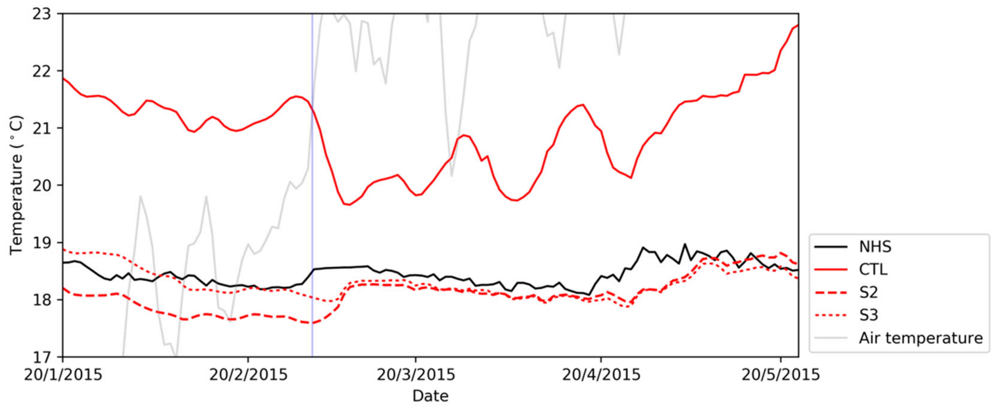
The absorption of solar radiation and atmosphere-water heat conduction are the two main heat exchange mechanisms governing a water body and the environment. Therefore, the contribution to water temperature alteration provided by solar radiation and atmosphere-water heat conduction can be revealed by comparing the model results of S2 and S3. By removing solar radiation, scenario S2, a notable water temperature drop with a mean value of 3 °C compared with CTL (Figure 10) has been observed. In fact, the water temperature simulated by S2 is rather close to the one measured at the NHS with a mean difference of only 0.4 °C. This indicates that the water parcel does not take in or emit substantial energy while traveling from the NHS to YHS. By further neglecting atmosphere-water heat conduction, S3 produces similar water temperature profiles to the ones of S2. The mean simulated temperature in these two scenarios differs about 0.3 °C, which suggests that the solar radiation, rather than the atmosphere-water heat conduction, plays the dominant role in altering water temperature. Moreover, the difference between S2 and S3 (S2 minus S3) varies with season. The difference reached its maximum (about 0.8 °C) in January and February when air temperature was significantly lower than the water temperature, signifying the water energy loss to the atmosphere. However, in May, when air temperature was substantially higher than the water temperature, the difference is positive (about 0.2 °C), indicating the overlying air heats up the water body.
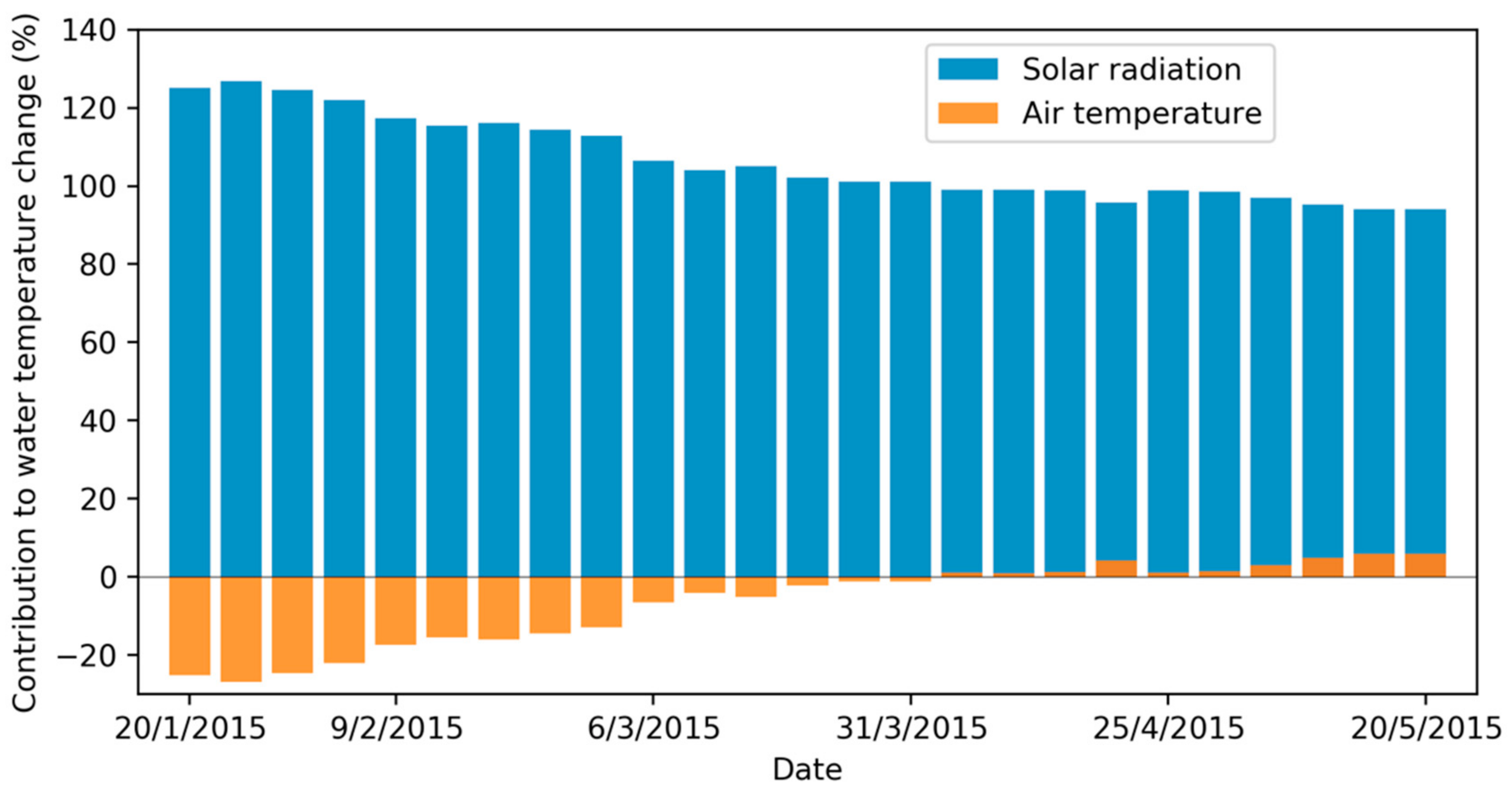
The difference between the simulated water temperature in scenarios CTL and S3 at the YHS was taken as the total impact of solar radiation and air temperature and the weekly contribution (percentage) of both factors were evaluated (Figure 11). Overall, the solar radiation’s contribution to the water temperature increment was 106.7%. However, the contribution of air temperature was −6.7%, which suggests that atmosphere-water heat conduction has a decreasing effect on water temperature during the study period. In addition, it is worth observing that the contribution of air temperature is largely dependent on the air-water temperature difference and may vary with simulation periods. When the air temperature was significantly lower than the reservoir water temperature in January and February 2015 (left side of the vertical blue line in Figure 10), its contribution could reach as much as −24%. When the air temperature approached and eventually exceeded the water temperature, the air temperature’s contribution to the water temperature increment, became more significant.
4.3. Impact of Outflow Rates
A negative correlation between outflow rates and outflow temperature has been observed in Section 2.2.2. For reservoirs with small capacities, a negative relationship between outflow rates and outflow temperature has been reported [92,93]. To further analyze the impact of outflow rates, we carried out eight scenario experiments with different outflow rates ranging from 500 to 4000 m3 s−1.
One and a half period of the tracer concentration has been designed so as to easily differentiate the respective peak concentration value from outflow, which would increase the readability of the residence time. However, the temporal length of the period is not much restrained, as long as it is longer than the longest residence time studied and shorter than the simulation period, it would be sufficient in explaining the problem. Using seven different concentrations instead of a single concentration would also increase the readability. Additionally, under different scenarios, the diffusion effect is also associated with the residence time. By using seven different concentrations, the tracer effect could be observed from both temporal and amplitude points of view.
Outflow rates regulate the residence time of the reservoir. By definition, the residence time refers to how long a parcel, starting from a specific location within a water body, will remain in the water body before exiting [94]. Generally, the residence time decreases as the outflow increases, which results in a shorter duration available for the water parcel to interact with heat sources/sinks (mainly solar radiation and ambient). Thus, its temperature would result closer to the one of the upstream water body. Residence time has been widely used to describe the variability of the lake thermal structure, isotopic composition, alkalinity, dissolved organic carbon concentration, elemental ratios of heavy metals and nutrients, mineralization rates of organic matter, and primary production [95,96,97,98,99,100].
The tracer methodology mentioned in Section 3.4 was applied to measure the residence time in different scenarios. The tracer was released at the Nuozhadu Reservoir with cyclical concentration peaks ranging from 1 to 7 mg m−3 at 1 mg m−3 intervals (Figure 12a). Tracer concentrations at the YHS were recorded. We computed the residence time by:
where is the residence time, is the time of inflow tracer peak of 1 mg m−3, is that of 7 mg m−3, is the time of outflow tracer peak corresponding to and is that corresponding to . When the outflow rate was extremely high at 4000 m3 s−1, the residence time was only about 4 days. On the other hand, when the outflow rate was relatively low at 1000 m3 s−1, it took about 11 days for a water parcel to exit the water body. Generally, the residence time decreased exponentially with the outflow rate and the two variables were highly correlated with a correlation coefficient (R2) of 0.9999 (Figure 12b).
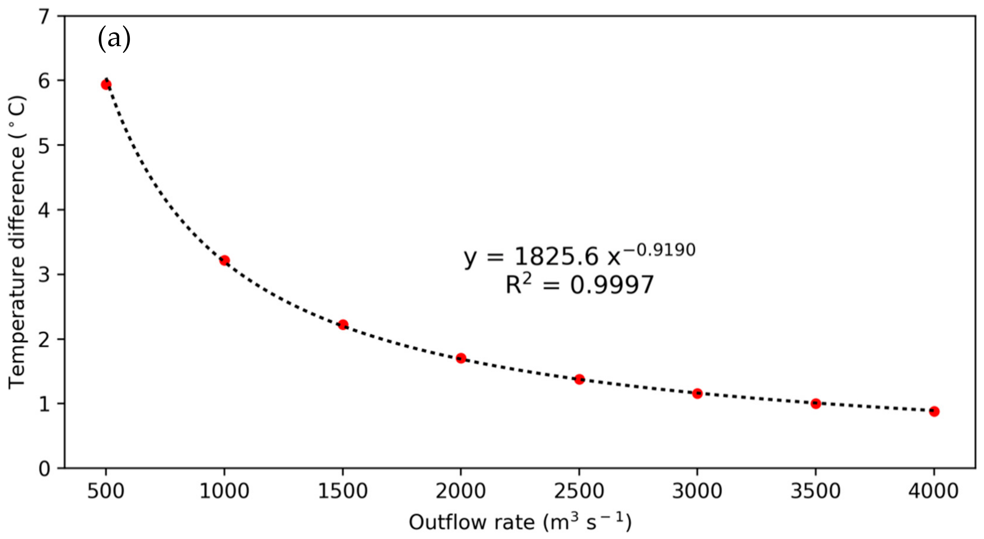
Afterwards, the simulated outflow water temperature at the YHS was averaged during the study period. We used the temperature difference, the averaged outflow temperature minus the averaged inflow temperature, to indicate the temperature changes under different scenarios (F1–F4). Results based on the eight scenario experiments suggested that water temperature difference and outflow rate were also exponentially correlated with an R2 of 0.9997 (Figure 13a). Thus, water temperature difference increased linearly with residence time with an R2 of over 0.9977 (Figure 13b).
To sum up, in the case of the Jinghong Reservoir, outflow rates regulate the residence time. The larger residence time means that the water body is able to absorb more solar energy and, thus, gain a larger temperature increment. Nevertheless, this conclusion is only valid under certain conditions: On one hand, the solar radiation and the atmosphere play a positive role in regulating water temperature; on the other hand, the reservoir capacity is relatively small (for example, the discharge/capacity ratio is larger than 20) so that the outflow rate is able to strongly influence the outflow temperature. The Jinghong Reservoir matches both requirements mentioned above.
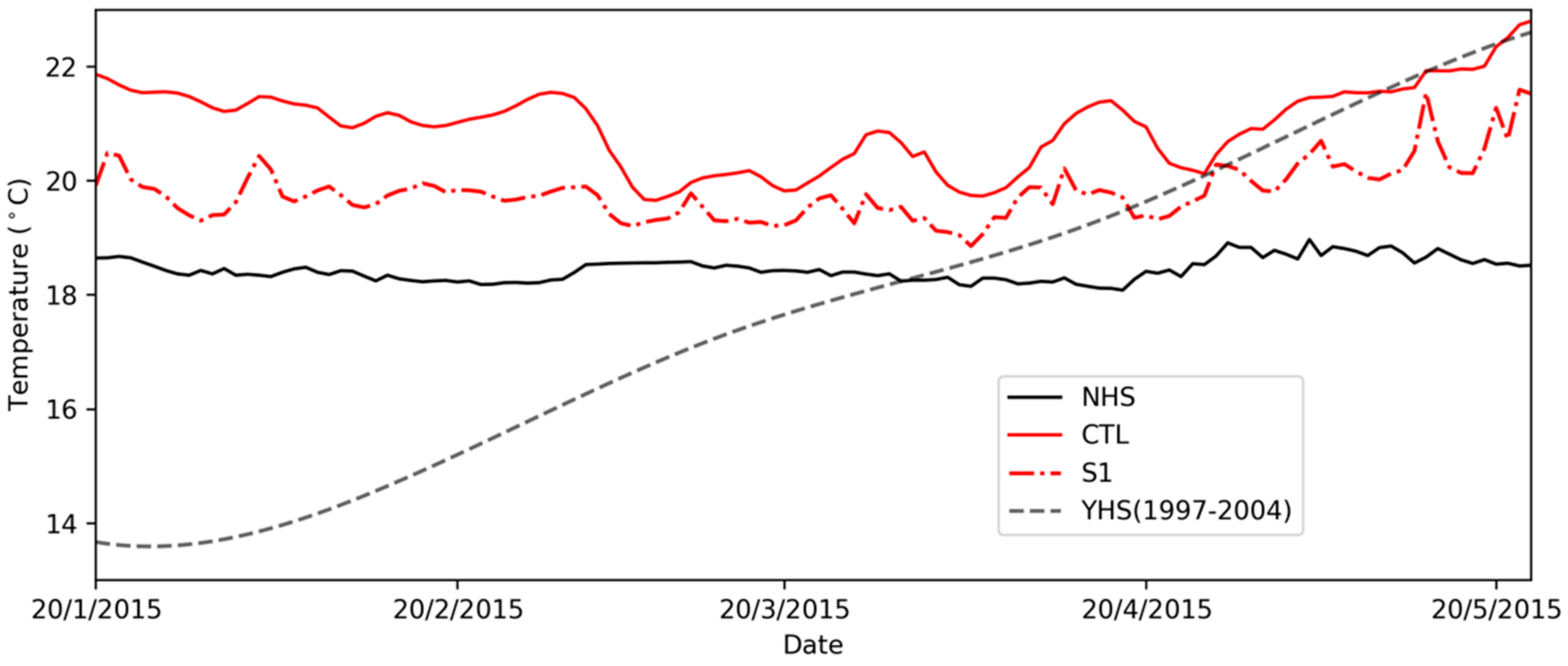
4.4. Impact of the Impoundment
In order to examine the overall impact of the impoundment of the Jinghong Reservoir, we established scenario S1, where the Jinghong Dam was removed and the reservoir recovers to the pre-damming state. During the study period, the water temperature for CTL warmed up by about 3 °C on average. However, when the reservoir returned to the natural river state, the temperature increment was not as significant as for the post-impoundment, with an increment of only 1.7 °C, which was about half the case during the reservoir’s operation (Figure 14). That is to say, the impoundment of the Jinghong Reservoir alone can explain nearly half (1.3 °C) of the water temperature increment from the NHS to the YHS. Based on the findings of Section 4.3, after the impoundment, the residence time extended from 3 days to 11 days. The period available to absorb solar radiation has been prolonged. Thus, a higher water temperature increment is reached.
5. Research Limitations
Though thorough investigation has been conducted, research limitations due to data availability are not ignorable. Firstly, no continuously measured water temperature data on the Lancang River can be found in the previous studies. Therefore, we conducted a field measurement so as to obtain the water temperature information from November 2014 to February 2016. On the other hand, we only obtained daily solar radiation values from January 2014 to May 2015. Therefore, the study period has been greatly shortened. However, the focus of this study is the explanation of the phenomenon, and a study duration shorter than a full year would not undermine its credibility.
In addition, the influence of the operation rules of the dam have not been directly assessed in this research. In this study, the operation rules have been lumped inside the outflow rate, which is only juxtaposed with outflow water temperature so as to indicate the relation among the two. In which way the operation rules would be most favorable to the downstream environment will be another direction of study in our future research.
6. Conclusions
The temperature characteristics of a river are important due to their strong influence on environmental conditions and aquatic creatures. The impact of reservoirs on downstream water temperature has triggered researchers’ concerns worldwide as reservoirs usually release water from deep outlets, in most cases, resulting in a cold water thermal regime downstream. However, the water temperature downstream of the Jinghong Reservoir has increased by 3.0 °C annually compared with historical conditions, according to the observational data. In this study, a Jinghong Reservoir 3D model was established using the Delft3D-FLOW model to explore the unique heating processes of the Jinghong Reservoir on water temperature.
The simulated water temperatures at the outlet showed good agreement with measurements at the Jinghong dam. Comparing the actual operation scenario (CTL) with the pre-damming scenario (S1), it was indicated that the impoundment of the Jinghong Reservoir could explain 1.3 °C (about a half) of the water temperature increase compared to historical values, while the rest might be an accumulated effect by the impoundment of the upstream cascade reservoirs.
Further, this study examined the major factors (solar radiation, atmosphere-water heat conduction) which can potentially influence the water temperature. Numerical experiment results show the contribution of solar radiation to the water temperature increment is up to 106.7%, which consists in the dominating factor. On the other hand, the contribution of the air temperature to the water temperature increment is about −6.7%, which implies that the atmosphere-water heat conduction would result in a decrease of the water temperature during the study period.
Experiment results with different outflow rates (F1–F8) showed that the outflow rate could substantially influence the outflow water temperature because of the variations in the residence time. The residence time is determined by the outflow rate; higher residence time means that the water body absorbs more solar energy and results in a larger temperature increment. After the impoundment of the Jinghong Reservoir, the residence time extended from 3 days to 11 days. The prolonged solar radiation absorption duration is the main reason for its temperature raise.
In conclusion, the Jinghong Reservoir alone could not fully explain the temperature increases compared to historical data since this is also dependent on the accumulated effect by the cascade of dams along the mainstream Lancang River. In the future, a model of the entire cascade of reservoirs should be implemented, in order to improve the assessments of water temperature in pre-dam and post-dam eras.
Author Contributions
Conceptualization: B.J. and G.N.; methodology, validation, and software: B.J.; investigation: F.W. and B.J.; writing—original draft preparation: F.W.; writing—review and editing: B.J., G.N., and F.W.; visualization: F.W.; supervision: G.N.; and funding acquisition: G.N.
Funding
This research was funded by the Ministry of Science and Technology of the People’s Republic of China grant number [2016YFA0601603].
Acknowledgments
We would like to thank Daming He and Ying Lu of Yunnan University for their contribution in collecting water temperature data. Also, we would like to express sincere thanks to the editor and the three anonymous reviewers whose comments led to great improvement of this paper.
Conflicts of Interest
The authors declare no conflict of interest.
References
- Carron, J.C.; Rajaram, H. Impact of variable reservoir releases on management of downstream water temperatures. Water Resour. Res. 2001, 37, 1733–1744. [Google Scholar] [CrossRef]
- Olden, J.D.; Naiman, R.J. Incorporating thermal regimes into environmental flows assessments: Modifying dam operations to restore freshwater ecosystem integrity. Freshw. Biol. 2010, 55, 86–107. [Google Scholar] [CrossRef]
- Rheinheimer, D.E.; Null, S.E.; Lund, J.R. Optimizing selective withdrawal from reservoirs to manage downstream temperatures with climate warming. J. Water Resour. Plan. Manag. 2015, 141, 04014063. [Google Scholar] [CrossRef]
- Hynes, H.B.N. Lotic biology. (Book reviews: The ecology of running waters). Science 1971, 172, 251. [Google Scholar]
- Sullivan, K.; Martin, D.J.; Cardwell, R.D.; Inc, P.; Toll, J.E.; Inc, P.; Duke, S. An analysis of the effects of temperature on salmonids of the pacific northwest with implications for selecting temperature criteria. Sustainable ecosystems institute. Histochemistry 2000, 90, 85–97. [Google Scholar]
- Poole, G.C.; Berman, C.H. An ecological perspective on in-stream temperature: Natural heat dynamics and mechanisms of human-caused thermal degradation. Environ. Manag. 2001, 27, 787–802. [Google Scholar] [CrossRef]
- Lessard, J.A.L.; Hayes, D.B. Effects of elevated water temperature on fish and macroinvertebrate communities below small dams. River Res. Appl. 2010, 19, 721–732. [Google Scholar] [CrossRef]
- Murchie, K.J.; Hair, K.P.E.; Pullen, C.E.; Redpath, T.D.; Stephens, H.R.; Cooke, S.J. Fish response to modified flow regimes in regulated rivers: Research methods, effects and opportunities. River Res. Appl. 2008, 24, 197–217. [Google Scholar] [CrossRef]
- Ward, J.V. Thermal characteristics of running waters. Hydrobiologia 1985, 125, 31–46. [Google Scholar] [CrossRef]
- Brooker, M.P. The impact of impoundments on the downstream fisheries and general ecology of rivers. Adv. Appl. Boil. 1981, 6, 91–152. [Google Scholar]
- Horne, B.D.; Rutherford, E.S.; Wehrly, K.E. Simulating effects of hydro-dam alteration on thermal regime and wild steelhead recruitment in a stable-flow lake michigan tributary. River Res. Appl. 2004, 20, 185–203. [Google Scholar] [CrossRef]
- Krause, C.W.; Newcomb, T.J.; Orth, D.J. Thermal habitat assessment of alternative flow scenarios in a tailwater fishery. River Res. Appl. 2005, 21, 581–593. [Google Scholar] [CrossRef]
- Ryan, T.F.; Webb, J.A.; Lennie, R.; Lyon, J. Satus of Cold Water Releases from Victorian Dam; Dept. of Natural Resources and Environment: Heidelberg, Australia, 2001. [Google Scholar]
- Preece, R. Cold Water Pollution below Dams in New South Wales: A Desktop Assessment; Water management Division, Dept. of Infrastructure, Planning and Natural Resources: Sydney, Australia, 2004. [Google Scholar]
- Jackson, H.M.; Gibbins, C.N.; Soulsby, C. Role of discharge and temperature variation in determining invertebrate community structure in a regulated river. River Res. Appl. 2007, 23, 651–669. [Google Scholar] [CrossRef]
- Angilletta, M.J.; Steel, E.A.; Bartz, K.K.; Kingsolver, J.G.; Scheuerell, M.D.; Beckman, B.R.; Crozier, L.G. Big dams and salmon evolution: Changes in thermal regimes and their potential evolutionary consequences. Evol. Appl. 2008, 1, 286–299. [Google Scholar] [CrossRef] [PubMed]
- Campbell, I.C. The Mekong: Biophysical Environment of an International River Basin; Elsevier Academic Press: Amsterdam, The Netherlands, 2009. [Google Scholar]
- Zhao, A.G. Planning and development of lower and middle Lancang River’s water power resources. Pearl River 2000, 21, 5–8. [Google Scholar]
- Fan, H.; He, D.; Wang, H. Environmental consequences of damming the mainstream Lancang-Mekong River: A review. Earth-Sci. Rev. 2015, 146, 77–91. [Google Scholar] [CrossRef]
- Lu, X.X.; Siew, R.Y. Water discharge and sediment flux changes over the past decades in the lower Mekong River: Possible impacts of the Chinese dams. Hydrol. Earth Syst. Sci. 2006, 10, 181–195. [Google Scholar] [CrossRef]
- Campbell, I.C. Perceptions, data, and river management: Lessons from the Mekong River. Water Resour. Res. 2007, 43, 329–335. [Google Scholar] [CrossRef]
- Lu, X.X.; Li, S.; Kummu, M.; Padawangi, R.; Wang, J.J. Observed changes in the water flow at Chiang Saen in the lower Mekong: Impacts of Chinese dams? Quat. Int. 2014, 336, 145–157. [Google Scholar] [CrossRef]
- Haxton, T.J.; Findlay, C.S. Meta-analysis of the impacts of water management on aquatic communities. J. Can. Sci. Halieutiques Aquat. 2008, 65, 437–447. [Google Scholar] [CrossRef]
- Gao, X.; Zhang, S.; Zhang, C. 3-D numerical simulation of water temperature released from the multi-level intake of Nuozhadu hydropower station. J. Hydroelectr. Eng. 2012, 31, 195–201+207. [Google Scholar]
- Wurbs. Computer Models for Water Resources Planning and Management; S Army Corps of Engineers, Institute for Water Resources: Alexandria, VA, USA, 1994. [Google Scholar]
- Imteaz, M.A.; Asaeda, T.; Lockington, D.A. Modelling the effects of inflow parameters on lake water quality. Environ. Model. Assess. 2003, 8, 63–70. [Google Scholar] [CrossRef]
- Peeters, F.; Livingstone, D.M.; Goudsmit, G.; Kipfer, R.; Forster, R. Modeling 50 years of historical temperature profiles in a large central European lake. Limnol. Ocean. 2002, 47, 186–197. [Google Scholar] [CrossRef] [Green Version]
- Kraus, E.B.; Turner, J.S. A one-dimensional model of the seasonal thermocline II. The general theory and its consequences. Tellus 1967, 19, 98–106. [Google Scholar] [CrossRef]
- Imberger, J.; Patterson, J.; Hebbert, B.; Loh, I. Dynamics of reservoir of medium size. J. Hydraul. Div. 1978, 104, 725–743. [Google Scholar]
- Svensson, U. A Mathematical Model of the Seasonal Thermocline. Ph.D. Thesis, University of Lund, Lund, Sweden, 1978. [Google Scholar]
- Hostetler, S.W.; Bartlein, P.J. Simulation of lake evaporation with application to modeling lake level variations of Harney-Malheur Lake, oregon. Water Resour. Res. 1990, 26, 2603–2612. [Google Scholar]
- Hostetler, S.W.; Giorgi, F.; Bates, G.T.; Bartlein, P.J. Lake-atmosphere feedbacks associated with paleolakes Bonneville and Lahontan. Science 1994, 263, 665. [Google Scholar] [CrossRef] [PubMed]
- Zamboni, F.; Barbieri, A.; Polli, B.; Salvadè, G.; Simona, M. The dynamic model seemod applied to the Southern Basin of Lake Lugano. Aquat. Sci. 1992, 54, 367–380. [Google Scholar] [CrossRef]
- Karagounis, I.; Trösch, J.; Zamboni, F. A coupled physical-biochemical lake model for forecasting water quality. Aquat. Sci. 1993, 55, 87–102. [Google Scholar] [CrossRef]
- Ulrich, M. Modeling of Chemicals in Lakes-Development and Application of User-Friendly Simulation Software (MASAS & CHEMSEE) on Personal Computers. Ph.D. Thesis, Swiss Federal Institute of Technology, Zürich, Switzerland, 1991. [Google Scholar]
- Fang, X.; Stefan, H.G. Long-term lake water temperature and ice cover simulations/measurements. Cold Reg. Sci. Technol. 1996, 24, 289–304. [Google Scholar] [CrossRef]
- Burchard, H.; Bolding, K.; Villarreal, M.R. GOTM, a General Ocean Turbulence Model: Theory, Implementation and Test Cases; Space Applications Institute: Ispra, Italy, 1999. [Google Scholar]
- Goudsmit, G.H.; Burchard, H.; Peeters, F.; Wüest, A. Application of k-ϵ turbulence models to enclosed basins: The role of internal seiches. J. Geophys. Res. Ocean. 2002, 107, C12. [Google Scholar] [CrossRef]
- Stepanenko, V.M.; Lykossov, V.N. Numerical modeling of heat and moisture transfer processes in a system lake—Soil. Russ. J. Meteorol. Hydrol. 2005, 3, 95–104. [Google Scholar]
- Stepanenko, V.M.; Machul’Skaya, E.E.; Glagolev, M.V.; Lykossov, V.N. Numerical modeling of methane emissions from lakes in the permafrost zone. Izv. Atmos. Ocean. Phys. 2011, 47, 252–264. [Google Scholar] [CrossRef]
- Subin, Z.M.; Riley, W.J.; Mironov, D. An improved lake model for climate simulations: Model structure, evaluation, and sensitivity analyses in CESM1. J. Adv. Model. Earth Syst. 2012, 4, 1. [Google Scholar] [CrossRef]
- Gu, H.; Jin, J.; Wu, Y.; Ek, M.B.; Subin, Z.M. Calibration and validation of lake surface temperature simulations with the coupled WRF-lake model. Clim. Chang. 2015, 129, 471–483. [Google Scholar] [CrossRef]
- Karpik, S.R.; Raithby, G.D. Laterally averaged hydrodynamics model for reservoir predictions. J. Hydraul. Eng. 1990, 116, 783–798. [Google Scholar] [CrossRef]
- Brown, R.T. BETTER, A Two-Dimensional Reservoir Water Quality Model: Model User’s Guide; Tennessee Technological University: Cookeville, TN, USA, 1985. [Google Scholar]
- Waldrop, W.R.; Ungate, C.D.; Harper, W.L. Computer Simulation of Hydrodynamics and Temperatures of Tellico Reservoir; TVA Water Systems Development Branch: Norris, TN, USA, 1980. [Google Scholar]
- Edinger, J.E.; Buchak, E.M. Developments in LARM2: A Longitudinal-Vertical, Time-Varying Hydrodynamic Reservoir Model; US Army Engineer Waterways Experimental Station: Visburg, MS, USA, 1983. [Google Scholar]
- Buchak, E.M.; Edinger, J.E. Generalized Longitudinal-Vertical Hydrodynamics and Transport: Development, Programming and Application; US Army Engineer Waterways Experimental Station: Visburg, MS, USA, 1984. [Google Scholar]
- Cole, T.M.; Buchak, E.M. CE-QUAL-W2: A Two-Dimensional, Laterally Averaged, Hydrodynamic and Water Quality Model, Version 2.0. User Manual; US Army Engineer Waterways Experimental Station: Visburg, MS, USA, 1995. [Google Scholar]
- Chen, X.F.; Wang, G.X. Mike 21 software and its application on the offshore reconstruction engineering of Changxing Islands. J. Dalian Univ. 2007, 28, 93–98. (In Chinese) [Google Scholar]
- Wang, Z. Application of Mike 21 in ecological design of artificial lake. Water Res. Power 2008, 26, 124–127. (In Chinese) [Google Scholar]
- Cheng, Y.U.; Ren, X.; Ban, X.A.; Yun, D.U. Application of two-dimensional water quality model in the project of the water diversion in East Lake, Wuhan. J. Lake Sci. 2012, 24, 43–50. [Google Scholar] [CrossRef]
- Liang, Y.; Yin, J.; Zhu, X.; Huang, X. Application of Mike 21 hydrodynamic model in water level simulation of Hongze Lake. Water Res. Power 2013, 31, 135–137. [Google Scholar]
- Leendertse, J.J. Aspects of a Computational Model for Long-Period Water-Wave Propagation; Rand Corporation: Santa Monica, LA, USA, 1967. [Google Scholar]
- Kuipers, J.; Vreugdeuhil, C.B. Calculations of Two-Dimensional Horizontal Flow; Delft Hydraulics Laboratory Report: Delft, The Netherlands, 1973. [Google Scholar]
- McGuirk, J.J.; Rodi, W. A depth-averaged mathematical model for the near field of side discharges into open-channel flow. J. Fluid Mech. 1978, 86, 761–781. [Google Scholar] [CrossRef]
- Lauwerier, H.A. Some recent work of the Amsterdam Mathematical Centre on the hydrodynamics of the North Sea. Sticht. Math. Cent. Toegep. Wiskund. 1961, 1, 1–12. [Google Scholar]
- Isozaki, I.; Unoki, S. The numerical computation of the Tsunami in Tokyo Bay caused by the Chilean Earthquake in May 1960. In Studies on Oceanography—A Collection of Papers Dedicated to Koji Hidaka; Tokyo University Press: Tokyo, Japan, 1964. [Google Scholar]
- Ziegler, C.K.; Nisbet, B. Fine-Grained Sediment Transport in Pawtuxet River, Rhode Island. J. Hydraul. Eng. 1994, 120, 561–576. [Google Scholar] [CrossRef]
- Ziegler, C.K.; Nisbet, B.S. Long-Term Simulation of Fine-Grained Sediment Transport in Large Reservoir. J. Hydraul. Eng. 1995, 121, 773–781. [Google Scholar] [CrossRef]
- Chung, S.; Gu, R. Two-Dimensional Simulations of Contaminant Currents in Stratified Reservoir. J. Hydraul. Eng. 1998, 124, 704–711. [Google Scholar] [CrossRef]
- Tufford, D.L.; Mckellar, H.N. Spatial and temporal hydrodynamic and water quality modeling analysis of a large reservoir on the South Carolina (U.S.) coastal plain. Ecol. Model. 1999, 114, 137–173. [Google Scholar] [CrossRef]
- Ji, Z.G. Hydrodynamics and Water Quality: Modeling Rivers, Lakes, and Estuaries; John Wiley & Sons: Hoboken, NJ, USA, 2008. [Google Scholar]
- Sheng, Y.P. A Three-Dimensional Mathematical Model of Coastal, Estuarine and Lake Currents Using Bounary Fitted Grid; Report No. 585; Aeronautical Research Associates of Princeton: Princeton, NJ, USA, 1986. [Google Scholar]
- Blumberg, A.F.; Mellor, G.L. A description of a three-dimensional coastal ocean circulation model. In Three-Dimensional Coastal Ocean Models Coastal and Estuarine Sciences; American Geophysical Union: Washington, DC, USA, 1987. [Google Scholar]
- Hamrick, J.M. User’s Manual for the Environmental Fluid Dynamics Computer Code; College of William and Mary: Gloucester Point, VA, USA, 1996. [Google Scholar]
- Cerco, C.F.; Cole, T.M. Three-dimensional eutrophication model of Chesapeake Bay. Volume 1: Main report. Am. Soc. Civ. Eng. 1994, 119, 1006–1025. [Google Scholar] [CrossRef]
- Wool, T.A.; Ambrose, R.B.; Martin, J.L.; Cormer, E.A. Water Quality Analysis Simulation Program (WASP), Version 6.0; United States Environmental Protection Agency: Washington, DC, USA, 1995. [Google Scholar]
- Hydraulics. Delft3D-FLOW: Simulation of Multi-Dimensional Hydrodynamic Flows and Transport Phenomena, Including Sediments—User Manual; WL | Delft Hydraulics: Delft, The Netherlands, 2003. [Google Scholar]
- HydroQual. User’s Guide for RCA; Technical Report; HydroQual, Inc.: Mahwah, NJ, USA, 2004. [Google Scholar]
- Emma, J.; Lars-Göran, G.; Sten, B.; Tobias, L.; Jan-Olof, S.; Lillemor, C.L.; Destouni, G. Data evaluation and numerical modeling of hydrological interactions between active layer, lake and talik in a permafrost catchment, Western Greenland. J. Hydrol. 2015, 527, 688–703. [Google Scholar] [Green Version]
- Harcourt-Baldwin, J.L.; Diedericks, G.P.J. Numerical modelling and analysis of temperature controlled density currents in Tomales Bay, California. Estuar. Coast. Shelf Sci. 2006, 66, 417–428. [Google Scholar] [CrossRef]
- Maren, D.S.V. Grain size and sediment concentration effects on channel patterns of silt-laden rivers. Sediment. Geol. 2007, 202, 297–316. [Google Scholar] [CrossRef]
- Bouma, T.J.; Duren, L.A.V.; Temmerman, S.; Claverie, T.; Blanco-Garcia, A.; Ysebaert, T.; Herman, P.M.J. Spatial flow and sedimentation patterns within patches of epibenthic structures: Combining field, flume and modelling experiments. Contin. Shelf Res. 2007, 27, 1020–1045. [Google Scholar] [CrossRef]
- Tonnon, P.K.; Rijn, L.C.V.; Walstra, D.J.R. The morphodynamic modelling of tidal sand waves on the shoreface. Coast. Eng. 2007, 54, 279–296. [Google Scholar] [CrossRef]
- Allard, R.; Dykes, J.; Hsu, Y.L.; Kaihatu, J.; Conley, D. A real-time nearshore wave and current prediction system. J. Mar. Syst. 2008, 69, 37–58. [Google Scholar] [CrossRef] [Green Version]
- Lam, N.T. Hydrodynamics and morphodynamics of a seasonally forced tidal inlet system. J. Water Res. Environ. Eng. 2008, 1, 114–124. [Google Scholar]
- Leeuwen, B.V.; Augustijn, D.C.M.; Wesenbeeck, B.K.V.; Hulscher, S.J.M.H.; Vries, M.B.D. Modeling the influence of a young mussel bed on fine sediment dynamics on an intertidal flat in the Wadden Sea. Ecol. Eng. 2010, 36, 145–153. [Google Scholar] [CrossRef]
- Souliotis, D.; Prinos, P. Effect of a vegetation patch on turbulent channel flow. J. Hydraul. Res. 2011, 49, 157–167. [Google Scholar] [CrossRef]
- Department of Water Resource of Yunnan Province, China. Available online: http://www.wcb.yn.gov.cn/ (accessed on 1 July 2015).
- Khan, F.; Johnson, G.E.; Royer, I.M.; Phillips, N.R.; Hughes, J.S.; Fischer, E.S.; Ham, K.D.; Ploskey, G.R. Imaging Evaluation of Juvenile Salmonid Behavior in the Immediate Forebay of the Water Temperature Control Tower at Cougar Dam, 2010; Pacific Northwest National Laboratory: Richland, WA, USA, 2012. [Google Scholar]
- Chanudet, V.; Fabre, V.; Kaaij, T.V.D. Application of a three-dimensional hydrodynamic model to the Nam Theun 2 Reservoir (Lao PDR). J. Great Lakes Res. 2012, 38, 260–269. [Google Scholar] [CrossRef]
- Phillips, N.A. A coordinate system having some special advantages for numerical forecasting. J. Atmos. Sci. 1957, 14, 184–185. [Google Scholar] [CrossRef]
- Rodi, W. Turbulence Models and Their Application in Hydraulics—A State of the Art Review; International Association for Hydraulic Research: Rotterdam, The Netherlands, 1993. [Google Scholar]
- Hu, K.; Ding, P.; Wang, Z.; Yang, S. A 2D/3D hydrodynamic and sediment transport model for the Yangtze Estuary, China. J. Mar. Syst. 2009, 77, 114–136. [Google Scholar] [CrossRef]
- Carrivick, J.L.; Brown, L.E.; Hannah, D.M.; Turner, A.G. Numerical modelling of spatio-temporal thermal heterogeneity in a complex river system. J. Hydrol. 2012, 414–415, 491–502. [Google Scholar] [CrossRef]
- Majerova, M.; Neilson, B.T.; Schmadel, N.M.; Wheaton, J.M.; Snow, C.J. Impacts of beaver dams on hydrologic and temperature regimes in a mountain stream. Hydrol. Earth Syst. Sci. 2015, 19, 3541–3556. [Google Scholar] [CrossRef]
- Chow, V.T. Open-Channel Hydraulics; McGraw Hill Book Co.: New York, NY, USA, 1959. [Google Scholar]
- Elzawahry, A.E. Advection, Diffusion and Settling in the Coastal Boundary Layer of Lake Erie. Ph.D. Thesis, McMaster University, Hamilton, ON, Canada, 1985. [Google Scholar]
- Tsanis, I.K.; Wu, J. Application and verification of a three-dimensional hydrodynamic model to Hamilton Harbour, Canada. Glob. Nest Int. J. 2000, 2, 77–89. [Google Scholar]
- Chen, S. Accumulation Impact on Water Temperature in a South-North Dammed River: A Case Study in the Middle and Lower Reaches of Lancang River; Tsinghua University: Beijing, China, 2017. (In Chinese) [Google Scholar]
- Huang, Z.; Wu, B. Three Gorges Dam: Environmental Monitoring Network and Practice; Science Press: Beijing, China, 2018. [Google Scholar]
- Huang, T.; Li, X.; Rijnaarts, H.; Grotenhuis, T.; Ma, W.; Sun, X.; Xu, J. Effects of storm runoff on the thermal regime and water quality of a deep, stratified reservoir in a temperate monsoon zone, in Northwest China. Sci. Total Environ. 2014, 485–486, 820–827. [Google Scholar] [CrossRef] [PubMed]
- Monsen, N.E.; Cloern, J.E.; Lucas, L.V.; Monismith, S.G. A comment on the use of flushing time, residence time, and age as transport time scales. Limnol. Ocean. 2002, 47, 1545–1553. [Google Scholar] [CrossRef] [Green Version]
- Casamitjana, X.; Serra, T.; Colomer, J.; Baserba, C.; Pérez-Losada, J. Effects of the water withdrawal in the stratification patterns of a reservoir. Hydrobiologia 2003, 504, 21–28. [Google Scholar] [CrossRef]
- Hamilton, S.K.; Lewis, W.M. Causes of seasonality in the chemistry of a lake on the Orinoco River floodplain, Venezuela1. Limnol. Ocean. 1987, 32, 1277–1290. [Google Scholar] [CrossRef]
- Herczeg, A.L.; Imboden, D.M. Tritium hydrologic studies in four closed-basin lakes in the Great Basin, U.S.A. Limnol. Ocean. 1988, 33, 157–173. [Google Scholar] [CrossRef] [Green Version]
- Eshleman, K.N.; Hemond, H.F. Alkalinity and major ion budgets for a Massachusetts reservoir and watershed1. Limnol. Ocean. 1988, 33, 174–185. [Google Scholar] [CrossRef]
- Christensen, D.L.; Carpenter, S.R.; Cottingham, K.L.; Knight, S.E.; Lebouton, J.P.; Schindler, D.E.; Pace, M.L. Pelagic responses to changes in dissolved organic carbon following division of a seepage lake. Limnol. Ocean. 1996, 41, 553–559. [Google Scholar] [CrossRef] [Green Version]
- Hecky, R.E.; Campbell, P.; Hendzel, L.L. The stoichiometry of carbon, nitrogen, and phosphorus in particulate matter of lakes and oceans. Limnol. Ocean. 1993, 38, 709–724. [Google Scholar] [CrossRef] [Green Version]
- Jassby, A.D.; Powell, T.M.; Goldman, C.R. Interannual fluctuations in primary production: Direct physical effects and the trohic cascade at Castle Lake, California. Limnol. Ocean. 1990, 35, 1021–1038. [Google Scholar] [CrossRef] [Green Version]
Figure 1.
Location and topography of the Jinghong Reservoir system.

Figure 2.
Comparison of observed water temperature data and historical averaged data at YHS. The temporal resolution of the observation data is daily.
Figure 2.
Comparison of observed water temperature data and historical averaged data at YHS. The temporal resolution of the observation data is daily.

Figure 3.
Comparison of the observed YHS water temperature and the YHS discharge rate.

Figure 4.
Horizontal discretization (about 11,000 horizontal grid points) and bathymetry of the Jinghong Reservoir with local enlargements at the site of (a) the Simao Harbor, and (b) the Jinghong Dam. We set 590 m above sea level as the datum (0 m) in the model so as to keep the water level a positive value through simulation period. Grid points with the riverbed higher than 590 m have a negative bathymetry value.

Figure 5.
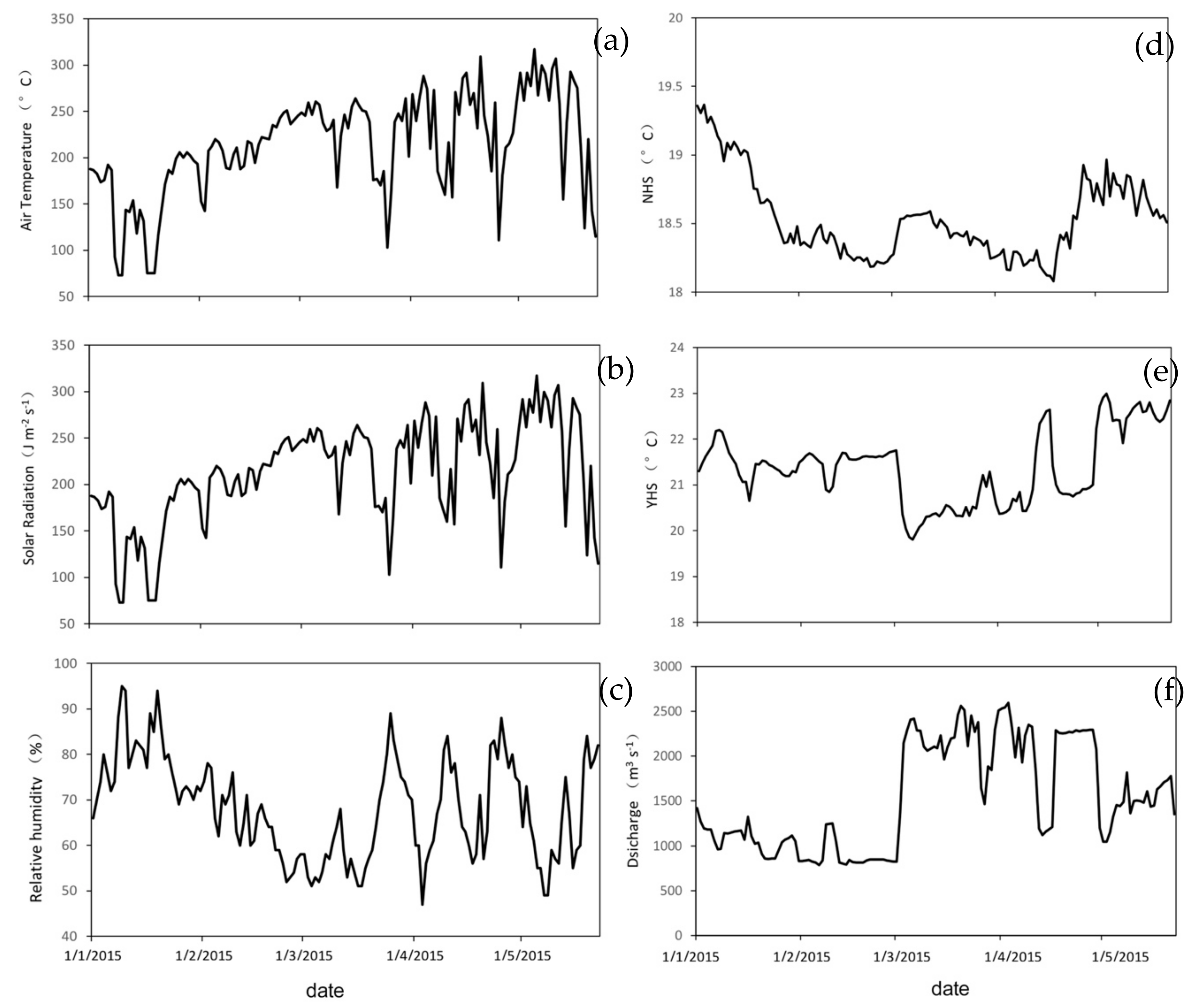
Daily meteorological data (1 January 2015 to 20 May 2015) measured at the Jinghong National Meteorological Station: (a) air temperature, (b) solar radiation, and (c) relative humidity. Water temperature data is measured at the NHS and YHS station: (d) water temperature at NHS, (e) water temperature at YHS, and (f) discharge at YHS.
Figure 5.
Daily meteorological data (1 January 2015 to 20 May 2015) measured at the Jinghong National Meteorological Station: (a) air temperature, (b) solar radiation, and (c) relative humidity. Water temperature data is measured at the NHS and YHS station: (d) water temperature at NHS, (e) water temperature at YHS, and (f) discharge at YHS.

Figure 6.
Flowchart of the Jinghong Reservoir model set-up.
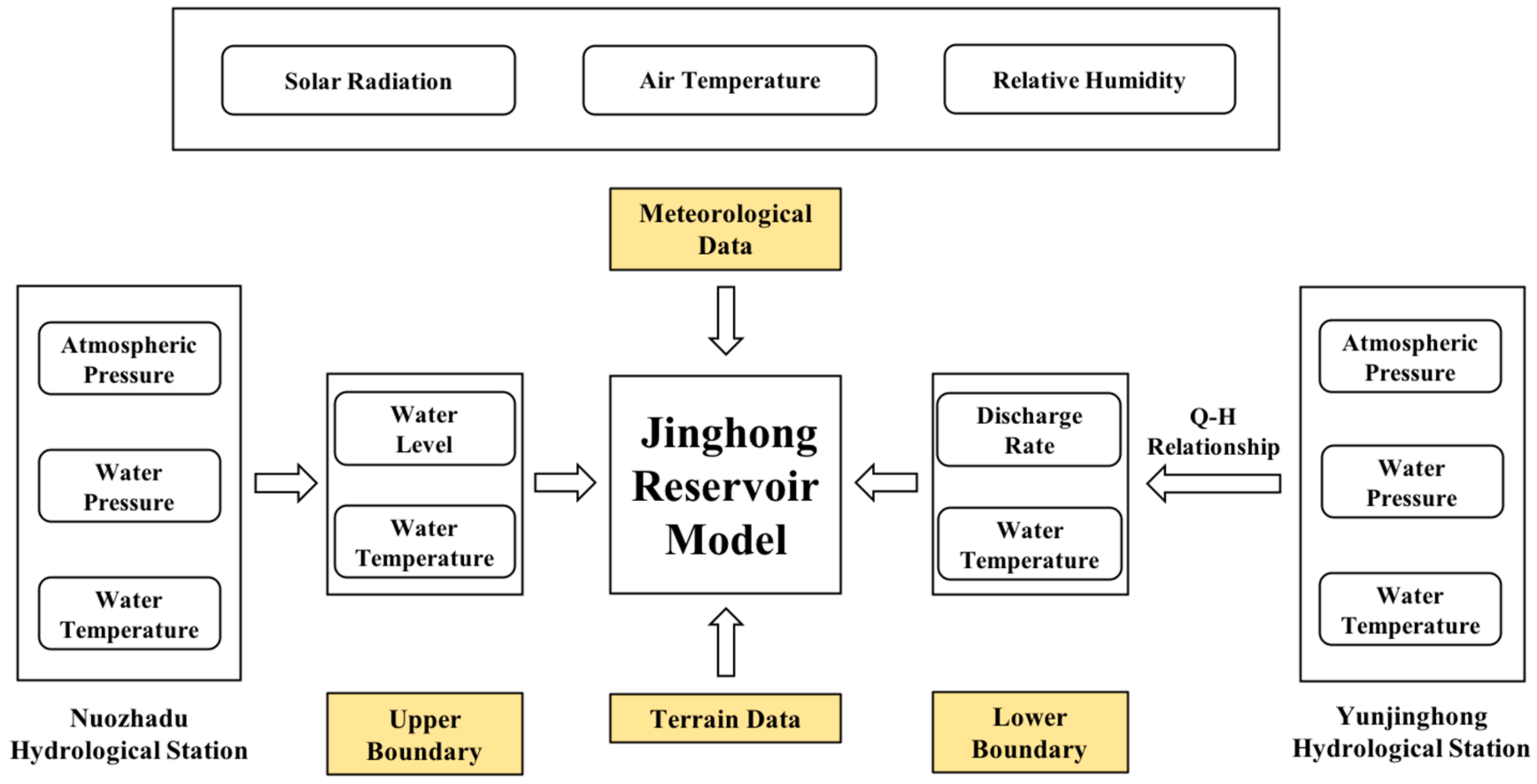
Figure 7.
Comparison between simulated and measured water levels at Simao Harbor. Simulated water levels are plotted on an hourly average.
Figure 7.
Comparison between simulated and measured water levels at Simao Harbor. Simulated water levels are plotted on an hourly average.
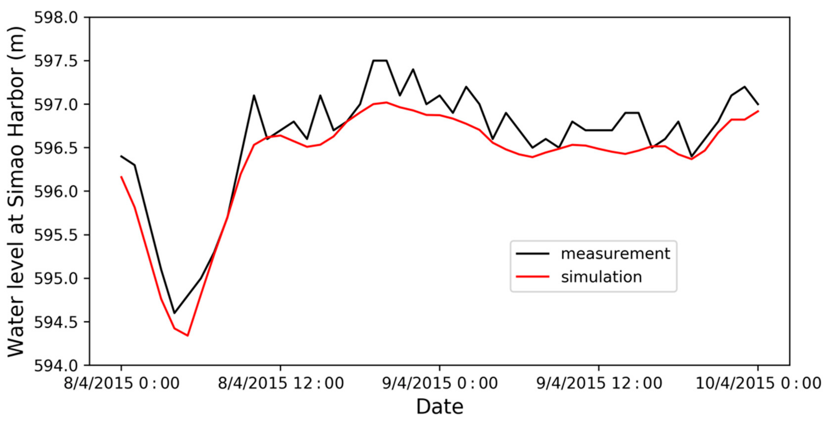
Figure 8.
Outlet water temperature difference between the simulation results (CTL) and measurements at YHS.
Figure 8.
Outlet water temperature difference between the simulation results (CTL) and measurements at YHS.
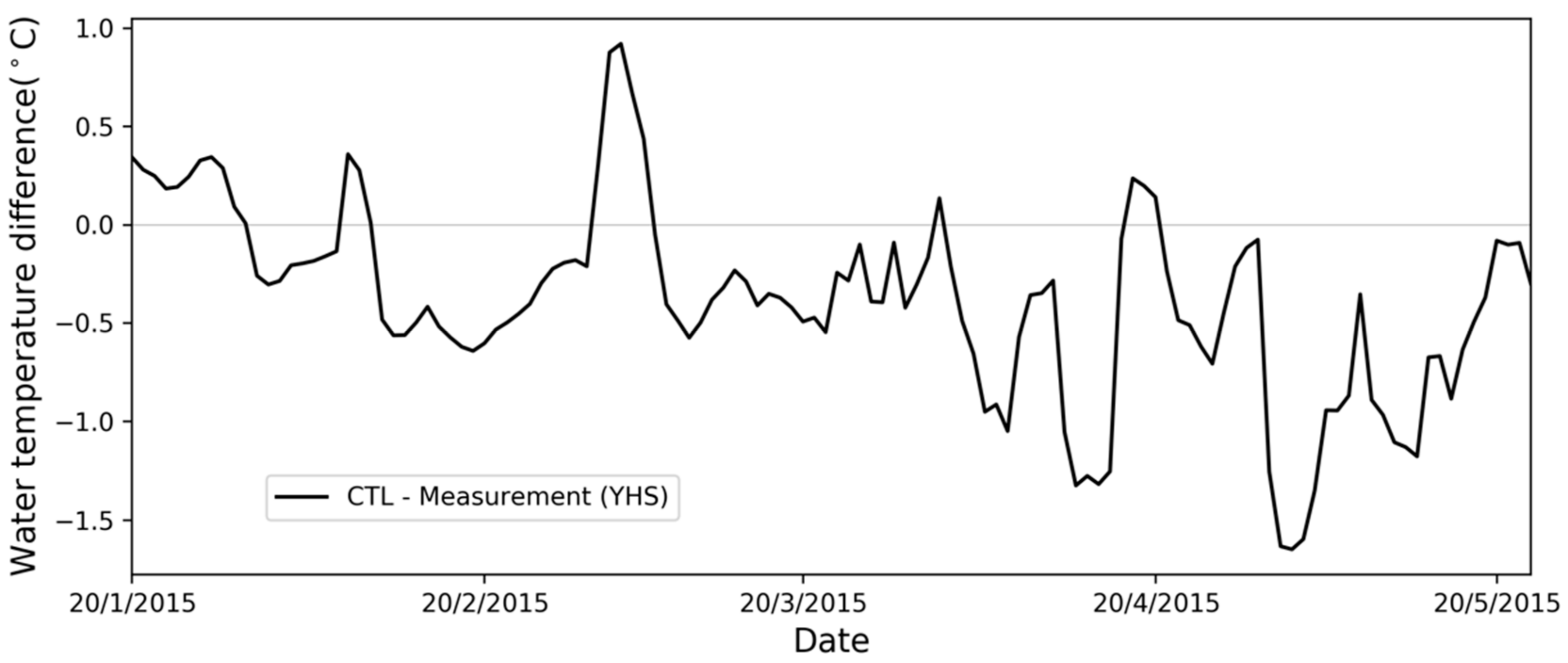
Figure 9.
Simulated water temperature profile along the reservoir on (a) 15th March, (b) 15th April, and (c) 15th May of 2015.
Figure 9.
Simulated water temperature profile along the reservoir on (a) 15th March, (b) 15th April, and (c) 15th May of 2015.


Figure 10.
Simulated water temperature by CTL, S2, and S3 at the YHS. The measured water temperature at the NHS and air temperature at the Nuozhadu Dam are shown for reference. The vertical blue line indicates the boundary of the period when air temperature was significantly lower than water temperature at the YHS.

Figure 11.
Respective contributions of solar radiation and atmosphere-water heat exchange to the water temperature at the YHS on a weekly scale. Negative contribution values mean that the factor had a decreasing effect on water temperature. Contribution values are computed based on the extent of water temperature changes, taking the water temperature difference between CTL and S3 as 100%.

Figure 12.
(a) Tracer concentration variations at the YHS corresponding to various outflow rates (F2, F4, F6, and F8 are demonstrated in the figure); and (b) the exponential relationship between residence time and outflow rate of the Jinghong Reservoir.
Figure 12.
(a) Tracer concentration variations at the YHS corresponding to various outflow rates (F2, F4, F6, and F8 are demonstrated in the figure); and (b) the exponential relationship between residence time and outflow rate of the Jinghong Reservoir.
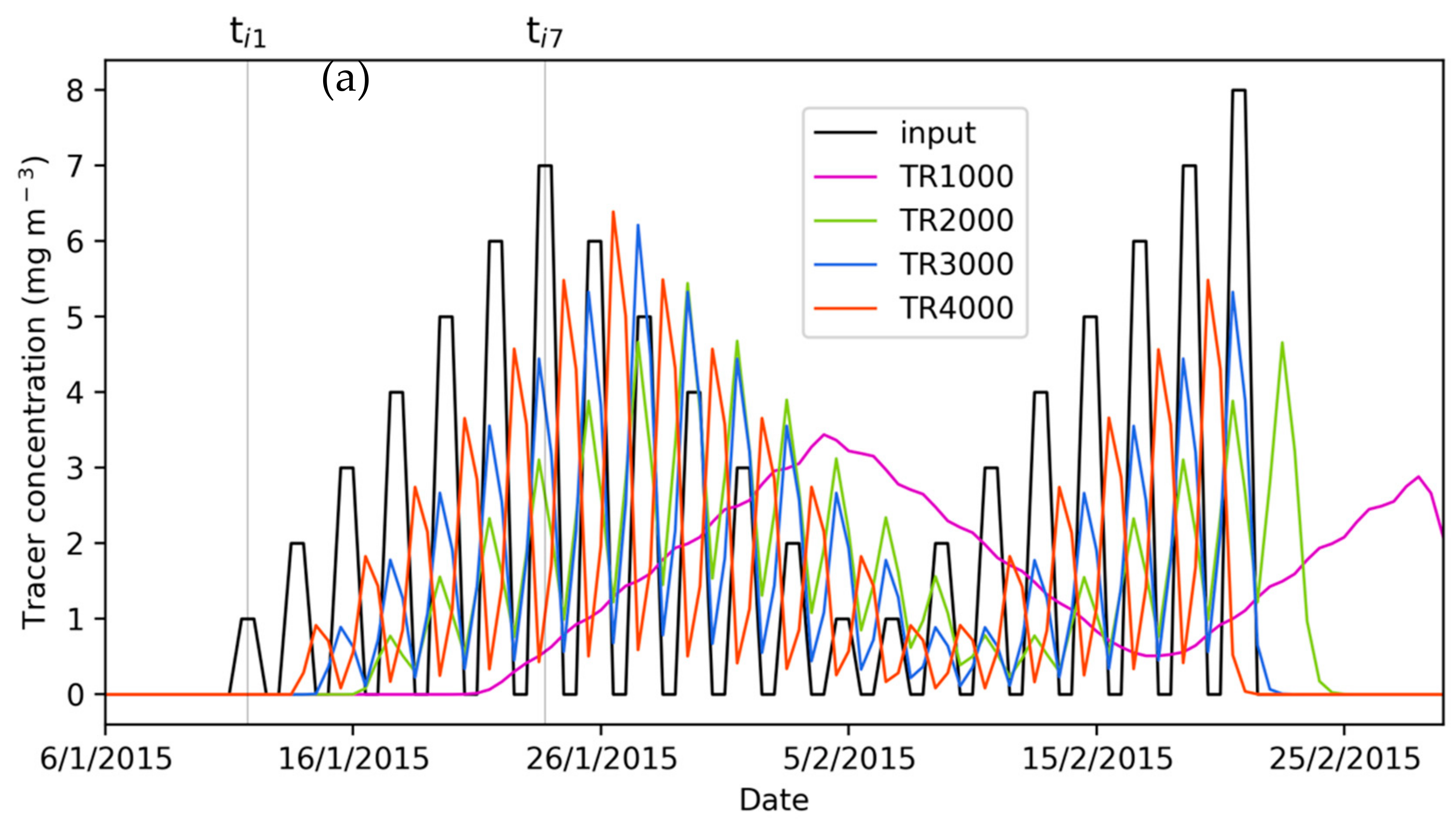
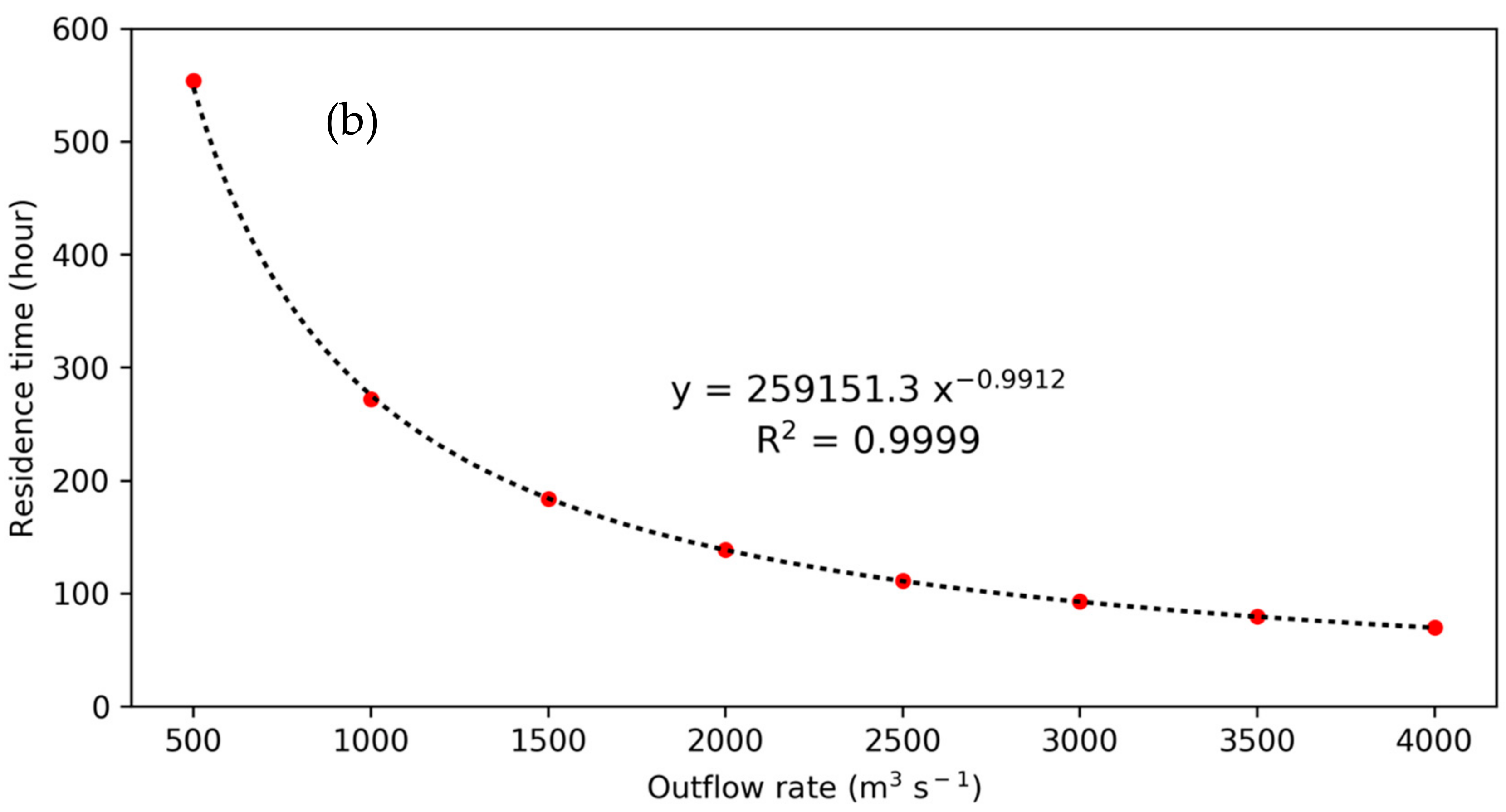
Figure 13.
(a) Relationship between outflow rate and water temperature difference (outflow minus inflow); and (b) relationship between residence time and water temperature difference at the YHS.
Figure 13.
(a) Relationship between outflow rate and water temperature difference (outflow minus inflow); and (b) relationship between residence time and water temperature difference at the YHS.

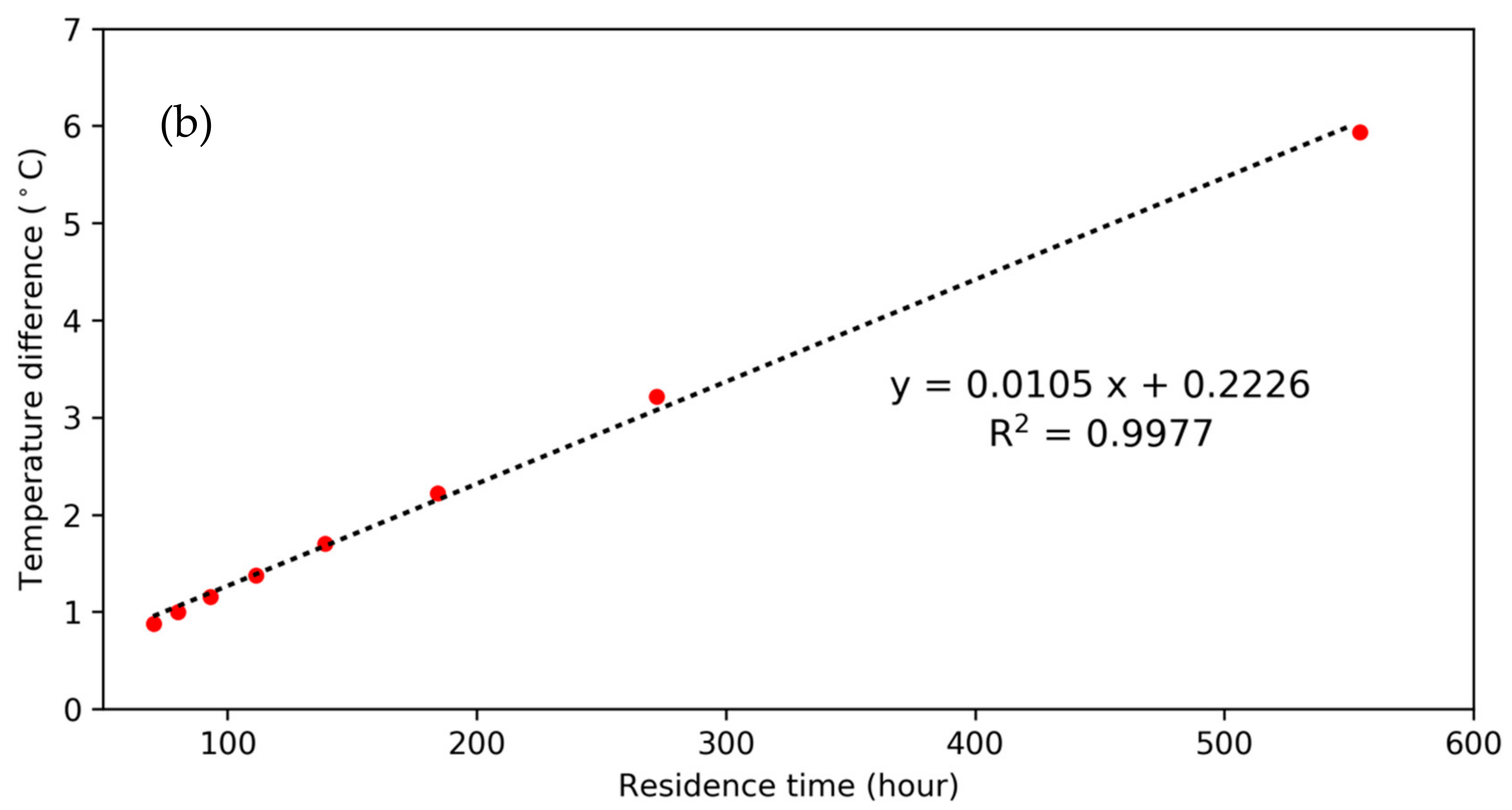
Figure 14.
Simulated water temperature during the study period by CTL and S1 at the YHS, and measured water temperature at the NHS and historical water temperature (1997–2004) at the YHS.
Figure 14.
Simulated water temperature during the study period by CTL and S1 at the YHS, and measured water temperature at the NHS and historical water temperature (1997–2004) at the YHS.

Table 1.
Parameters studied for the calibration of the Jinghong Reservoir model and their chosen value.
Table 1.
Parameters studied for the calibration of the Jinghong Reservoir model and their chosen value.
| Parameter | Studied Range | Chosen Value |
|---|---|---|
| Chezy’s coefficient | 10–100 m½ s−1 | 65 m½ s−1 |
| Background horizontal eddy viscosity | 1 × 10⁻⁶–1 m2 s−1 | 5 × 10⁻⁴ m2 s−1 |
| Background horizontal eddy diffusivity | 1 × 10⁻⁶–1 m2 s−1 | 1 × 10⁻⁴ m2 s−1 |
| Background vertical eddy viscosity | 1 × 10⁻¹⁰–1 m2 s−1 | 1 × 10⁻⁶ m2 s−1 |
| Background vertical eddy diffusivity | 1 × 10⁻¹⁰–1 m2 s−1 | 1 × 10⁻⁶ m2 s−1 |
Table 2.
An overview of numerical experiments.
| Experiments | The Jinghong Reservoir | Solar Radiation | Atmosphere-Water Heat Exchange | Outflow Rate (m3 s−1) | Tracer |
|---|---|---|---|---|---|
| CTL | ON | ON | ON | Real | OFF |
| S1 | OFF | ON | ON | Real | OFF |
| S2 | ON | OFF | ON | Real | OFF |
| S3 | ON | OFF | OFF | Real | OFF |
| F1 | ON | ON | ON | 500 | ON |
| F2 | ON | ON | ON | 1000 | ON |
| F3 | ON | ON | ON | 1500 | ON |
| F4 | ON | ON | ON | 2000 | ON |
| F5 | ON | ON | ON | 2500 | ON |
| F6 | ON | ON | ON | 3000 | ON |
| F7 | ON | ON | ON | 3500 | ON |
| F8 | ON | ON | ON | 4000 | ON |
Table 3.
The α index of three major reservoirs along the middle and lower reaches of the Lancang River and their thermal structure type according to the index.
Table 3.
The α index of three major reservoirs along the middle and lower reaches of the Lancang River and their thermal structure type according to the index.
| Reservoir Name | Average Annual Inflow (billion m3) | Total Capacity (billion m3) | α Index | Type |
|---|---|---|---|---|
| Xiaowan | 38.2 | 15.1 | 2.5 | Stably stratified |
| Nuozhadu | 55.5 | 23.7 | 2.3 | Stably stratified |
| Jinghong | 58.0 | 1.1 | 25.4 | Mixed |
© 2018 by the authors. Licensee MDPI, Basel, Switzerland. This article is an open access article distributed under the terms and conditions of the Creative Commons Attribution (CC BY) license (http://creativecommons.org/licenses/by/4.0/).
Share and Cite
MDPI and ACS Style
Jiang, B.; Wang, F.; Ni, G. Heating Impact of a Tropical Reservoir on Downstream Water Temperature: A Case Study of the Jinghong Dam on the Lancang River. Water 2018, 10, 951. https://doi.org/10.3390/w10070951
AMA Style
Jiang B, Wang F, Ni G. Heating Impact of a Tropical Reservoir on Downstream Water Temperature: A Case Study of the Jinghong Dam on the Lancang River. Water. 2018; 10(7):951. https://doi.org/10.3390/w10070951
Chicago/Turabian StyleJiang, Bo, Fushan Wang, and Guangheng Ni. 2018. "Heating Impact of a Tropical Reservoir on Downstream Water Temperature: A Case Study of the Jinghong Dam on the Lancang River" Water 10, no. 7: 951. https://doi.org/10.3390/w10070951
Note that from the first issue of 2016, this journal uses article numbers instead of page numbers. See further details here.