Article

Spatial Pattern Oriented Multicriteria Sensitivity Analysis of a Distributed Hydrologic Model

1
Geological Survey of Denmark and Greenland, Øster Voldgade 10, 1350 Copenhagen, Denmark
2
Department of Civil Engineering, Istanbul Technical University, Maslak, 34469 Istanbul, Turkey
3
Department of Environmental Engineering, Technical University of Denmark, 2800 Kgs. Lyngby, Denmark
*
Authors to whom correspondence should be addressed.
Water 2018, 10(9), 1188; https://doi.org/10.3390/w10091188
Submission received: 10 August 2018 / Revised: 29 August 2018 / Accepted: 1 September 2018 / Published: 4 September 2018
(This article belongs to the Special Issue Hydrologic Modelling for Water Resources and River Basin Management)

Abstract

:
Hydrologic models are conventionally constrained and evaluated using point measurements of streamflow, which represent an aggregated catchment measure. As a consequence of this single objective focus, model parametrization and model parameter sensitivity typically do not reflect other aspects of catchment behavior. Specifically for distributed models, the spatial pattern aspect is often overlooked. Our paper examines the utility of multiple performance measures in a spatial sensitivity analysis framework to determine the key parameters governing the spatial variability of predicted actual evapotranspiration (AET). The Latin hypercube one-at-a-time (LHS-OAT) sampling strategy with multiple initial parameter sets was applied using the mesoscale hydrologic model (mHM) and a total of 17 model parameters were identified as sensitive. The results indicate different parameter sensitivities for different performance measures focusing on temporal hydrograph dynamics and spatial variability of actual evapotranspiration. While spatial patterns were found to be sensitive to vegetation parameters, streamflow dynamics were sensitive to pedo-transfer function (PTF) parameters. Above all, our results show that behavioral model definitions based only on streamflow metrics in the generalized likelihood uncertainty estimation (GLUE) type methods require reformulation by incorporating spatial patterns into the definition of threshold values to reveal robust hydrologic behavior in the analysis.

1. Introduction

Computer models are indispensable to perform costly experiments in an office environment, e.g., distributed modelling of water fluxes across the hydrosphere. Physically based distributed hydrologic models have become increasingly complex due to the large number of incorporated parameters to represent a variety of spatially distributed processes. These models are typically calibrated against stream gauge observations, i.e., a lumped variable of all hydrological processes at catchment scale. This can cause equifinality problems [1] and poor performance of the simulated spatial pattern of the model since optimizing the water balance and streamflow dynamics are the only concern [2,3]. To solve this issue, the community needs models with flexible spatial parametrization and calibration frameworks that incorporate spatially distributed observations, e.g., remote sensing estimates of evapotranspiration (ET).
The basic idea behind any sensitivity analysis (SA) method is to relate the response of the model output to variations in the parameter values [4]. The SA methods can, therefore, enhance our control on spatiotemporal model behavior [5]. There are local (LSA) and global sensitivity analysis (GSA) methods that evaluate distinct and joint effects between different model parameters, respectively [6,7,8].
While LSA methods evaluate point sensitivity in parameter space [9], the GSA covers the entire parameter space and parameter interactions too [10,11]. This is because GSA perturbs all parameters simultaneously to assess the inter-relations [12]. The most well-known GSA methods are Sobol’s method [13] and the Fourier amplitude sensitivity test (FAST) [14]. The main effects (e.g., first-order sensitivity) and elementary effects, originally described by Morris [15], can be evaluated using both methods. The Morris method has been widely applied in hydrologic modelling. Herman et al. [16] were able to classify parameters of a spatially distributed watershed model as sensitive and not sensitive based on the Morris method with 300 times fewer model evaluations than Sobol’s approach. The GSA methods are usually thought to be more appropriate to use in hydrologic applications than LSA methods since hydrological processes are nonlinear and the interactions between the parameters have a substantial effect on the results. However, the computational cost is crucial in applying the GSA methods in distributed hydrologic modelling [17,18]. The LSA methods gives fast results by assessing only one parameter at a time without interactions between parameters [19]. The local derivatives are, however, based on a certain initial set in the parameter space.
The foremost objective of our study is to assess the major driving parameters for the spatial patterns of actual evapotranspiration (AET) simulated by a catchment model. Furthermore, we address how the selected initial set of parameters can affect the LSA results and how many initial sets are required for a robust sensitivity analysis. We evaluate parameter sensitivities using an LSA method with random and behavioral initial parameter sets (each containing 100 initial parameter sets). We focus on both spatial patterns of AET over the basin and temporal hydrograph dynamics using multiple performance metrics to evaluate different aspects of the simulated maps and the hydrograph. Streamflow performance of a model has typically been the main concern in conventional model calibrations, whereas improving the simulated spatial pattern during calibration has rarely been targeted [20,21,22,23,24,25,26]. A unique feature of our study is evaluating the model’s sensitivity based on a set of 10 spatial metrics that, unlike traditional cell-to-cell metrics, provide true pattern information. We include an innovative metric which utilizes empirical orthogonal function analysis [23] as well as the fractional skill score [27], among others, to evaluate the simulated spatial patterns. The added value of each metric is assessed based on a redundancy test. This is done to identify the most robust metric(s) with unique information content to apply in a subsequent spatial calibration study.
Höllering et al. [28] used hydrologic fingerprint-based sensitivity analysis using temporally independent and temporal dynamics of only streamflow data. They could identify two major driving parameters for evapotranspiration and soil moisture dynamics in different mesoscale catchments in Germany and reveal their relation to different streamflow characteristics. Westerhoff [29] used remotely sensed ET data as an interpolator between point data and used a simplified sensitivity analysis only focusing on interpolation between ground-based estimates based on simple (linear) relationships. In our study, we took it up another notch by using the spatial pattern, including sensitivity analyses, using multiple methods, for improved hydrological model calibration. We tested a large range of methods and spatial metrics. Also, we applied the mesoscale hydrologic model (mHM) [30] which can simulate distributed variables using pedo-transfer functions (PTF) and related parameters. Additionally, a recently introduced dynamic ET scaling function (DSF) was used to increase the physical control on simulated spatial patterns of AET [2]. Ultimately, the identified important parameters for simulating both stream discharge and spatial patterns of AET were used in a very recent model calibration study [2]. The novelty of the current study lies in using sensitivity maps showing the difference between the initial run and perturbation of a parameter and various spatial metrics to complement conventional SA with spatial pattern evaluation.

2. Materials

The Skjern River has a basin area of ~2500 km2 covered by mostly sandy soils (Figure 1) and dominated by agriculture (71%) and forest (15%) [21]. The maximum altitude in the basin is 130 m and annually averaged precipitation is around 1000 mm [31]. The monthly mean temperatures vary between 2 and 17 degrees Celsius whereas the annual mean streamflow is around 475 mm [32].

2.1. Satellite-Based Data

We used different products from the Moderate Resolution Imaging Spectroradiometer (MODIS) (Table 1) to generate leaf area index (LAI) and AET maps. The data were retrieved from NASA Land Processes Distributed Active Archive Center (LP-DAAC).

2.1.1. Leaf Area Index (LAI)

The Nadir BRDF Adjusted Reflectance (NBAR) from the MCD43B4 product was used to calculate the normalized vegetation index (NDVI) [34]. Subsequently, the dataset was smoothed using a temporal filter available in the TIMESAT code [35,36]. Due to the low data availability of the MODIS LAI product at the latitudes of the study site during some periods of the year, we derived a new empirical LAI equation based on the NDVI, (Equation (1)).
Since in situ measurements of LAI are scarce and typically limited to specific crops, the reference LAI data used for the empirical equation was obtained from the LAI input tables for the Danish National Water Resources model [37,38]. The most common land use type in Denmark is cropland, ~80% of the total area. Boegh et al. [39] derived LAI using remote sensing data with an exponential function. In our case, we used a similar approach in the following equation:
L A I = 0.0633 5.524     N D V I
Using different equations for different land cover types is possible. However, imposing a land cover map on the remote sensing inputs can predispose the maps to show a spatial pattern controlled by land cover. To minimize this effect, we decided to apply a single equation to derive the LAI, i.e., established based on the most abundant land cover type (agricultural) in the study area. The derived 8-day LAI product was later linearly interpolated to obtain daily LAI values for each pixel, which we found suitable for the study area, because temporal variability is limited at this time scale.

2.1.2. Actual Evapotranspiration (TSEB)

The Two Source Energy Balance (TSEB) model developed by Norman et al. [40] based on Priestly-Taylor approximation [41] was incorporated in this study to estimate AET based on MODIS data. The model inputs were solar zenith angle (SZA) and land surface temperature (LST) as well as height of canopy and albedo levels, all derived from MODIS based observations. Other climate variables of incoming radiation and air temperature were retrieved from European Centre for Medium-Range Weather Forecasts reanalysis data interim version (ERA-interim) [42]. One-at-a-time sensitivity analysis [43] of the TSEB model revealed that LST is the most sensitive parameter for AET (results not shown here). The TSEB model output was evaluated against field observations of eddy fluxes over three different land cover types before deriving the final maps of AET. The main purpose of including the remote-sensing-based AET estimations was to evaluate the spatial pattern performance of the model data during the growing season. All data were averaged across all years for calibration and validation periods to six monthly averaged spatial maps from April to September. This was because uncertainty is inevitable in the individual daily estimates of AET, whereas the monthly maps show the general monthly patterns, which are more robust. We referred to this AET data as reference data to evaluate mHM-based simulations of AET. We chose reference instead of observation, as the data were not purely observed but were an energy balance model output using satellite observations.

2.2. Hydrologic Model

The mesoscale hydrologic model (mHM) has been developed as a distributed model delivering different outputs and fluxes at different model scales [30]. The direct runoff, slow and fast interflow, and base flow are calculated for every grid cell. Finally, the runoff is routed through the basin domain using the Muskingum flood routing method. The model applies pedo-transfer functions to regionalize soil parameters and is easily set up for different platforms, e.g., Mac, Linux, and Windows. The model contains 53 parameters for calibration. The nonlinear dynamic ETref scaling function introduced in an earlier study [2] has flexibility to change the spatial pattern of AET during the sensitivity analysis as a function of vegetation as compared to the uniform or aspect-driven PET correction factor originally implemented in mHM (Table 2). The study by Samaniego et al. [30] is the key reference describing model formulation and parameter description.
Meteorological input at different spatial scales can be handled internally by the model. This underlines the flexibility of mHM which operates at three spatial scales: morphologic data scale (L0), model scale (L1), and meteorological data (L2). The model scale, i.e., L1, can have any value between L0 and L2. In our case, the Skjern model ran at a daily time scale at 1 × 1 km resolution, whereas the soil inputs had a 250 × 250 m resolution. The meteorological datasets, i.e., P, ETref, and Tavg, were gridded observational data from the Danish Meteorological Institute resampled from a native resolution of 10 and 20 km, respectively [2]. Readers are referred to Table 1 in Demirel et al. [2] for the complete list of model inputs and data sources.

3. Methods

In this study, we applied the Latin hypercube sampling strategy [44] combined with a local sensitivity analysis approach [19]. Latin hypercube sampling, firstly named after McKay et al. [44], is an efficient multidimensional sampling similar to Monte Carlo sampling (MCS) but requiring much fewer runs to avoid the clumpy size of uniform random sampling [45]. It splits the range of each variable into different intervals of equal probability, where one value is randomly selected from each interval [46]. This improves the stability of MCS while preserving the tractability of random sampling.
We tested 10 sophisticated performance measures (hereinafter called objective functions) to identify most important parameters. Three of these metrics, i.e., Nash–Sutcliffe Efficiency (NSE, Nash and Sutcliffe [47]), Kling–Gupta Efficiency (KGE, Gupta et al., [48]), and percent bias (PB), focus on simulated streamflow, whereas the remaining objective functions focus on the spatial distribution of AET (Table 3). Although PB is included in KGE equation, the PB that reflects errors in the water balance was evaluated separately to consider volume error in addition to the streamflow timing.

3.1. Objective Functions Focusing on Spatial Patterns

The objective functions focusing on streamflow, i.e., NSE, KGE, and PB, are all well known and therefore not presented in detail. In the following, we focus on introducing the spatial objective functions. Seven objective functions were used to evaluate the pattern similarity between the reference AET from TSEB and the simulated AET from mHM. Five of the seven spatial-pattern-oriented metrics are calculated based on the spatial overlap of categorical maps [54]. In this study, we used three classes to transform the continuous patterns of AET into categorical maps: (1) below the 15th percentile, (2) above the 85th percentile, and (3) the remaining grids between highest 15% and lowest 15% values. The empirical orthogonal functions analysis does not require categorical maps and therefore does not need to be transformed. The fractional skill score is based on categorical maps but uses more bins in the classification than the three mentioned above. The applied spatial metrics are all bias insensitive, which we consider favorable to conduct a meaningful pattern comparison. The overall water balance error is well represented by streamflow observations and therefore represented in the respective objective functions. Moreover, AET is simulated in mm/day, whereas the remote sensing reference is given in W/m2. The two units are closely related but vary in range; therefore, applying bias insensitive metrics is inevitable.

3.1.1. Goodman and Kruskal’s Lambda

Goodman and Kruskal’s lambda ( λ ) is a similarity metric for contingency tables. It has an optimal value of one indicating perfect match and lowest value of zero indicating no overlap [55]. λ is calculated as
λ = i = 1 m m a x j ( c i j ) + i = 1 m m a x j ( c i j ) m a x j ( c + j ) m a x i ( c i + ) 2 N m a x j ( c + j ) m a x i ( c i + )
where N is the total number of grids; m is the number of classes in the observed maps to be compared; cij is the grid numbers for the class i in first map (A) and to class j in the second map (B); c i + is the grid numbers contained in category i in map A; c + j is the grid numbers contained in category j in map B; m a x i ( c i + ) is the grid numbers in the modal class of map A, i.e., the class with largest number of grids; and m a x j ( c i j ) is the number of classes in map B with a given class of map A.

3.1.2. Theil’s Uncertainty Coefficient

Theil’s Uncertainty (U) is a measure of percent reduction in error. It is also known as average mutual information [55]. It yields the same value when the reference map is A or B, i.e., symmetric; therefore, a reference does not need to be defined. Unlike λ which accounts for modal class, Theil’s U considers the whole distribution of the data. It is based on entropy, joint entropy, and average mutual information [50,54]. The information content (entropy) of map A is calculated as
H ( A ) = i = 1 m c i + N log ( c i + N )
The same notation as λ is used for Theil’s U equation below. Similarly for map B:
H ( B ) = j = 1 m c + j N log ( c + j N ) .
The joint entropy is then calculated as
H ( A , B ) = i = 1 m j = 1 n c i j N log ( c i j N ) .
The shared information by maps A and B is estimated by average mutual information I(A;B) based on the entropy of two maps minus the joint entropy:
I ( A ; B ) = H ( A ) + H ( B ) H ( A , B ) .
The uncertainty coefficient is then calculated as
U = 2     I ( A ; B ) H ( A ) + H ( B ) .

3.1.3. Cramér’s V

Cramér’s V is a metric based on Pearson’s X 2 statistic calculated from the contingency table of maps A and B [51]. Recently, Speich et al. [54] used this metric to assess the similarity of different bivariate maps for Switzerland. In their case, the variable pairs snowmelt and runoff as well as precipitation and PET were selected to describe the water balance in Swiss catchments. The χ 2 statistics can be calculated by
χ 2 = i = 1 m j = 1 n ( c i j c i + c + j / N ) 2 c i + c + j / N
using the same notation of c i j , c i + , and c + j as for the metrics above. In addition, m and n show the number of grids in maps A and B, respectively. χ 2 always yields non-negative values. Zero values only appear in the case when c i j = c i + c + j / N .The zero value hence indicates no similarity between the map pairs. There have been different modifications of χ 2 [55], but the simplest and most widely used form was proposed by Cramér [51]. V is a transformation of X 2 , as shown below:
V = χ 2 N     ( min ( m , n ) 1 )
In an earlier study, Rees [55] used Cramér’s V together with two other categorical association metrics (U and λ ) to assess the similarity of two thematic maps from Landsat images. All three metrics investigated in that study appeared to work well, as they produced significantly high values for the maps that were reasonably similar and low values for those maps that obviously differed. Rees [55] recommended using Cramér’s V for three reasons: (1) this metric is relatively simple to calculate; (2) it is symmetric, giving the same value when the reference map is A or B; and (3) it performs slightly better than U and λ in discriminating between two different maps or approving two similar maps.

3.1.4. Mapcurves

Mapcurves (MC) is a measure of goodness-of-fit (GOF), indicating the degree of match between two categorical maps [54]. It has an optimal value of one, whereas the lowest value is zero. For each pair of classes (i, j) between the two maps A and B, the algorithm calculates GOF using the following equation:
G O F i j = c i j c i +   c i j c + j
In the following equations, the equations are presented for class A (i.e., index i), as the category A represents observed maps and B indicates simulated maps (i.e., index j). Thus, the calculation for class B is analogous. The GOF values are added up for each group of the observed map (A):
G A , i = j = 1 n G i j
where n is the grid numbers in the map (A). Note that the size of the maps should match each other for this comparison. The GOF values are organized in ascending order to estimate the vector G A . The values 0 and 1 are included in the series of G A to integrate the function later. The length of G A is hence m + 2. For each GOF value i G A , the MC is calculated as a segment of classes that have a GOF more than or equal to i:
f A ( i ) = k = 1 m [ G A , k i ] m ; i   ϵ   G A
The MC value is then calculated by integrating f(x) between zero and one. A trapezoid rule is applied as follows to calculate the area under the curve. It has a best value of one.
M C A = i = 1 n ( G A , i + 1 G A , i )    f A ( x + 1 ) + ( G A , i + 1 G A , i )    ( f A ( x + 1 ) f A ( x ) ) 2

3.1.5. Empirical Orthogonal Functions

The empirical orthogonal functions (EOF) analysis is a frequently applied tool to study the spatiotemporal variability of environmental and meteorological variables [56,57]. The most important feature of the EOF analysis is that it decomposes the variability of a spatiotemporal dataset into two crucial components, i.e., time-invariant orthogonal spatial patterns and a set of loadings that are time variant [2]. Perry et al. [56] gave a brief description of the mathematical background of the EOF analysis. The EOF-based similarity score (SEOF) at time x is formulated as
S E O F x = i = 1 n w i | ( l o a d i s i m ( x ) l o a d i o b s ( x ) ) |
where n is the number of EOFs and wi represents the covariation contribution of the ith EOF. In our study, we focused on the overall AET pattern performance and thus we averaged SEOF from the individual months of the growing season into a single overall skill score.

3.1.6. Fractions Skill Score

Roberts and Lean [27] introduced the fractions skill score (FSS) to the atmospheric science community to establish a quantitative measure of how the skill of precipitation products varies for different spatial scales. Fractions relate to occurrences of values exceeding a certain threshold at a given window size (scale) and are compared between model and observation at individual grids. Most commonly, the thresholds represent percentiles which have the purpose of eliminating any impact of a potential bias. Hence, FSS assesses the spatial performance of a model as a function of threshold and scale and has been implemented by Gilleland et al. [58], Wolff et al. [59], and others to spatially validate precipitation forecasts. In summary, the following steps are performed during the FSS methodology: (1) truncate the observed A and simulated B spatial patterns into binary patterns for each threshold of interest, (2) compute fractions A(n) and B(n) within a given spatial scale n based on the number of grids that exceed the threshold and lie within the window of size n by n, and (3) estimate the mean-squared-error (MSE) and standardize it with a worst-case MSE that returns zero spatial agreement between A and B (MSEref). The MSE is based on all grids (Nxy) that define the catchment area with dimension Nx and Ny. For a certain threshold, the FSS at scale n is given by
F S S ( n ) = 1 M S E ( n ) M S E ( n ) r e f
where
M S E ( n ) = 1 N x y i = 1 N x j = 1 N y [ A ( n ) i j B ( n ) i j ] 2
and
M S E ( n ) r e f = 1 N x y [ i = 1 N x j = 1 N y A ( n ) i j 2 + i = 1 N x j = 1 N y B ( n ) i j 2 ]
FSS ranges from zero to one, where one indicates a perfect agreement between observed and simulated patterns and zero reflects the worst possible performance. To our knowledge, Koch et al. [60] were the first to transfer FSS from the atmospheric to the hydrological community and applied it on spatial patterns of land-surface variables simulated by a hydrological catchment model. The flexibility of FSS, in terms of scale and threshold, is very desirable in hydrological modelling applications where uncertainties in model forcing and parameters as well as scale differences between model and observation hinder a meaningful validation at native scales. In this study, FSS was implemented in an automated manner. In order to reduce the computational time, an overall FSS score was computed based on an average of six selected percentiles with individual thresholds. We decided to tolerate placement errors of extreme percentiles (1% and 99% that focus on the bottom and top 1% of AET, respectively) more than moderate percentiles (20% and 80%) by assessing the first at a larger scale (25 km) than the latter (5 km). In addition, the 5th and 95th percentiles, which represent the top and bottom 5% of AET grids, were assessed at a 15-km scale. The average of these six percentiles was used as the overall FSS score.

3.2. Latin Hypercube Sampling One-Factor-at-a-Time Sensitivity Analysis

We used Latin hypercube (LH) sampling in combination with a local sensitivity analysis method. This is an integration of a global sampling method with a local SA method changing one factor at a time (OAT). In other words, one perturbation at a time depends on the local derivatives based on a certain initial point in the parameter space [19]. A similar design based on random perturbation at a time following trajectories was firstly proposed by Morris [15]. SA based on Monte Carlo simulation is robust but requires a larger number of simulations. Alternatively, the LHS is based on a stratified sampling method that divides the parameter values into N strata with probability of occurrence having a value of 1/N. This feature leads to a more robust sensitivity analysis with a given number of initial values [
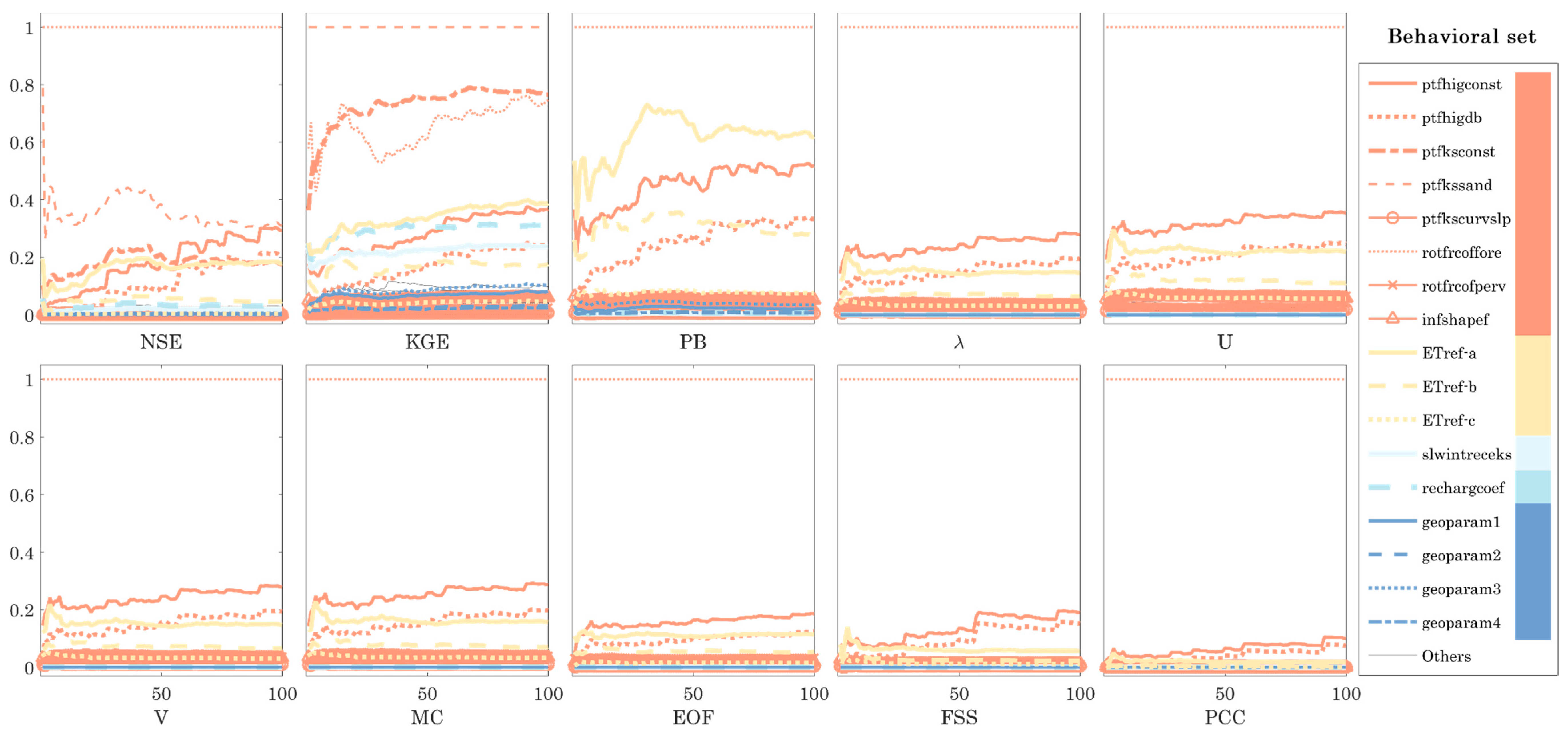
19]. Here, we tested whether behavioral initial parameter sets resulted in different parameter identification compared to random initial parameter sets. In addition, we used 100 different initial sets to assess if/when the accumulated relative sensitivities became stable. We could then evaluate how many initial samples were required to get robust results using LHS-OAT.

4. Results

4.1. Exploration of Spatial Metrics Characteristics

The spatial performance metrics were examined to gain more insight into their reliability and to understand whether any of them provided redundant information. This is an important step before including them in the sensitivity analysis and model calibration because the ability to discriminate between a good and a poor spatial pattern performance is an essential characteristic of a metric. We compared 12 synthetic land surface temperature (LST) maps of a sub-basin of Skjern (~1000 km2), i.e., all perturbed differently, with a reference LST map using the spatial metrics applied in this study. The details about the applied perturbation strategies can be found in Table 1 of Koch et al. [23]. In that study, Koch et al. [23] conducted an online-based survey with the aim of using the well-trained human perception to rank the 12 synthetic LST maps in terms of their similarity to the reference map. The obtained results were subsequently used to benchmark a set of spatial performance metrics. The same procedure was incorporated in this study to get a better understanding of the metrics selected for this study. We included the survey results in our study and assessed the coefficient of determination R2 between the human perception and the spatial metrics. This helped to differentiate between metrics that contained redundant information and those with unique information content. Figure 2 shows two distinct examples, i.e., one noisy perturbation and one slightly similar map to the reference map, to better explain the results presented in Table 4, which summarizes the spatial scores for the 12 maps sorted based on the survey similarity index (last column).
Map 9 is ranked as the second least similar map as compared to the reference map. Map 10 that is perturbed with an overall bias of +2 is ranked as a perfect agreement by all metrics. This confirms that all of our spatial metrics are bias insensitive. In addition, map 1 is identified as the most similar map to the reference map by the human perception and all other metrics.
Following the R2 values in Table 5, 72.2% of the variance in the human perception is explained by the EOF analysis. The Pearson correlation coefficient (PCC), V, and FSS metrics also performed well in discriminating spatial maps with respect to the human perception as benchmark. However, the U metric explained the lowest variance (40.9%), which indicates that it should not be included in the model calibration because we trust the well-trained human perception as a reference. Moreover, the spatial metrics, i.e., λ, U, V, and MC, are highly correlated (italic fonts in Table 5). All are based on transforming the data into a three category system, which results in redundancy between the four given metrics. This shows that not all of them are required for model calibration. However, we will still evaluate the sensitivity results based on all given spatial metrics in the following sections.

4.2. Latin Hypercube Sampling One-Factor-at-a-Time Sensitivity Analysis

In this study, we applied LHS-OAT sensitivity analysis with 47 parameters using both random and behavioral sets of initial parameter values. Initially, we selected 100 random initial parameter sets using the lower and upper limits of the parameters. Subsequently, we generated 10,000 random initial samples to select 100 behavioral sets among these. For that, we started running each of the 10,000 random sets one at a time and evaluated the simulated discharge. We continued the model runs until we reached 100 behavioral sets that all resulted in NSE above 0.5. This is because we were interested in investigating only the plausible region of the parameter space, as we knew the calibration would never end up outside this region in either way. We also ensured that the selected 100 behavioral sets were uniformly distributed to the different probability bins since we tested only the first ~2400 random initial parameter sets to have 100 behavioral sets.
In total, we executed mHM about ~11,800 times in forward mode using the parameter estimation tool PEST [43]. This is because we ran the model ~4700 times (47 parameters × 100 LHS-OAT) for random and ~4700 times for behavioral initial sets and performed an additional ~2400 runs for the selection of a behavioral set as described above. Figure 3 shows the average accumulated relative parameter sensitivities over the 100 behavioral (NSE > 0.5) initial parameter sets and one-at-a-time parameter perturbations. The average accumulated relative parameter sensitivities became stable, i.e., unchanging parameter ranking, after ~20 initial parameter sets were used in LHS-OAT. Relative sensitivities were normalized values by the highest sensitive parameter. Therefore, the most sensitive parameter resulted in one. It should be noted that we only show the results of behavioral initial sets as they are similar to those from the random initial sets. Here, the colored lines show the most important parameters. Other parameters are presented in gray color only. One of the soil moisture related parameter (rotfrcoffore) is always the most sensitive parameter for all objective functions except for KGE, where one parameter of the PTF, i.e., related to sandy soils, is the most sensitive one as compared to the other 47 parameters of mHM. The rankings of important parameters are converged and similar for all spatial objective functions, while different parameters are highlighted using streamflow-related objective functions. The five most sensitive parameters based on spatial objective functions are soil-moisture-related, PTF, and ET-related parameters. Further, ETref-a parameter seems to be the second most important parameter affecting streamflow dynamics of the Skjern River model (see PB at Figure 3 and Figure 4), whereas another PTF parameter is ranked as the second most important parameter affecting KGE (Table A1).
Figure 4 shows sensitivities calculated from modeled AET using the average of 100 maps, where each reflects the impact of a perturbation per parameter based on the 100 behavioral (NSE > 0.5) parameter sets as initial points. Each of these 100 perturbation maps (sensitivity maps) were calculated as the absolute difference between the initial run and the perturbation that was further normalized by the initial run, i.e., NMAD (%) = abs(perturbation-initial)/initial. We then used the average of 100 runs as a final sensitivity map. The maps in Figure 4 are informative in several ways. First, they show that some of the parameters have a uniform (light green map) or no effect (dark blue map) on the spatial pattern distribution, whereas other parameters have a high control on spatial variability (e.g., rotfrcofperv, ptfkssand, and ETref-a). Second, we can recognize different patterns on the maps such as land cover patterns (see Figure 1) from root fraction maps (especially the one for pervious areas), LAI patterns from ETref-c map, and soil patterns from pedo-transfer function maps (e.g., ptfksconst). The geoparam 2, 3, and 4 parameters are also identified as sensitive influencing streamflow dynamics (see KGE at Figure 3). However, their maps are not shown in Figure 4 as they are similar to the map for geoparam 1 (uniform effect). Further, the map for the ptflowdb parameter is completely dark blue, showing that it has no effect on the simulated spatial pattern of AET.

4.3. Random Parameter Sets Based on the 17 Sensitive Parameters Evaluated against NSE and FSS

Figure 5 illustrates the simulated spatial AET performance as a function of streamflow model performance based on 1700 randomly generated parameter sets only constrained by the parameter bounds and evaluated against observed streamflow and spatial patterns of AET. Only the results of 329 parameter sets from 1700 total random sample resulting a minimum NSE of 0.0 are shown in these two plots, i.e., the left plot shows NSE vs. FSS and right plot shows NSE vs. EOF. In the generalized likelihood uncertainty estimation (GLUE)-based uncertainty analysis framework, numerous random parameter sets are sampled and, from those, only the parameter sets that deliver a performance level that is above a predefined minimum threshold are retained and classified as behavioral models [61]. As a rule of thumb, 10% of the random parameter sets should be behavioral. Demirel et al. [62] generated 120,000 parameter sets for a conceptual hydrologic model and around 10,000 (~9%) parameter sets were selected using a threshold, i.e., NSE above 0.4. This performance measure has been widely used in rainfall-runoff model optimizations and subsequent GLUE studies. Additional performance measures can constrain the solution space and decrease the number of behavioral models. Wambura et al. [26] showed that while 100 out of 1000 random parameter sets satisfied the hydrograph performance evaluation based on NSE above 0.65 threshold, only 80 behavioral models could be identified with two performance measures, i.e., NSE and index of volumetric fit. Similarly, in this study, the behavioral models from a discharge criterion (NSE above 0.5) exhibited very different spatial AET performances, varying from ~0.1 to ~0.8 for both FSS and EOF (Figure 5). Using a simple 10% (~35 parameter sets) cutoff provided a subjective threshold value of above 0.5 for FSS and below 0.15 for EOF. Together with NSE above 0.5, these two thresholds enabled the identification of a more robust selection of behavioral model regions, shown with a green box shown in Figure 5. It should be noted that the number of runs that satisfy both spatial metrics and NSE is 20, which is considerably less than using only one spatial metric. Both spatial metrics clearly indicate that the set of behavioral models is narrowed considerably by adding spatial patterns to the definition of combined behavioral threshold. Therefore, inclusion of MODIS AET to the sensitivity analysis only improves the quality and robustness of the behavioral model selection. Moreover, the results from Figure 5 illustrate the potential of spatial pattern evaluation to discriminate between behavioral parameter sets from more than a pure NSE perspective and how it can minimize equifinality issues.

5. Discussion

In this study, we identified important parameters for streamflow dynamics and spatial patterns of AET by incorporating different spatial and temporal performance metrics in an LHS-OAT sensitivity analysis combined with spatial sensitivity maps. We first analyzed the suitability of spatial performance metrics for sensitivity analysis. The results suggest that a good combination of performance metrics that are complementary should be included in a sensitivity analysis. Most importantly, the metrics should be able to separate similar and dissimilar spatial patterns. We concluded this by benchmarking a set of performance metrics against human perception, which is a reliable and well-trained reference for comparing spatial patterns. Furthermore, redundant metrics need to be identified and excluded from the analysis.
Another important point is that the modeler has to select or design a model parametrization scheme that allows the simulated spatial patterns to change while minimizing the number of model parameters. Otherwise, the efforts towards a spatial model calibration will be inadequate. Here, the mHM model was selected due to its flexibility through the pedo-transfer functions.
Once the appropriate spatial performance metrics and model are selected, model evaluation against relevant spatial observations can be conducted. We are aware that the use of another model could lead to different sensitivities and thus different conclusions. Such modelling schemes can be easily incorporated with any parameter sensitivity analysis. In our study, the identified parameters that were sensitive to either streamflow or spatial patterns were used in a subsequent calibration framework. With this study, we ensured that we selected the best combination of objective functions for model calibration and simultaneously reduced the computational costs of model calibration by reducing the number of model parameters.

Utility of the Multicriteria Spatial Sensitivity Analysis

To compensate the weakness of one-at-a-time perturbation, we incorporated different random and behavioral initial sets in our study. This made the combined approach simple and robust when used with appropriate multiple metrics. It should be noted that LHS-OAT has been validated in different study areas [5,19]. Although the parameter interactions are not evaluated explicitly, the identified parameters seem to be the most important and relevant parameters for calibration. This might stem from the fact that parameters in mHM are not highly interacting with each other, as already shown in Cuntz et al. [18]. The resultant maps in Figure 4 are instrumental in deciding which parameter has a spatial effect on the results. The saturation after 20 initial sets (Figure 3) corresponds to 940 model simulations (20 × 47), including 47 mHM parameters evaluated in LHS-OAT. These are much fewer numbers of runs as compared to first and second order sensitivity analysis based on Sobol’s approach, which requires a minimum of 104–105 model simulations [63,64]. The gain in computational costs is mostly due to the fact that we are not mainly interested in quantitative sensitivity indexes but rather the importance ranking of the model parameters. Here, we showed that the LHS-OAT method can reduce the computational burden of the GSA methods such as Sobol’s.
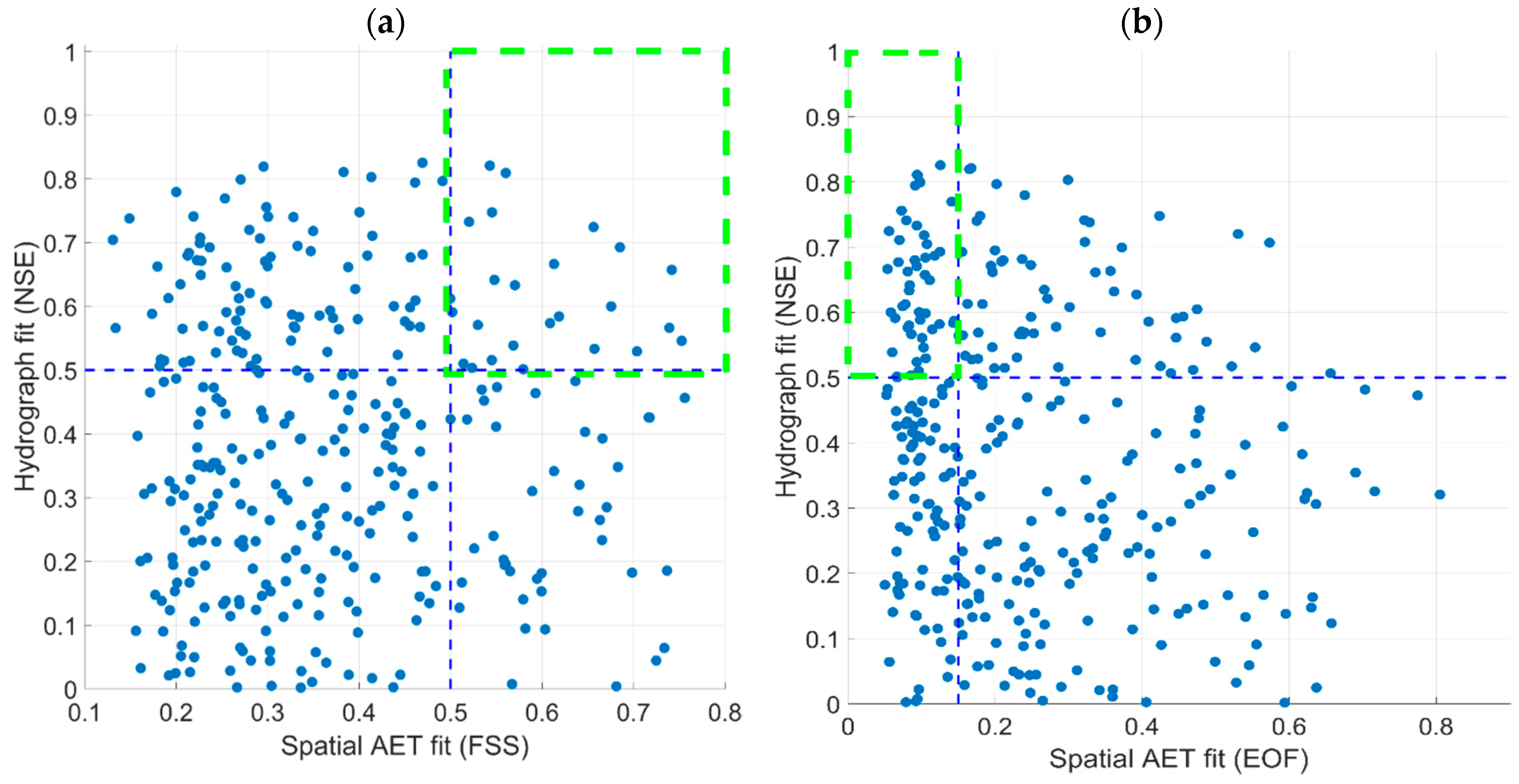
In this study, we could exemplify the impact of selecting thresholds of 0.5 for FSS and 0.15 for EOF on the selection of behavioral models, although it is recognized that these thresholds are case specific and rather arbitrary. While the use of NSE for streamflow evaluation over the past five decades has built familiarity with this metric and generated a consensus on thresholds for behavioral models regarding streamflow, these thresholds are also arbitrary and differ slightly from one study to another. It is anticipated that once the spatial metrics are used more often in hydrologic modelling practices, expertise in identifying suitable performance metrics and threshold values for satisfying spatial performances will grow. Particularly for the GLUE type uncertainty analysis methods and other model calibration frameworks, a new spatiotemporal perspective for behavioral model definition is indispensable. The framework described in this study does not aim at replacing discharge as a hydrologic model evaluation target, however, it strongly encourages that spatial data on, e.g., AET, are used in conjunction with point discharge data when evaluating distributed models. By gradually making spatial pattern evaluation an integral part of standard distributed model evaluation and performance reporting, it is anticipated that the hydrologic community will build a similar familiarity with spatial performance metrics as has been built with discharge metrics.

6. Conclusions

The effect of hydrologic model parameters on the spatial distribution of AET has been evaluated with LHS-OAT method and maps. This was done to identify the most sensitive parameters to both streamflow dynamics and monthly spatial patterns of AET. To increase the model’s ability to change simulated spatial patterns during calibration, we introduced a new dynamic scaling function using actual vegetation information to update reference evapotranspiration at the model scale. Moreover, the uncertainties arising from random and behavioral Latin hypercube sampling were addressed. The following conclusions can be drawn from our results:
  • Based on the detailed analysis of spatial metrics, the EOF, FSS, and Cramér’s V are found to be relevant (nonredundant) pairs for spatial comparison of categorical maps. Further, the PCC metric can provide an easy understanding of map association, although it can be very sensitive to extreme values.
  • Based on the results from sensitivity analysis, vegetation and soil parametrization mainly control the spatial pattern of the actual evapotranspiration in the mHM model for this study area.
  • Besides, the interception, recharge, and geological parameters are also important for changing streamflow dynamics. Their effect on spatial actual evapotranspiration pattern is substantial but uniform over the basin. For interception, the lacking effect on the spatial pattern of AET is due to the exclusion of rainy days in the spatial pattern evaluation.
  • More than half of the 47 parameters included in this study have either little or no effect on simulated spatial patterns, i.e., noninformative parameters, in the Skjern Basin with the chosen setup. In total, only 17 of 47 mHM parameters were selected for a subsequent spatial calibration study.
  • The sensitivity maps are consistent with parameter types, as they reflect land cover, LAI, and soil maps of the Skjern Basin.
  • Combining NSE with a spatial metric strengthens the physical meaningfulness and robustness of selecting behavioral models.
Our results are in line with the study by Cornelissen et al. [24] showing that spatial parameterization directly affects the monthly AET patterns simulated by the hydrologic model. Further, Berezowski et al. [5] used a similar sort of Latin hypercube one-factor-at-a-time algorithm for sensitivity analysis of model parameters affecting simulated snow distribution patterns over the Biebrza River catchment in Poland. However, to our knowledge, this is the first study incorporating sensitivity maps with a wide range of spatial performance metrics. The LHS-OAT method is easy to apply and informative when used with bias-insensitive spatial metrics. The framework is transferrable to other catchments in the world. Even other metrics can be added to the spatial metric group if not redundant with the current ones.

Author Contributions

M.C.D. and S.S. designed the sensitivity analysis framework, conducted model runs and prepared some of the figures. J.K. conducted experiments on human perception, provided some of the metric codes (EOF and FSS), and prepared some of the figures. G.M. prepared remote sensing data, mean monthly reference raster images and post processing python codes.

Funding

This research was funded by Villum Fonden VKR023443 and Turkish Scientific and Technical Research Council 118C020.

Acknowledgments

The authors acknowledge the financial support for the SPACE project by the Villum Foundation (http://villumfonden.dk/) through their Young Investigator Program (grant VKR023443). The first author is supported by Turkish Scientific and Technical Research Council. We also thank Manuel Antonetti and Massimiliano Zappa from Swiss Federal Institute WSL for providing the R codes to estimate three spatial indices, i.e., Goodman and Kruskal’s Lambda, Theil’s U and Cramér’s V. We also acknowledge Emiel E. van Loon from University of Amsterdam who provides the R code to calculate Mapcurves index at http://staff.fnwi.uva.nl/e.e.vanloon/code/mapcurves.zip. The code for the EOF analysis and FSS is freely available from the SEEM GitHub repository (https://github.com/JulKoch/SEEM). The repository also contains the maps used in the spatial similarity survey and the associated similarity rating based on the human perception. The TSEB code is retrieved from https://github.com/hectornieto/pyTSEB. All MODIS data was retrieved from the online Data Pool, courtesy of the NASA Land Processes Distributed Active Archive Center (LP DAAC), USGS/Earth Resources Observation and Science (EROS) Center, Sioux Falls, South Dakota, https://lpdaac.usgs.gov/data_access/data_pool.

Conflicts of Interest

The authors declare no conflict of interest.

Appendix A

Table A1. Comparison of sensitive parameters using different methods.
IDParameterDescriptionNormalized Sensitivity
LHS-OAT RandomLHS-OAT Behavioral
KGEFSSKGEFSS
1ptfhigconstConstant in pedo-transfer function (ptf) for soils with sand content higher than 66.5%0.3940.2070.3670.19
2ptfhigdbCoefficient for bulk density in pedo-transfer function for soils with sand content higher than 66.5%0.2610.170.2430.151
3ptfksconstConstant in pedo-transfer function for hydraulic conductivity of soils with sand content higher than 66.5%0.3660.0030.7650.005
4ptfkssandCoefficient for sand content in pedo-transfer function for hydraulic conductivity 0.4690.00510.006
5ptfkscurvslpExponent in pedo-transfer function for hydraulic conductivity to adjust slope of curve0.0050.0020.0070.004
6rotfrcofforeRoot fraction for forested areas110.7461
7rotfrcofpervRoot fraction for pervious areas0.030.0080.0240.01
8infshapefInfiltration (inf) shape factor0.0510.0080.060.011
9ETref-aIntercept0.3830.0520.3880.056
10ETref-bBase coefficient0.1650.0210.1760.022
11ETref-cExponent coefficient0.0460.0080.0470.011
12slwintreceksSlow (slw) interception0.11300.2360
13rechargcoefRecharge coefficient (coef)0.1400.3090
14geoparam1Parameter for first geological formation0.1300.0810
15geoparam2Parameter for second geological formation0.04500.0320
16geoparam3Parameter for third geological formation0.17500.1050
17geoparam4Parameter for fourth geological formation0.03800.0250

References

  1. Beven, K.; Freer, J. Equifinality, data assimilation, and uncertainty estimation in mechanistic modelling of complex environmental systems using the GLUE methodology. J. Hydrol. 2001, 249, 11–29. [Google Scholar] [CrossRef]
  2. Demirel, M.C.; Mai, J.; Mendiguren, G.; Koch, J.; Samaniego, L.; Stisen, S. Combining satellite data and appropriate objective functions for improved spatial pattern performance of a distributed hydrologic model. Hydrol. Earth Syst. Sci. 2018, 22, 1299–1315. [Google Scholar] [CrossRef] [Green Version]
  3. Koch, J.; Demirel, M.C.; Stisen, S. The SPAtial EFficiency metric (SPAEF): Multiple-component evaluation of spatial patterns for optimization of hydrological models. Geosci. Model Dev. 2018, 11, 1873–1886. [Google Scholar] [CrossRef]
  4. Shin, M.-J.; Guillaume, J.H.A.; Croke, B.F.W.; Jakeman, A.J. Addressing ten questions about conceptual rainfall–runoff models with global sensitivity analyses in R. J. Hydrol. 2013, 503, 135–152. [Google Scholar] [CrossRef]
  5. Berezowski, T.; Nossent, J.; Chormański, J.; Batelaan, O. Spatial sensitivity analysis of snow cover data in a distributed rainfall-runoff model. Hydrol. Earth Syst. Sci. 2015, 19, 1887–1904. [Google Scholar] [CrossRef] [Green Version]
  6. Saltelli, A.; Tarantola, S.; Chan, K.P.-S. A Quantitative Model-Independent Method for Global Sensitivity Analysis of Model Output. Technometrics 1999, 41, 39–56. [Google Scholar] [CrossRef]
  7. Bahremand, A. HESS Opinions: Advocating process modeling and de-emphasizing parameter estimation. Hydrol. Earth Syst. Sci. 2016, 20, 1433–1445. [Google Scholar] [CrossRef] [Green Version]
  8. Zhuo, L.; Han, D. Could operational hydrological models be made compatible with satellite soil moisture observations? Hydrol. Process. 2016, 30, 1637–1648. [Google Scholar] [CrossRef]
  9. Rakovec, O.; Hill, M.C.; Clark, M.P.; Weerts, A.H.; Teuling, A.J.; Uijlenhoet, R. Distributed Evaluation of Local Sensitivity Analysis (DELSA), with application to hydrologic models. Water Resour. Res. 2014, 50, 409–426. [Google Scholar] [CrossRef] [Green Version]
  10. Massmann, C.; Holzmann, H. Analysis of the behavior of a rainfall–runoff model using three global sensitivity analysis methods evaluated at different temporal scales. J. Hydrol. 2012, 475, 97–110. [Google Scholar] [CrossRef]
  11. Bennett, K.E.; Urrego Blanco, J.R.; Jonko, A.; Bohn, T.J.; Atchley, A.L.; Urban, N.M.; Middleton, R.S. Global Sensitivity of Simulated Water Balance Indicators Under Future Climate Change in the Colorado Basin. Water Resour. Res. 2018, 54, 132–149. [Google Scholar] [CrossRef]
  12. Lilburne, L.; Tarantola, S. Sensitivity analysis of spatial models. Int. J. Geogr. Inf. Sci. 2009, 23, 151–168. [Google Scholar] [CrossRef] [Green Version]
  13. Sobol, I. Global sensitivity indices for nonlinear mathematical models and their Monte Carlo estimates. Math. Comput. Simul. 2001, 55, 271–280. [Google Scholar] [CrossRef]
  14. Cukier, R.I. Study of the sensitivity of coupled reaction systems to uncertainties in rate coefficients. I Theory. J. Chem. Phys. 1973, 59, 3873. [Google Scholar] [CrossRef]
  15. Morris, M.D. Factorial Sampling Plans for Preliminary Computational Experiments. Technometrics 1991, 33, 161–174. [Google Scholar] [CrossRef] [Green Version]
  16. Herman, J.D.; Kollat, J.B.; Reed, P.M.; Wagener, T. Technical Note: Method of Morris effectively reduces the computational demands of global sensitivity analysis for distributed watershed models. Hydrol. Earth Syst. Sci. 2013, 17, 2893–2903. [Google Scholar] [CrossRef]
  17. Razavi, S.; Gupta, H. What Do We Mean by Sensitivity Analysis? The Need for Comprehensive Characterization of ‘Global’ Sensitivity in Earth and Environmental Systems Models. Water Resour. Res. 2015, 51, 3070–3092. [Google Scholar] [CrossRef]
  18. Cuntz, M.; Mai, J.; Zink, M.; Thober, S.; Kumar, R.; Schäfer, D.; Schrön, M.; Craven, J.; Rakovec, O.; Spieler, D.; et al. Computationally inexpensive identification of noninformative model parameters by sequential screening. Water Resour. Res. 2015, 51, 6417–6441. [Google Scholar] [CrossRef] [Green Version]
  19. Van Griensven, A.; Meixner, T.; Grunwald, S.; Bishop, T.; Diluzio, M.; Srinivasan, R. A global sensitivity analysis tool for the parameters of multi-variable catchment models. J. Hydrol. 2006, 324, 10–23. [Google Scholar] [CrossRef]
  20. Stisen, S.; Jensen, K.H.; Sandholt, I.; Grimes, D.I.F.F. A remote sensing driven distributed hydrological model of the Senegal River basin. J. Hydrol. 2008, 354, 131–148. [Google Scholar] [CrossRef]
  21. Larsen, M.A.D.; Refsgaard, J.C.; Jensen, K.H.; Butts, M.B.; Stisen, S.; Mollerup, M. Calibration of a distributed hydrology and land surface model using energy flux measurements. Agric. For. Meteorol. 2016, 217, 74–88. [Google Scholar] [CrossRef] [Green Version]
  22. Melsen, L.; Teuling, A.; Torfs, P.; Zappa, M.; Mizukami, N.; Clark, M.; Uijlenhoet, R. Representation of spatial and temporal variability in large-domain hydrological models: Case study for a mesoscale pre-Alpine basin. Hydrol. Earth Syst. Sci. 2016, 20, 2207–2226. [Google Scholar] [CrossRef]
  23. Koch, J.; Jensen, K.H.; Stisen, S. Toward a true spatial model evaluation in distributed hydrological modeling: Kappa statistics, Fuzzy theory, and EOF-analysis benchmarked by the human perception and evaluated against a modeling case study. Water Resour. Res. 2015, 51, 1225–1246. [Google Scholar] [CrossRef] [Green Version]
  24. Cornelissen, T.; Diekkrüger, B.; Bogena, H. Using High-Resolution Data to Test Parameter Sensitivity of the Distributed Hydrological Model HydroGeoSphere. Water 2016, 8, 202. [Google Scholar] [CrossRef]
  25. Cai, G.; Vanderborght, J.; Langensiepen, M.; Schnepf, A.; Hüging, H.; Vereecken, H. Root growth, water uptake, and sap flow of winter wheat in response to different soil water conditions. Hydrol. Earth Syst. Sci. 2018, 22, 2449–2470. [Google Scholar] [CrossRef] [Green Version]
  26. Wambura, F.J.; Dietrich, O.; Lischeid, G. Improving a distributed hydrological model using evapotranspiration-related boundary conditions as additional constraints in a data-scarce river basin. Hydrol. Process. 2018, 32, 759–775. [Google Scholar] [CrossRef]
  27. Roberts, N.M.; Lean, H.W. Scale-Selective Verification of Rainfall Accumulations from High-Resolution Forecasts of Convective Events. Mon. Weather Rev. 2008, 136, 78–97. [Google Scholar] [CrossRef]
  28. Höllering, S.; Wienhöfer, J.; Ihringer, J.; Samaniego, L.; Zehe, E. Regional analysis of parameter sensitivity for simulation of streamflow and hydrological fingerprints. Hydrol. Earth Syst. Sci. 2018, 22, 203–220. [Google Scholar] [CrossRef] [Green Version]
  29. Westerhoff, R.S. Using uncertainty of Penman and Penman-Monteith methods in combined satellite and ground-based evapotranspiration estimates. Remote Sens. Environ. 2015, 169, 102–112. [Google Scholar] [CrossRef]
  30. Samaniego, L.; Kumar, R.; Attinger, S. Multiscale parameter regionalization of a grid-based hydrologic model at the mesoscale. Water Resour. Res. 2010, 46. [Google Scholar] [CrossRef] [Green Version]
  31. Stisen, S.; Sonnenborg, T.O.; Højberg, A.L.; Troldborg, L.; Refsgaard, J.C. Evaluation of Climate Input Biases and Water Balance Issues Using a Coupled Surface–Subsurface Model. Vadose Zone J. 2011, 10, 37–53. [Google Scholar] [CrossRef]
  32. Jensen, K.H.; Illangasekare, T.H. HOBE: A Hydrological Observatory. Vadose Zone J. 2011, 10, 1–7. [Google Scholar] [CrossRef]
  33. Mendiguren, G.; Koch, J.; Stisen, S. Spatial pattern evaluation of a calibrated national hydrological model—A remote-sensing-based diagnostic approach. Hydrol. Earth Syst. Sci. 2017, 21, 5987–6005. [Google Scholar] [CrossRef]
  34. Tucker, C.J. Red and photographic infrared linear combinations for monitoring vegetation. Remote Sens. Environ. 1979, 8, 127–150. [Google Scholar] [CrossRef] [Green Version]
  35. Jonsson, P.; Eklundh, L. Seasonality extraction by function fitting to time-series of satellite sensor data. IEEE Trans. Geosci. Remote Sens. 2002, 40, 1824–1832. [Google Scholar] [CrossRef]
  36. Jönsson, P.; Eklundh, L. TIMESAT—A program for analyzing time-series of satellite sensor data. Comput. Geosci. 2004, 30, 833–845. [Google Scholar] [CrossRef]
  37. Stisen, S.; Højberg, A.L.; Troldborg, L.; Refsgaard, J.C.; Christensen, B.S.B.; Olsen, M.; Henriksen, H.J. On the importance of appropriate precipitation gauge catch correction for hydrological modelling at mid to high latitudes. Hydrol. Earth Syst. Sci. 2012, 16, 4157–4176. [Google Scholar] [CrossRef] [Green Version]
  38. Refsgaard, J.C.; Stisen, S.; Højberg, A.L.; Olsen, M.; Henriksen, H.J.; Børgesen, C.D.; Vejen, F.; Kern-Hansen, C.; Blicher-Mathiesen, G. Danmarks Og Grønlands Geologiske Undersøgelse Rapport 2011/77; Geological Survey of Danmark and Greenland (GEUS): Copenhagen, Denmark, 2011. [Google Scholar]
  39. Boegh, E.; Thorsen, M.; Butts, M.; Hansen, S.; Christiansen, J.; Abrahamsen, P.; Hasager, C.; Jensen, N.; van der Keur, P.; Refsgaard, J.; et al. Incorporating remote sensing data in physically based distributed agro-hydrological modelling. J. Hydrol. 2004, 287, 279–299. [Google Scholar] [CrossRef]
  40. Norman, J.M.; Kustas, W.P.; Humes, K.S. Source approach for estimating soil and vegetation energy fluxes in observations of directional radiometric surface temperature. Agric. For. Meteorol. 1995, 77, 263–293. [Google Scholar] [CrossRef]
  41. Priestley, C.H.B.; Taylor, R.J. On the Assessment of Surface Heat Flux and Evaporation Using Large-Scale Parameters. Mon. Weather Rev. 1972, 100, 81–92. [Google Scholar] [CrossRef] [Green Version]
  42. Dee, D.P.; Uppala, S.M.; Simmons, A.J.; Berrisford, P.; Poli, P.; Kobayashi, S.; Andrae, U.; Balmaseda, M.A.; Balsamo, G.; Bauer, P.; et al. The ERA-Interim reanalysis: Configuration and performance of the data assimilation system. Q. J. R. Meteorol. Soc. 2011, 137, 553–597. [Google Scholar] [CrossRef]
  43. Doherty, J. PEST: Model Independent Parameter Estimation. Fifth Edition of User Manual; Watermark Numerical Computing: Brisbane, Australia, 2005. [Google Scholar]
  44. McKay, M.D.; Beckman, R.J.; Conover, W.J. A Comparison of Three Methods for Selecting Values of Input Variables in the Analysis of Output from a Computer Code. Technometrics 1979, 21, 239–245. [Google Scholar]
  45. Du, S.; Wang, L. Aircraft Design Optimization with Uncertainty Based on Fuzzy Clustering Analysis. J. Aerosp. Eng. 2016, 29, 04015032. [Google Scholar] [CrossRef]
  46. Chu, L. Reliability Based Optimization with Metaheuristic Algorithms and Latin Hypercube Sampling Based Surrogate Models. Appl. Comput. Math. 2015, 4. [Google Scholar] [CrossRef]
  47. Nash, J.E.; Sutcliffe, J.V. River flow forecasting through conceptual models part I—A discussion of principles. J. Hydrol. 1970, 10, 282–290. [Google Scholar] [CrossRef]
  48. Gupta, H.V.; Kling, H.; Yilmaz, K.K.; Martinez, G.F. Decomposition of the mean squared error and NSE performance criteria: Implications for improving hydrological modelling. J. Hydrol. 2009, 377, 80–91. [Google Scholar] [CrossRef] [Green Version]
  49. Goodman, L.A.; Kruskal, W.H. Measures of Association for Cross Classifications*. J. Am. Stat. Assoc. 1954, 49, 732–764. [Google Scholar] [CrossRef]
  50. Finn, J.T. Use of the average mutual information index in evaluating classification error and consistency. Int. J. Geogr. Inf. Syst. 1993, 7, 349–366. [Google Scholar] [CrossRef]
  51. Cramér, H. Mathematical Methods of Statistics; Princeton University Press: Princeton, NJ, USA, 1946; ISBN 0-691-08004-6. [Google Scholar]
  52. Hargrove, W.W.; Hoffman, F.M.; Hessburg, P.F. Mapcurves: A quantitative method for comparing categorical maps. J. Geogr. Syst. 2006, 8, 187–208. [Google Scholar] [CrossRef]
  53. Pearson, K. Notes on the History of Correlation. Biometrika 1920, 13. [Google Scholar] [CrossRef]
  54. Speich, M.J.R.; Bernhard, L.; Teuling, A.J.; Zappa, M. Application of bivariate mapping for hydrological classification and analysis of temporal change and scale effects in Switzerland. J. Hydrol. 2015, 523, 804–821. [Google Scholar] [CrossRef]
  55. Rees, W.G. Comparing the spatial content of thematic maps. Int. J. Remote Sens. 2008, 29, 3833–3844. [Google Scholar] [CrossRef]
  56. Perry, M.A.; Niemann, J.D. Analysis and estimation of soil moisture at the catchment scale using EOFs. J. Hydrol. 2007, 334, 388–404. [Google Scholar] [CrossRef]
  57. Mascaro, G.; Vivoni, E.R.; Méndez-Barroso, L.A. Hyperresolution hydrologic modeling in a regional watershed and its interpretation using empirical orthogonal functions. Adv. Water Resour. 2015, 83, 190–206. [Google Scholar] [CrossRef] [Green Version]
  58. Gilleland, E.; Ahijevych, D.; Brown, B.G.; Casati, B.; Ebert, E.E. Intercomparison of Spatial Forecast Verification Methods. Weather Forecast. 2009, 24, 1416–1430. [Google Scholar] [CrossRef] [Green Version]
  59. Wolff, J.K.; Harrold, M.; Fowler, T.; Gotway, J.H.; Nance, L.; Brown, B.G. Beyond the Basics: Evaluating Model-Based Precipitation Forecasts Using Traditional, Spatial, and Object-Based Methods. Weather Forecast. 2014, 29, 1451–1472. [Google Scholar] [CrossRef]
  60. Koch, J.; Mendiguren, G.; Mariethoz, G.; Stisen, S. Spatial Sensitivity Analysis of Simulated Land Surface Patterns in a Catchment Model Using a Set of Innovative Spatial Performance Metrics. J. Hydrometeorol. 2017, 18, 1121–1142. [Google Scholar] [CrossRef]
  61. Montanari, A. Large sample behaviors of the generalized likelihood uncertainty estimation (GLUE) in assessing the uncertainty of rainfall-runoff simulations. Water Resour. Res. 2005, 41. [Google Scholar] [CrossRef] [Green Version]
  62. Demirel, M.C.; Booij, M.J.; Hoekstra, A.Y. Effect of different uncertainty sources on the skill of 10 day ensemble low flow forecasts for two hydrological models. Water Resour. Res. 2013, 49, 4035–4053. [Google Scholar] [CrossRef] [Green Version]
  63. Li, J.; Duan, Q.Y.; Gong, W.; Ye, A.; Dai, Y.; Miao, C.; Di, Z.; Tong, C.; Sun, Y. Assessing parameter importance of the Common Land Model based on qualitative and quantitative sensitivity analysis. Hydrol. Earth Syst. Sci. 2013, 17, 3279–3293. [Google Scholar] [CrossRef] [Green Version]
  64. Gan, Y.; Duan, Q.; Gong, W.; Tong, C.; Sun, Y.; Chu, W.; Ye, A.; Miao, C.; Di, Z. A comprehensive evaluation of various sensitivity analysis methods: A case study with a hydrological model. Environ. Model. Softw. 2014, 51, 269–285. [Google Scholar] [CrossRef]
Figure 1. Map of Denmark and Skjern River Basin characteristics.
Water 10 01188 g001
Figure 2. Two synthetic land surface temperature (LST) maps for the Ahlergaarde sub-basin of Skjern to compare the spatial metrics. Map 9 (left) was generated using a noisy perturbation, while map 6 (right) was more similar to the reference map (middle).
Water 10 01188 g002
Figure 3. Average accumulated relative parameter sensitivities over 100 behavioral (NSE > 0.5) initial parameter sets and one-at-a-time parameter perturbations. The different colors indicate different model processes. The red coded parameters refer to soil moisture, yellow to evapotranspiration, ice blue to interflow, light blue to percolation, and dark blue to geology.
Water 10 01188 g003
Figure 4. Average of 100 sensitivity maps (entire Skjern Basin) based on the difference between 100 behavioral (NSE > 0.5) initial parameter sets and one-at-a-time parameter perturbations (100 runs per parameter).
Water 10 01188 g004
Figure 5. Scatter plot of 329 (NSE > 0.0) model runs from a total of 1700 random parameter sets as a function of spatial fit (a) FSS (b) EOF between remote sensing actual evapotranspiration and simulated actual evapotranspiration from mHM. Green box in both figures shows the new behavioral regions when spatial and temporal thresholds are applied together.
Water 10 01188 g005
Table 1. Source and resolution details of reference satellite data.
VariableDescriptionPeriodSpatial ResolutionRemarkSource
LAIFully distributed 8-day time varying LAI dataset1990–20141 km8 day to dailyMODIS and Mendiguren et al. [33]
AETActual evapotranspiration1990–20141 kmdailyMODIS, TSEB
Table 2. Setup of newly introduced parameters for dynamic ETref scaling function for sensitivity analysis: parameter types, initial values, and range.
ParameterUnitDescriptionInitial Value **Lower BoundUpper Bound
ETref-a-Intercept0.950.51.2
ETref-b-Base Coefficient0.201
ETref-c-Exponent Coefficient−0.7−20
** Recommended initial values for calibration only. Different initial values are tested in our sensitivity analysis framework.
Table 3. Overview of the 10 metrics which were used in the sensitivity analysis. The first three metrics were regarding time series of streamflow, while the latter seven were used to evaluate spatial patterns of AET.
DescriptionBest ValueAbbreviationGroupReference
Nash–Sutcliffe Efficiency1.0NSEStreamflow[47]
Kling–Gupta Efficiency1.0KGEStreamflow[48]
Percent Bias0.0PBStreamflow
Goodman and Kruskal’s Lambda1.0λSpatial pattern[49]
Theil’s Uncertainty coefficient1.0USpatial pattern[50]
Cramér’s V1.0VSpatial pattern[51]
Map Curves1.0MCSpatial pattern[52]
Empirical Orthogonal Function0.0EOFSpatial pattern[23]
Fraction Skill Score1.0FSSSpatial pattern[27]
Pearson Correlation Coefficient1.0PCCSpatial pattern[53]
Table 4. Comparison of 12 perturbed maps [23] based on spatial metrics. The first seven columns present the metrics used in this study, while the last column gives the survey similarity reported in Koch et al. [23]. Map 1 has the highest similarity, which means that it is the most similar map to the reference, while map 7 is the least similar.
MAP_IDλUVMCEOF *FSSPCCSurvey Similarity
10.680.590.810.760.020.960.950.86
60.490.500.730.720.050.970.860.75
80.280.300.570.530.060.960.860.64
120.390.370.630.590.060.890.860.61
50.500.440.700.650.050.910.870.59
20.200.260.520.500.080.890.790.59
101.01.01.01.00.01.01.00.57
110.000.040.200.320.210.870.370.42
40.000.070.260.350.250.770.270.36
30.000.170.390.400.150.930.700.29
90.200.210.480.470.160.870.480.23
70.000.000.040.290.280.73−0.010.10
* Highest EOF value is zero for similar maps.
Table 5. Coefficient of determination (R2) between spatial metrics and survey similarity. Bold values mark metrics with highest ability to reproduce survey similarity. Italic values highlight spatial metrics which are highly correlated.
R2 ScoreλUVMCEOFFSS PCC Survey Similarity
λ10.970.880.970.710.510.590.46
U 10.900.990.720.590.630.41
V 10.930.900.720.850.59
MC 10.770.610.670.49
EOF 10.790.960.72
FSS 10.840.52
PCC 10.69
Survey Similarity 1

