Sensitivity Analysis on the Rising Relation between Short-Term Rainfall and Groundwater Table Adjacent to an Artificial Recharge Lake

Abstract

This study aimed to determine the highly sensitive variables for a groundwater simulation model adjacent to an artificial recharge lake (ARL) using short-term rainfall events. The model was established using an artificial neural network (ANN) with rainfall events. Normalized rainfall, rainfall intensity, and groundwater data were selected as model variables. The coefficient of determination (R²) was used for model performance assessment. Finally, a sensitivity analysis (SA) was conducted to evaluate the importance of each model input. The study results indicated that the R² of the ANN model ranged between 0.759 and 0.914. The SA showed that the rainfall was more sensitive than rainfall intensity in the study area. Based on the SA results and relevant geological characteristics, it was observed that the rainfall of past 1-day, past 2-day, and past 3-day responded faster than the other variables to the wells near the river and the ARL. In addition, the past 2-day rainfall was highly sensitive to the groundwater table; this may be due to the fact that the well screen location was above sea level as observed in Wells 1, 2, and 6. The results indicate that the groundwater table variation is response-related to the distance from the wells to the river and the ARL, and the rainfall time-lag. This SA study is helpful to researchers wishing to study related ARL efficiency issues.

1. Introduction

In the 1970s, groundwater contributed 20% of the total water usage (TWU) in Taiwan, whereas faster economic growth with industrial expansion and population increase have greatly expanded water demand in Taiwan in the 1990s, the groundwater contributing 31% of the TWU in Taiwan [1,2]. In the 2010s, the groundwater water percentage of TWU has reached 34%, achieving 64.9% in Southern Taiwan [3,4]. However, due to anthropogenic interference and climate change, the water supply is extremely unstable, groundwater withdrawals may locally exceed recharge, and undesirable conditions may develop in the aquifer and in hydraulically connected surface waters [5]. Overexploited groundwater has led to seawater intrusion, land subsidence, lowering of groundwater levels, and salinization of soil, and has reduced the well water withdrawal yields in Taiwan [6,7]. Artificial recharge has been defined, as the process of replenishing groundwater through an artificial recharge lake (ARL), to increase groundwater storage in subterranean zones [8,9,10]. However, the process of groundwater recharge is complex. The infiltration impact is complicated by many confounding factors such as rainfall (or applied water) intensity, micro-topography, vegetation, soil texture, and vertical and horizontal heterogeneity in soil properties [11]. Morbidelli et al. indicated that, although a variety of local infiltration models for vertically homogeneous soils with constant initial soil water content and over horizontal surfaces have been proposed, the estimate of infiltration at different spatial scales (i.e., from the local to watershed scales) is a complex problem as further challenges are imposed by the natural spatial variability of soil hydraulic characteristics and that of rainfall [12]. Due to the intricate mechanism of groundwater, it is hard to simulate the hydrological phenomena in a hydro model because of the applied limitation, causing the use of extremely inconvenient models [13]. The simulation accuracy could be improved, by investing much time and many resources to establish a hydro model [14]. Thus, some researchers use statistical approaches to simulate groundwater variation. These approaches can reveal the stochastic dependence among the groundwater observations and their related variables, and commonly require a relatively fewer number of parameters than a physical-based model, with limited subjective assumptions [15]. Related research studies, such as those by Daliakopoulos et al. [16], Nayak et al. [17], Sahoo and Jha [18], and Liu et al. [19]. They used multiple linear regression (MLR) and artificial neural networks (ANNs) to establish the relationship using statistical models. For example, Daliakopoulos et al. used 17 years of data to establish ANN models according to time-lag rainfall, temperature, streamflow, and groundwater table in the Messara Valley basin (Greece). The dataset was divided into three parts for the purposes of training (11 years), cross-validation (3 years), and testing (3 years). The established ANNs included a feedforward neural network (FNN), a recurrent neural network (RNN), and a radial basis function network (RBFN). The coefficient of determination (R²) was selected to evaluate model performance. The results showed that the R² in the FNN was between 0.592 and 0.993, in the RNN it was between 0.609 and 0.911, and in the RBFN it was 0.744 [16]. However, in statistical model development, it is more important to select highly related inputs to acquire accurate simulation results, and to exclude data having less impact on the output of the model, to reduce the freedom degree of the model and the processing. Many scholars use a sensitivity analysis (SA) as the determination method to obtain the relative importance of model inputs. Jha and Sahoo established multilayer perception (MLP), an RNN, and an RBFN to simulate groundwater variation in 17 sites in Jiangnan, Kochi, Japan. Groundwater table differences, past rainfall, stream stage, temperature, and seasonal dummy variables were selected as inputs. In that research, data were split into four years for the model training and validation, and the remaining two years of data for the model testing. The R² was selected for model performance evaluation. The results showed that, in 17 sites, the R² in MLP was between 0.781 and 0.971, in the RNN it was between 0.691 and 0.983, and in the RBFN it was between 0.691 and 0.983. After the ANN model was developed, an SA was conducted to identify the sensitivity of all inputs. The SA results showed that the H-4 well had the highest sensitivity for each input [20]. Ahlawat developed the relationship between precipitation and runoff using an ANN model in the Betwa catchment, India. A sensitivity analysis was conducted for model importance evaluation. The results indicated that some of the rainfall stations could be removed from the model because of the low sensitivity [21].

2. Materials and Methods

2.1. Study Area

The Lin-Bien catchment is located in Pingtung Plain, Taiwan (Figure 1, after [22]). There are three long-term record rainfall stations, namely, Taiwu-1, Xinlaiyi, and Nanhan, which were selected for rainfall data collection (

Table 1. Rainfall stations in the study catchment.

Rainfall Station (Period)	Annual Rainfall (mm)	Coordinate		Control Area
		(TWD97-X)	(TWD97-Y)	(km2)	(%)
Taiwu-1 (1955–2018)	4366.2	217,853.20	2,500,983.30	50.76	15
Xinlaiyi (1972–2018)	3646.9	216,084.71	2,492,152.60	141.13	40
Nanhan (1965–2018)	2506.0	211,948.60	2,481,928.20	156.97	45

). Groundwater monitoring wells included Wells 1 to 7, which are adjacent to the catchment boundary (

Table 2. Information about each groundwater monitoring well in the study area.

Groundwater Monitoring Wells (Recording Period from 2010/05 to 2015/12)	Coordinate		Well Screen (Above Sea Level)
	(TWD97-X)	(TWD97-Y)
Well 1	211,320.61	2,491,816.04	24 to 33
Well 2	211,084.75	2,490,990.15	14 to 23
Well 3	210,331.36	2,490,524.91	−17 to 5
Well 4	210,031.63	2,491,209.14	−18 to 6
Well 5	209,115.70	2,491,773.84	−17 to 5
Well 6	209,097.66	2,492,587.59	13 to 25
Well 7	210,184.92	2,492,093.04	−5 to 7

). The location of each rainfall station and groundwater monitoring well is illustrated in Figure 2.

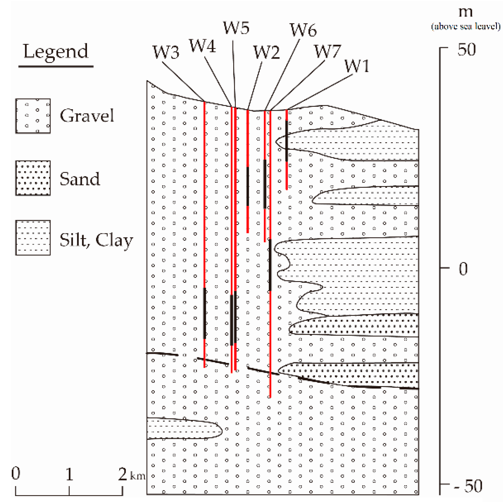
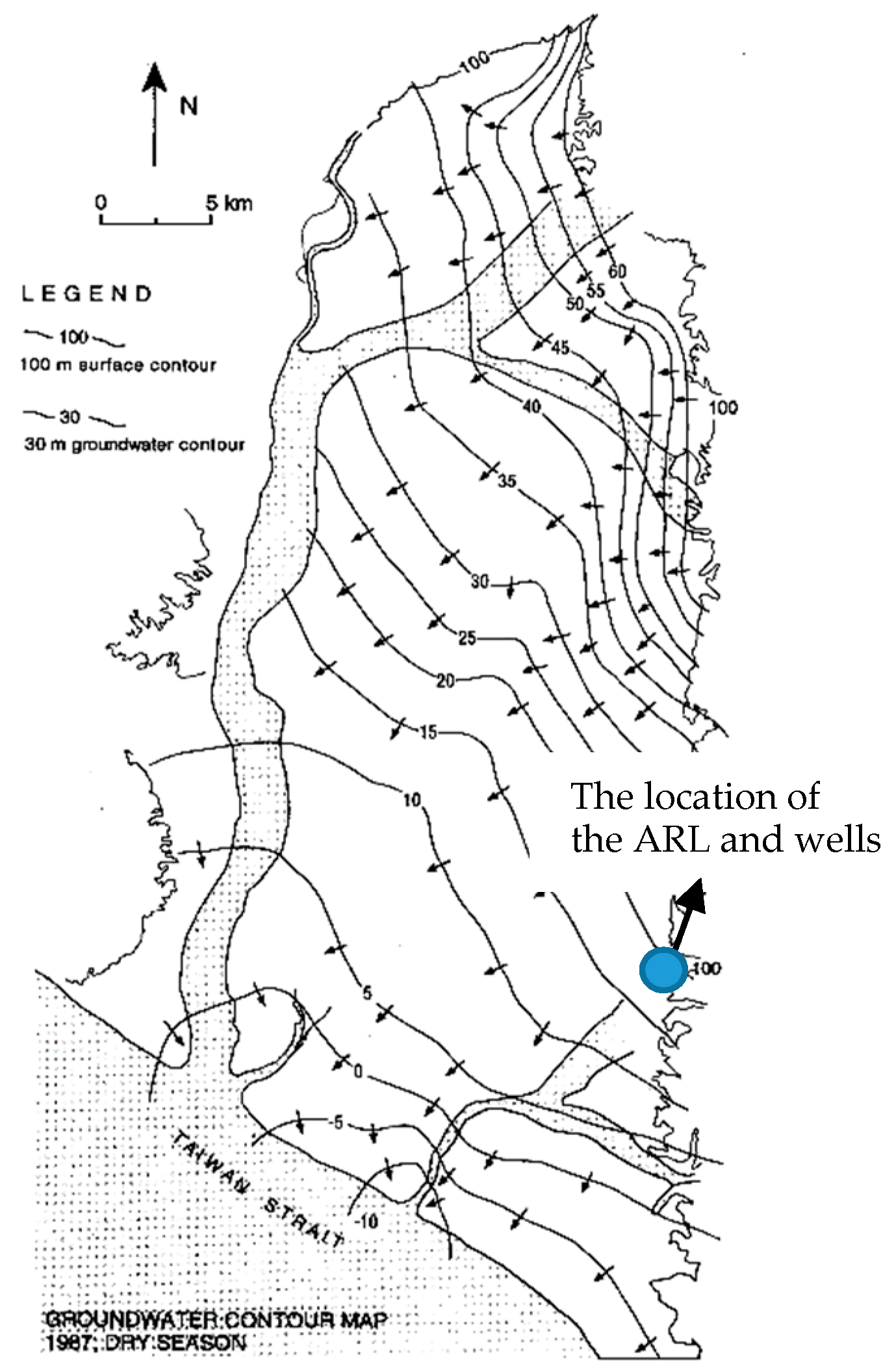
Ting et al. [23] point out that the groundwater catchment in the study area can be divided into three layers, that is, the upper layer, middle layer, and lower layer. The thickness of the upper layer, varying from 10 to 60 m, is assumed to be an unconfined aquifer. The aquifer of the fluvial deposits in the foothills consists of coarse sand and gravel, decreasing in size to sand in a downstream direction with a thickness in excess of 220 m. The middle layer, assumed to be semi-pervious, is a geological formation which has a very low transmissivity compared to the aquifer, with a thickness of about 20 m of clay and sandy clay. The lower layer is assumed to be unconfined in the upper reaches of the area and confined from the mid-fan; the storativity may thus alternate between confined and unconfined values. The aquifers are recharged directly by rainfall, river flow, and subsurface inflow from the northern upstream part of the fluvial fan. The study area is hydraulically bounded in the south by the sea (Taiwan Strait). The screens of each well were all set in the upper layer, which is mainly composed of gravel, and with slice sand, silt, and clay. The transmissivity, storativity, and maximum yield were determined as 9148 m²/day, 6.5 × 10⁻³, and 7084 m³/day, respectively, by the Taiwan Provincial Groundwater Development Bureau [24]. The hydrogeological profile of each well in this study area is redrawn in Figure 3 [25], and the groundwater piezometric map of the Pingtung Plain’s dry season is shown in Figure 4 [26].

The infiltration rate in this study area was evaluated by infiltration experiment in a 30 × 30 × 1.63 m test pit in 2002 [27]. The initial infiltration rate was about 22.76 m/day and the average infiltration rate was 17.26 m/day. After a serial infiltration test, the difference in infiltration rate between 2003 and 2005 had a maximum variation from 15.2 to 10.33 m/day due to the sand addition experiment [28]. If one compares the ARL infiltration result to other studies, the infiltration rate is about 5.9 m/day in the Rokugo Alluvial Fan, Northern Japan [29]; Liu et al.’s study on underground reservoirs in the western suburbs of Beijing estimates the infiltration rate between 1.0 m/day and 3.6 m/day [30].

2.2. Data Collection and Process

For this study, around five years of daily rainfall and daily groundwater table data collected from 2010/05 to 2015/12 were used. Before the model was established, original data underwent a pre-procedure process that included the following steps: (1) rainfall data processing, (2) groundwater table data processing, and (3) data normalization. The data collection and processing procedure steps are described in the following subsections.

2.2.1. Rainfall Data

Mean catchment rainfall can be calculated by several techniques, such as Thiessen polygon, isohyetal, polynomial, geostatistical, inverse distance weighted, multi-quadratic interpolation, and kriging [31,32]. This study referred to Tsou et al. [33] who used the Thiessen polygon method to calculate the mean catchment rainfall. The separated Thiessen’s control area in the Taiwu-1 station was 50.76 km² (15%), in the Xinlaiyi station it was 141.13 km² (40%), and in the Nanhan station it was 156.97 km² (45%). Based on research of the effects of rainfall, rainfall intensity, and groundwater table variation [34], the groundwater table is more sensitive in a five-day time-lag in a shallow layer [35]. Hence, this study combined the rainfall of past 1-day (R1) to past 5-day (R5) and rainfall intensity of past 1-day (RI1) to past 5-day (RI5) as the model inputs.

2.2.2. Groundwater Data

This study referred to Nayak et al. using 2-day groundwater differences as output for the model establishment [17]. In addition, considering the hydrogeology in a shallow groundwater aquifer, the groundwater variation is significantly affected by 10 days of rainfall [36]. Therefore, this study separated rainfall and groundwater data by events, where groundwater table rising past 10 days until groundwater drop was regarded as an event.

2.2.3. Data Normalization

To prevent an error associated with extreme values, data normalization was conducted for the data regarding rainfall, rainfall intensity, and groundwater differences. In addition, this procedure randomized the data using the concept of stochastic statistics to understand the relative change amount in the database. Therefore, the data employed were bounded between 0 and 1 using Equation (1) below, and then they were reverted by following Equation (2) [37]:

$$x_{\mathrm{norm}}=\frac{x-x_{\min }}{x_{\max }-x_{\min }},$$

(1)

$$x=x_{\mathrm{norm}}\times \left(x_{\max }-x_{\min }\right)+x_{\min },$$

(2)

where x_norm is the normalized dimensionless variable, x is the observed value of the variable, x_min is the minimum value of the variable, and x_max is the maximum value of the variable.

2.3. Artificial Neural Network (ANN)

An artificial neural network is an algorithm for processing information by its dynamic state response to inputs. The neural network computes its output at each iteration (epoch) and compares it with the expected output of each input (exemplary) vector in order to calculate the error. An ANN comprises parallel systems that are composed of processing elements (PEs) or neurons, which are assembled in layers and connected through several links or weights. After feeding input data to the input layer, they pass through and are operated on by the network until the output is produced at the output layer. Each neuron receives numerous inputs from other neurons through some weighted connections. These weighted inputs are then summed, and a standard threshold is added, generating the argument for a transfer function (usually linear, logistic, or hyperbolic tangent), which in turn produces the final output of the neuron [38,39].

Hsieh et al. and Liao et al. compared MLP, a time lag recurrent network (TLRN), and a time delay neural network (TDNN) for groundwater simulation in the Lin-Bien River catchment. The MLP model is appropriate and suitable for this study area [40,41]. In order to learn more complex decision functions, inputs are fed into a number of perceptron nodes, each with its own set of weights and threshold [42]. The outputs of these nodes are then inputted into another layer of nodes, and so on. The output of the final layer of nodes is the output of the network. Such a network is termed MLP, and the layers of nodes whose input and output are seen only by other nodes are termed hidden [43]. The connection weights are computed by means of a learning algorithm. There are different variants of back-propagation learning algorithms in the literature [44]. The illustration of the MLP model is shown in Figure 5.

2.4. Sensitivity Analysis (SA)

A sensitivity analysis is a tool for model input importance assessment. Referring to Jha and Sahoo [20] and Memarian et al. [45,46], the SA calculation equation (Equation (3)) is given as follows [47]. When the change is small, the input is less sensitive in the model; on the contrary, when the changes are significant, the input is highly sensitive:

$$S_k=\frac{{\displaystyle \sum _{p=1}^p{\displaystyle \sum _{n=1}^n\left(y_{ip}-\overline{y_{ip}}\right)}}}{{a_k}^2}$$

(3)

where S_k is the sensitivity index for input k, $\overline{y_{ip}}$ is the ith output obtained with the fixed weights for the pth pattern, n is the number of network outputs, p is the number of patterns, and α_k² is the variance of the input k.

3. Results

The ANN model was established using normalized rainfall and groundwater table data. The R² was selected for model performance evaluation. Thus, the sensitivity analysis was conducted to evaluate the importance of the input for the model simulation. All results are discussed below.

3.1. ANN Results

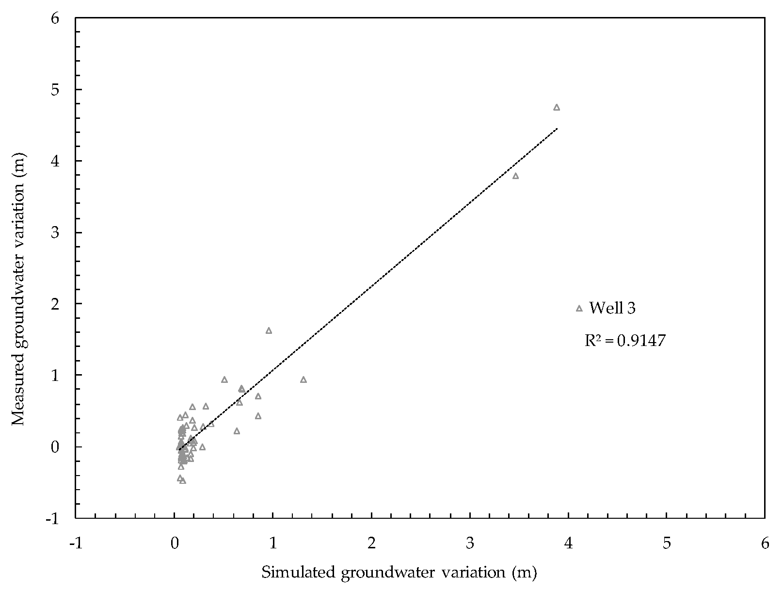
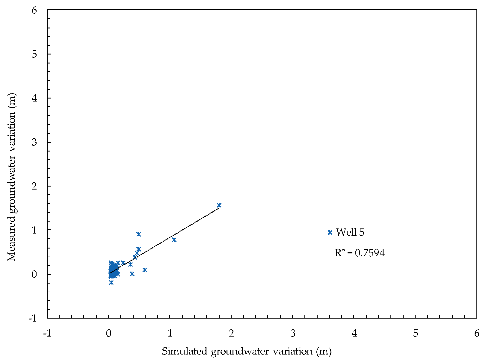
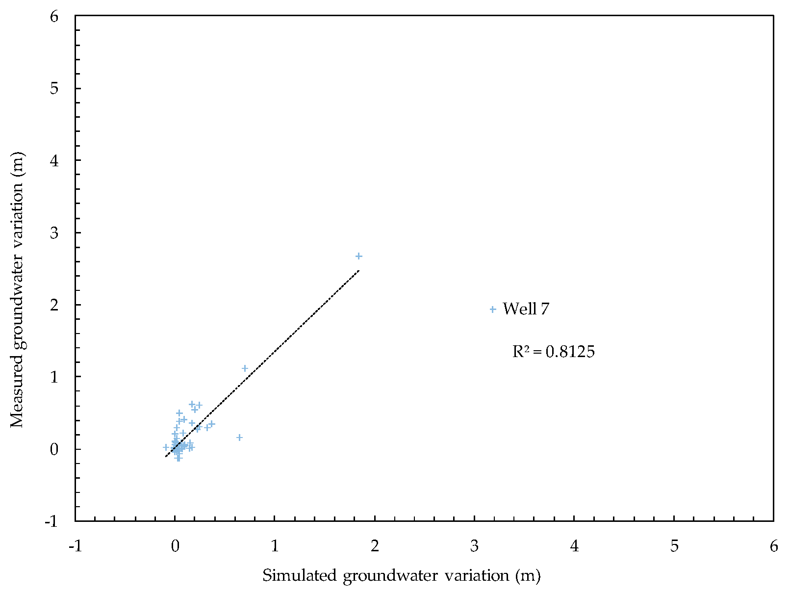
Referring to the training, validation, and testing arrangements from Tayfur and Singh [48], Yang et al. [49] and Memarian et al. [45], respectively, this study used 70% of the data for training, 20% for validation, and 10% for testing. With respect to the PE and hidden layer selection, Cheung et al. suggest 10 PEs in 1 hidden layer [50]. Thus, in this study, PEs were set at 10, and the hidden layer was set at 1. The simulated results revealed that the R² of the MLP model in Well 1 was 0.848, in Well 2 it was 0.854, in Well 3 it was 0.914, in Well 4 it was 0.897, in Well 5 it was 0.759, in Well 6 it was 0.841, and in Well 7 it was 0.812. All MLP model values showed high correlation (R² > 0.8) except for Well 5, which was the farthest well from the Lin-Bien River and the ARL. Comparing Well 5 with a similar location well (Well 6), the well screen of Well 6 (13–25 m, above sea level) was shallower than that of Well 5 (−17 to 5 m, above sea level). The MLP model performance values (R²) are shown in

Table 3. MLP model performance.

Groundwater Monitoring Wells	R2
Well 1	0.848
Well 2	0.854
Well 3	0.914
Well 4	0.897
Well 5	0.759
Well 6	0.841
Well 7	0.812

. The model testing correlation relationship of each well is presented in Figure 6, Figure 7, Figure 8, Figure 9, Figure 10, Figure 11 and Figure 12.

3.2. SA Results

A sensitivity analysis was performed on the MLP model’s simulation results to understand the relative sensitivity of each input to the output. All SA results are shown in

Table 4. Sensitivity analysis index.

Inputs	Well 1	Well 2	Well 3	Well 4	Well 5	Well 6	Well 7
RI5	0.0216	0.0207	0.0163	0.0064	0.0096	0.0049	0.0145
RI4	0.0045	0.0025	0.0035	0.0028	0.0047	0.0133	0.0033
RI3	0.0223	0.0220	0.0156	0.0101	0.0076	0.0002	0.0164
RI2	0.0040	0.0157	0.0231	0.0650	0.0044	0.0102	0.0037
RI1	0.0017	0.0163	0.0130	0.0212	0.0051	0.0021	0.0200
R5	0.0053	0.0132	0.0181	0.0035	0.0238	0.0084	0.0498
R4	0.0203	0.0324	0.0639	0.0029	0.0181	0.0069	0.1489
R3	0.0136	0.0594	0.0343	0.0036	0.0048	0.0036	0.0443
R2	0.0849	0.1095	0.0362	0.0108	0.0030	0.0127	0.0092
R1	0.0102	0.0027	0.0048	0.0173	0.0060	0.0042	0.0372

and Figure 13. Referring to Jha and Sahoo, the level of sensitivity was classified into five categories [20], as shown in

Table 5. Categorization of sensitivity and associated ranks.

Category of Sensitivity	Value of Sensitivity Index	Rank
1. Very high sensitivity	>0.1	1
2. High sensitivity	0.05 to 0.1	2
3. Moderate sensitivity	0.01 to 0.05	3
4. Low sensitivity	0.005 to 0.01	4
5. Very low sensitivity	≤0.005	5

. Based on the value of the sensitivity index for a particular input at the well, the influence level of the model’s sensitivity to the input was ranked on a scale of 1 to 5 (

Table 6. Ranked sensitivity analysis index of each input.

Inputs	Well 1	Well 2	Well 3	Well 4	Well 5	Well 6	Well 7
RI5	3	3	3	4	4	5	3
RI4	5	5	5	5	5	3	5
RI3	3	3	3	3	4	5	3
RI2	5	3	3	2	5	3	5
RI1	5	3	3	3	4	5	3
R5	4	3	3	5	3	4	3
R4	3	3	2	5	3	4	1
R3	3	2	3	5	5	5	3
R2	2	1	3	3	5	3	4
R1	3	5	5	3	4	5	3

). The sensitivity analysis indicated that, for past 5-day rainfall and rainfall intensity, R2 and RI3 were the highest and second highest sensitivities in Well 1; in Well 2, the results were R2 and R3; in Well 3, they were R4 and R2; in Well 4, they were RI2 and RI1; in Well 5, they were R5 and R4; in Well 6, they were RI4 and R2; and in Well 7, they were R4 and R5. The rainfall (R) is more sensitive than rainfall intensity (RI) in this research area. The highest and second highest sensitivities are listed in

Table 7. Highest and 2nd highest sensitivities.

Groundwater Monitoring Wells	Highest Sensitivity		2nd Highest Sensitivity
	Index	Variable	Index	Variable
Well 1	2	R2	3	RI3
Well 2	1	R2	2	R3
Well 3	2	R4	3	R2
Well 4	2	RI2	3	RI1
Well 5	3	R5	3	R4
Well 6	3	RI4	3	R2
Well 7	1	R4	3	R5

(if the ranked result in the same value, the original SA index was compared).

When considering the SA results and the information in the location map of the study area (Figure 2), one can see that Wells 1 to 3 are within the study catchment, which is adjacent to Lin-Bien River and the ARL, and responded faster in R1, R2, R3, RI1, RI2, RI3, respectively; Wells 4 to 7 are outside the catchment and far from the ARL; R4, R5, RI4, RI5 were found to be sensitive in Wells 5 to 7. It can be concluded that the groundwater table variation adjacent to the Lin-Bien River and the ARL is response-related with rainfall time-lag. It is worth noting that, although Well 4 is located outside the catchment, it still has a certain degree of sensitivity from past 3-day rainfall (R1, R2, R3, RI1, RI2, RI3, respectively), the reason for which is discussed below.

The sensitivity of each well is influenced by the well screen position. The reason for past 3-day rainfall (R1, R2, R3, RI1, RI2, RI3, respectively) being sensitive in Well 4 is that the well screen’s location is similar to the one in Well 3. After considering the SA results about the information for each groundwater monitoring well (Table 2), it was observed that 2-day rainfall (R1, R2, RI1, RI2, respectively) was more sensitive due to the well screen location being above sea level, for example, in Wells 1, 2, and 6.

4. Discussion

The purpose of this study was to discover the highly sensitive variables of a groundwater simulation model adjacent to an ARL using short-term rainfall. The model was established by MLP with past 10-day short-term events. Normalized rainfall (R1 to R5), rainfall intensity (RI1 to RI5), and groundwater data were selected as model variables. The R² was used for model accuracy assessment [18]. A sensitivity analysis (SA) was conducted to evaluate the importance of each model input. The study results are discussed as follows.

First, during the model establishment, the MLP model was suggested for development [5,40,41]. The best fit R² of the MLP model was 0.914 (Well 3) and the lowest R² in MLP was 0.759 (Well 5). This model uses rainfall as an input; the rainfall converges in the ARL and the river then infiltrates into the groundwater layer. The farthest well (Well 5) from the Lin-Bien River and the ARL responded more slowly than the other wells with a lower R². Comparing Well 5 with a similar location well (Well 6), the well screen of Well 6 (13–25 m, above sea level) was shallower than that of Well 5 (−17 to 5 m, above sea level). Therefore, the rainfall response in Well 6 was faster than in Well 5.

Second, a sensitivity analysis was conducted for input importance evaluation. The highest and second highest inputs in Well 1 were R2 and RI3; in Well 2, they were R2 and R3; in Well 3, they were R4 and R2; in Well 4, they were RI2 and RI1; in Well 5, they were R5 and R4; in Well 6, they were RI4 and R2; and in Well 7, they were R4 and R5. The rainfall amount (R) was more sensitive than rainfall intensity (RI) in this research area.

Finally, when considering the SA results for the Lin-Bien River catchment area (Figure 2) and the relevant hydrogeological profile (Figure 3), a slight difference between “within the catchment” and “outside the catchment” can be found. Wells 1 to 3 are in the study catchment and adjacent to Lin-Bien River and the ARL, and responded faster in past 3-day rainfall (R1, R2, R3, RI1, RI2, RI3, respectively) than the other four wells. On the other hand, R4, R5, RI4, RI5 were found to be sensitive in Wells 5 to 7. Although Well 4 was located outside the catchment, it still had a certain degree of sensitivity from past 3-day rainfall (R1, R2, R3, RI1, RI2, RI3, respectively) because the location of its well screen was similar to the one in Well 3. Moreover, R2 was highly sensitive due to the well screen being located above sea level, that is, Wells 1, 2, and 6. It can be concluded that the groundwater table variation in this study area is response-related with the distance from the wells to the river and the ARL, and the rainfall time-lag.

5. Conclusions

A sensitivity analysis is not only a tool for the input importance evaluation of a groundwater simulation model, but it is also a useful method, considered with a hydrogeological map and geological characteristics, for explaining influences on the physical mechanism of groundwater infiltration, taking into account the complexity of the relevant physical groundwater model’s development. This SA study is helpful to researchers wishing to study related ARL efficiency issues.

References

1. Peng, T.R.; Lu, W.C.; Chen, K.Y.; Zhan, W.J.; Liu, T.K. Groundwater-recharge connectivity between a hills-and-plains’ area of western Taiwan using water isotopes and electrical conductivity. J. Hydrol. 2014, 517, 226–235. [Google Scholar] [CrossRef]
2. Wang, C.H.; Kuo, C.H.; Chang, F.C. The Changing Face of the Groundwater Environment in Taiwan. Bull. Cent. Geol. Surv. 2004, 17, 1–22. [Google Scholar]
3. T.W.R.A. Taiwan Water Usage Annual Report; Taiwan Water Resources Agency, Ministry of Economic Affairs: Taipei, Taiwan, 2017; p. A-14.
4. T.W.R.A. Taiwan Groundwater Withdrawal and Pumping. Available online: https://www.wra.gov.tw/6950/7170/7356/7488/13319 (accessed on 14 July 2019).
5. Liao, F.L. Using Artificial Neural Network for Estimating the Effects on Groundwater from Artificial Recharge or Rainfall. National Pingtung University of Science and Technology: Pingtung County, Taiwan, 2017. [Google Scholar]
6. T.P.W.C.B. Compilation and Analysis of Existing Groundwater and Subsidence Data of Taiwan II–the Pingtung Plain; Ministry of Economic Affairs: Taipei, Taiwan, 1994.
7. T.P.W.C.B. Study on the Improvement of the Groundwater Monitoring System in the Pingtung Plain; Ministry of Economic Affairs: Taipei, Taiwan, 1998.
8. Ineson, J. Hydrogeological and Groundwater Aspects of Artificial Recharge. In Proceedings of the Artificial Groundwater Recharge Conference, England, UK, 21–24 September 1970; pp. 1–14. [Google Scholar]
9. Muckel, D. Artificial Recharge in Relation to Groundwater Storage. In Proceedings of the Annual Conference on Water for Texas, College Station, TX, USA, 16–18 September 1958; pp. 85–94. [Google Scholar]
10. Walton, W.C. Groundwater Resource Evaluation. In McGraw-Hill Series in Water Resources and Environmental Engineering (USA) eng; McGraw-Hill: New York, NY, USA, 1970. [Google Scholar]
11. Morbidelli, R.; Saltalippi, C.; Flammini, A.; Cifrodelli, M.; Picciafuoco, T.; Corradini, C.; Govindaraju, R. Laboratory investigation on the role of slope on infiltration over grassy soils. J. Hydrol. 2016, 543, 542–547. [Google Scholar] [CrossRef]
12. Morbidelli, R.; Corradini, C.; Saltalippi, C.; Flammini, A.; Dari, J.; Govindaraju, R. A New Conceptual Model for Slope-Infiltration. Water 2019, 11, 678. [Google Scholar] [CrossRef]
13. Chen, C.T.; Chen, L.S.; Huang, J.Y.; Huang, S.J. A Study on Ground Water Level Forecasting by Combining Neural Networks and Semi-variogram Model. J. Taiwan Agric. Eng. 2015, 61, 14–28. [Google Scholar] [CrossRef]
14. Coppola, E.A., Jr.; Rana, A.J.; Poulton, M.M.; Szidarovszky, F.; Uhl, V.W. A neural network model for predicting aquifer water level elevations. Groundwater 2005, 43, 231–241. [Google Scholar] [CrossRef] [PubMed]
15. Yu, H.-L.; Lin, Y.-C. Analysis of space–time non-stationary patterns of rainfall–groundwater interactions by integrating empirical orthogonal function and cross wavelet transform methods. J.Hydrol. 2015, 525, 585–597. [Google Scholar] [CrossRef]
16. Daliakopoulos, I.N.; Coulibaly, P.; Tsanis, I.K. Groundwater level forecasting using artificial neural networks. J. Hydrol. 2005, 309, 229–240. [Google Scholar] [CrossRef]
17. Nayak, P.C.; Rao, Y.S.; Sudheer, K. Groundwater level forecasting in a shallow aquifer using artificial neural network approach. Water Resour. Manag. 2006, 20, 77–90. [Google Scholar] [CrossRef]
18. Sahoo, S.; Jha, M.K. Groundwater-level prediction using multiple linear regression and artificial neural network techniques: A comparative assessment. Hydrogeol. J. 2013, 21, 1865–1887. [Google Scholar] [CrossRef]
19. Liu, L.W.; Hsieh, S.H.; Chung, W.G.; Wang, Y.M. Sensitivity Analysis on the Rising Relation of Short-term Rainfall and Unconfined Aquifer Groundwater Table. In Proceedings of the 2017 4th International Conference on Coastal and Ocean Engineering (ICCOE 2017), Osaka, Japan, 29 March 2017; p. 64. [Google Scholar]
20. Jha, M.K.; Sahoo, S. Efficacy of neural network and genetic algorithm techniques in simulating spatio-temporal fluctuations of groundwater. Hydrol. Process. 2015, 29, 671–691. [Google Scholar] [CrossRef]
21. Ahlawat, R. Hydrological Data Network Modelling Using Artificial Neural Network in Betwa Catchment. Int. J. Soft Comput. Eng. (IJSCE) 2014, 3, 132–134. [Google Scholar]
22. Ting, C.S.; Kerh, T.; Liao, C.J. Estimation of groundwater recharge using the chloride mass-balance method, Pingtung Plain, Taiwan. Hydrogeol. J. 1998, 6, 282–292. [Google Scholar] [CrossRef]
23. Ting, C.S.; Zhou, Y.; Vries, J.D.; Simmers, I. Development of a Preliminary Ground Water Flow Model for Water Resources Management in the Pingtung Plain, Taiwan. Groundwater 1998, 36, 20–36. [Google Scholar] [CrossRef]
24. T.P.W.C.B. Investigation Report on Ground Water Resources of the Pingtung Plain; Ministry of Economic Affairs: Taichung, Taiwan, 1961.
25. Ministry of Economic Affairs. Geological Sensitive Groundwater Recharge Area Delineation Plan-G0002 Pingtung Plain; Ministry of Economic Affairs: Taipei, Taiwan, 2014.
26. Ting, C.S. Groundwater Resources Evaluation and Management for Pingtung Plain, Taiwan. Ph.D. Thesis, Vrije Universiteit, Amsterdam, The Netherlands, 1997. [Google Scholar]
27. C.T.C.I. Pingtung County Water Resources Development and Conservation of The Overall Planning and Lin-Bien River Upstream Artificial Lake Engineering Project Settings–Groundwater Recharge Field Test Report; Pingtung County Government: Pingtung, Taiwan, 2000; pp. 3–23.
28. Tu, Y.-C.; Ting, C.-S.; Tsai, H.-T.; Chen, J.-W.; Lee, C.-H. Dynamic analysis of the infiltration rate of artificial recharge of groundwater: A case study of Wanglong Lake, Pingtung, Taiwan. Environ. Earth Sci. 2011, 63, 77–85. [Google Scholar] [CrossRef]
29. Hida, N.; Ishikawa, E.; Ohta, Y. Experimental Study of Basin Artificial Recharge of Ground Water in Rokugo Alluvial Fan, Northern Japan. J. Groundw. Hydrol. 1999, 41, 23–33. [Google Scholar] [CrossRef] [Green Version]
30. Liu, J.X.; Cai, Q.S. Research on the Groundwater Reservoir in the West Suburb of Beijing; Geological Publishing Company: Beijing, China, 1988. [Google Scholar]
31. Abo-Monasar, A.; Al-Zahrani, M.A. Estimation of rainfall distribution for the southwestern region of Saudi Arabia. Hydrol. Sci. J. 2014, 59, 420–431. [Google Scholar] [CrossRef] [Green Version]
32. Ewea, H.A.; Elfeki, A.M.M.; Bahrawi, J.A.; Al-Amri, N.S. Sensitivity analysis of runoff hydrographs due to temporal rainfall patterns in Makkah Al-Mukkramah region, Saudi Arabia. Arab. J. Geosci. 2016, 9, 424. [Google Scholar] [CrossRef]
33. Tsou, I.; Chen, C.N.; Wang, Y.M.; Kuo, Y.C. A Simulation Study for Flood Disaster Reduction by Detention Pond in Lin-Bian River Basin. In Proceedings of the International Conference on Disaster Management, Kumamoto, Japan, 25 August 2012; pp. 399–406. [Google Scholar]
34. Bogaard, T.A. Analysis of Hydrological Processes in Unstable Clayey Slopes. Ph.D. Thesis, Utrecht University, Utrecht, The Netherlands, 2001. [Google Scholar]
35. Jasmin, I.; Murali, T.; Mallikarjuna, P. Statistical analysis of groundwater table depths in upper Swarnamukhi River basin. J. Water Resour. Prot. 2010, 2, 577. [Google Scholar] [CrossRef]
36. Apps, J.A.; Zheng, L.; Spycher, N.; Birkholzer, J.T.; Kharaka, Y.; Thordsen, J.; Kakouros, E.; Trautz, R. Transient changes in shallow groundwater chemistry during the MSU ZERT CO2 injection experiment. Energy Procedia 2011, 4, 3231–3238. [Google Scholar] [CrossRef]
37. Wang, Y.-M.; Elhag, T.M. An adaptive neuro-fuzzy inference system for bridge risk assessment. Expert Syst. Appl. 2008, 34, 3099–3106. [Google Scholar] [CrossRef]
38. Talebizadeh, M.; Morid, S.; Ayyoubzadeh, S.A.; Ghasemzadeh, M. Uncertainty analysis in sediment load modeling using ANN and SWAT model. Water Resour. Manag. 2010, 24, 1747–1761. [Google Scholar] [CrossRef]
39. Traore, S.; Wang, Y.M.; Chung, W.G. Predictive accuracy of backpropagation neural network methodology in evapotranspiration forecasting in Dédougou region, western Burkina Faso. J. Earth Syst. Sci. 2014, 123, 307–318. [Google Scholar] [CrossRef]
40. Hsieh, S.H.; Chung, W.G.; Wang, Y.M. Using Artificial Neural Networks for Groundwater Table in Unconfined Aquifer Forecasting. In Proceedings of the 2017 4th International Conference on Coastal and Ocean Engineering (ICCOE 2017), Osaka, Japan, 29 March 2017; p. 63. [Google Scholar]
41. Liao, F.L.; Liu, L.W.; Chung, W.G.; Wang, Y.M. Using ANN for modeling the unconfined groundwater table variation induced by artificial recharge lake in dry season. In Proceedings of the 2017 4th International Conference on Coastal and Ocean Engineering (ICCOE 2017), Osaka, Japan, 29 March 2017; p. 98. [Google Scholar]
42. Bishop, C.M. Neural Networks for Pattern Recognition; Oxford University Press: New York, NY, USA, 1995. [Google Scholar]
43. Lippmann, R.P. An introduction to computing with neural nets. IEEE Assp Mag. 1987, 4, 4–22. [Google Scholar] [CrossRef]
44. Hagan, M.T.; Demuth, H.B.; Beale, M.H.; De Jesús, O. Neural Network Design; Pws Pub.: Boston, MA, USA, 1996; Volume 20. [Google Scholar]
45. Memarian, H.; Balasundram, S.K.; Tajbakhsh, M. An expert integrative approach for sediment load simulation in a tropical watershed. J. Integr. Environ. Sci. 2013, 10, 161–178. [Google Scholar] [CrossRef] [Green Version]
46. Memarian, H.; Bilondi, M.P.; Rezaei, M. Drought prediction using co-active neuro-fuzzy inference system, validation, and uncertainty analysis (case study: Birjand, Iran). Theor. Appl. Climatol. 2016, 125, 541–554. [Google Scholar] [CrossRef]
47. Principe, J.C.; Euliano, N.R.; Lefebvre, W.C. Neural and Adaptive Systems: Fundamentals through Simulations; Wiley: New York, NY, USA, 2000; Volume 672. [Google Scholar]
48. Tayfur, G.; Singh, V.P. ANN and fuzzy logic models for simulating event-based rainfall-runoff. J. Hydraul. Eng. 2006, 132, 1321–1330. [Google Scholar] [CrossRef]
49. Yang, C.T.; Marsooli, R.; Aalami, M.T. Evaluation of total load sediment transport formulas using ANN. Int. J. Sediment Res. 2009, 24, 274–286. [Google Scholar] [CrossRef]
50. Cheung, S.O.; Wong, P.S.P.; Fung, A.S.; Coffey, W. Predicting project performance through neural networks. Int. J. Proj. Manag. 2006, 24, 207–215. [Google Scholar] [CrossRef] [Green Version]
Figure 1. Location map of Pingtung Plain, after [22].
Water 11 01704 g001
Figure 2. Location map of the study area (W1 to W7 is Well 1 to Well 7, respectively).
Water 11 01704 g002
Figure 3. Hydrogeological profile of the study area (W1 to W7 is Well 1 to Well 7, respectively), after [25]. The A-A’ profile of Figure 1.
Water 11 01704 g003
Figure 4. Groundwater piezometric map of the Pingtung Plain’s dry season (November to May) [26].
Water 11 01704 g004
Figure 5. Illustration of the multilayer perception (MLP) model, after [39].
Water 11 01704 g005
Figure 6. The model testing correlation relationship of Well 1.
Water 11 01704 g006
Figure 7. The model testing correlation relationship of Well 2.
Water 11 01704 g007
Figure 8. The model testing correlation relationship of Well 3.
Water 11 01704 g008
Figure 9. The model testing correlation relationship of Well 4.
Water 11 01704 g009
Figure 10. The model testing correlation relationship of Well 5.
Water 11 01704 g010
Figure 11. The model testing correlation relationship of Well 6.
Water 11 01704 g011
Figure 12. The model testing correlation relationship of Well 7.
Water 11 01704 g012
Figure 13. Sensitivity index of each input of the MLP model.
Water 11 01704 g013