Article

Assessment of the Impact of Sand Mining on Bottom Morphology in the Mekong River in An Giang Province, Vietnam, Using a Hydro-Morphological Model with GPU Computing

1
Faculty of Marine Resource Management, Ho Chi Minh City University of Natural Resources and Environment, 236B Le Van Sy Street, Ward 1, Tan Binh District, Ho Chi Minh City 700000, Vietnam
2
Institute for Environment and Resources, 142 To Hien Thanh Street, Ward 14, District 10, Ho Chi Minh City 700000, Vietnam
3
School of Electrical and Computer Engineering, Ulsan National Institute of Science and Technology (UNIST), 50 UNIST -gil, Ulju, Eonyang, Ulsan 44919, Korea
4
Department of Fluid Mechanics, Ho Chi Minh City University of Technology, 268 Ly Thuong Kiet Street, Ward 14, District 10, Ho Chi Minh City 700000, Vietnam
5
Vietnam National University Ho Chi Minh City, Linh Trung Ward, Thu Duc District, Ho Chi Minh City 700000, Vietnam
6
Department of Computer Science and Engineering, College of Informatics, Korea University, Seoul 02841, Korea
7
Institute for Computational Science and Technology, SBI building, Quang Trung Software City, Tan Chanh Hiep Ward, District 12, Ho Chi Minh City 700000, Vietnam
*
Author to whom correspondence should be addressed.
Water 2020, 12(10), 2912; https://doi.org/10.3390/w12102912
Submission received: 26 August 2020 / Revised: 15 October 2020 / Accepted: 15 October 2020 / Published: 18 October 2020
(This article belongs to the Section Water Erosion and Sediment Transport)

Abstract

:
Sand mining, among the many activities that have significant effects on the bed changes of rivers, has increased in many parts of the world in recent decades. Numerical modeling plays a vital role in simulation in the long term; however, computational time remains a challenge. In this paper, we propose a sand mining component integrated into the bedload continuity equation and combine it with high-performance computing using graphics processing units to boost the speed of the simulation. The developed numerical model is applied to the Mekong river segment, flowing through Tan Chau Town, An Giang Province, Vietnam. The 20 years from 1999 to 2019 is examined in this study, both with and without sand mining activities. The results show that the numerical model can simulate the bed change for the period from 1999 to 2019. By adding the sand mining component (2002–2006), the bed change in the river is modeled closely after the actual development. The Tan An sand mine in the area (2002–2006) caused the channel to deviate slightly from that of An Giang and created a slight erosion channel in 2006 (−23 m). From 2006 to 2014, although Tan An mine stopped operating, the riverbed recovered quite slowly with a small accretion rate (0.25 m/year). However, the Tan An sand mine eroded again from 2014–2019 due to a lack of sand. In 2014, in the Vinh Hoa communes, An Giang Province, the Vinh Hoa sand mine began to operate. The results of simulating with sand mining incidents proved that sand mining caused the erosion channel to move towards the sand mines, and the erosion speed was faster when there was no sand mining. Combined with high-performance computing, harnessing the power of accelerators such as graphics processing units (GPUs) can help run numerical simulations up to 23x times faster.

1. Introduction

Sand is an essential resource in the construction and maintenance of river delta surfaces. In the process of increasing urbanization, the demand for extensive construction material is becoming a concern for infrastructure. To meet the demands for construction material, several sand mines on the river have been operating and have produced many impacts on the environment and river morphology [1,2,3,4,5]. Numerous studies have demonstrated that sand mining in alluvial rivers causes disturbances within geomorphic processes, bottom revolutions, and their functions [2,4,6]. Removing a large volume of sediment alters the hydraulic properties of the flow and the morphodynamic evolution of the riverbed [6,7,8,9,10].
The Mekong River is the 10th largest river in the world, with a basin of about 795,000 km2 in size and about 4800 km in length. The main portion of the Mekong River flows through six countries including China, Myanmar, Thailand, Laos, Cambodia, and Vietnam. [11]. The lower Mekong morphology is created by bedrock-controlled and alluvial reaches [12]. There are many causes of continuous and severe erosion in the area, such as excessive sand mining and sediment imbalances leading to erosion [13,14]. The annual extraction, according to the estimation of Bravard et al. (2013), is 34 Mm3 (approximately 54 MT/year for an aggregate density of 1.6 t/m3), featuring mostly (90%) sand and, to a smaller degree, gravel (8%) and pebbles (1%). This utilization is focused on mining in Cambodia (21 MT/year), Vietnam (8 MT/year), Thailand (5 MT/year), and Laos (1 MT/year) [15]. It has been estimated that sand mining has removed 200 Mm3 of bedload since 1998. Hackney’s research indicated that sand in the Mekong riverbed is minimal and that sand transport to the delta is under threat from increased bed sediment extraction [16]. The total sand flux entering the Mekong delta (6.17 MT/year ± 2.01 MT/year) is far less than the current sand extraction rates (50 MT/year). As a result, it takes only 10 to 18 years to scour the riverbed sufficiently at these current rates to change the riverbed and sediment transport [17].
In a geological survey study along the Tien River, the characteristics of the Tien Riverbed in Hong Ngu, An Long, Sa Dec, Mo Cay, Ben Tre, and Ba Tri were shown to be clay (d < 0.0015 mm), while Tan Chau and My Thuan were characterized by clay mud (0.0015 < d < 0.003 mm) [18]. Compared with the Hjulstrom–Sundborg diagram, a flow with a velocity higher than 0.005 m/s is capable of carrying moving particles from 0.002 to 0.075 mm, and if the speed is higher than 0.3 m/s–0.4 m/s, the sediment particles with the above dimensions are likely to be separated from the bottom by the flow [19]. Currently, 11 sand mines are operating in An Giang area according to Decision No. 1697/QĐ–UBND on 18 July 2018, An Giang Province. The voids created by the mining (the pits themselves and the incised channels) trap sediment transported into the reach from upstream, reducing sediment loads downstream of the pit, thereby inducing incision from the flow. This matter leads to bed changes in the river [20].
Many studies have used numerical models to simulate sediment transport and bed changes, including MIKE ([21,22], DELFT [23], TELEMAC [24,25], CCHE 2,3D [26,27]. In general, these studies focus on explaining the current situation. However, for the effects under the scenarios of flow and sediment changes, there is no research demonstrating the impact of sand mining on the bottom changes in this area. Moreover, in these studies, the hydrodynamic model is the primary tool. A model was developed by our team and successfully applied to several other regions, including the Mekong Delta. Bay et al. (2018) simulated the litho-dynamic processes and bottom morphology in the coastal area, such as the flow, sediment transport, and bed changes for Can Gio and Cua Lap, Vietnam [28,29]. This model is based on the Reynolds equation system coupled with the sediment transport and bedload continuity equations [6,10,30,31,32,33,34]. The authors applied the above model to calculate the bottom changes for the waters of Can Gio and Cua Lap. The results from the model prove that the calculations and developments are suitable in reality. In 2019, the authors improved the hydraulic model with a roughness coefficient that changes with the bed level. Moreover, the alluvial boundary condition at the liquid boundary in the sediment transport module was developed using a characteristic line, allowing sediment to move out of the computational area. Thus, the movements of suspended sediments and the bottom transport in the near-boundary area are more accurate. The study area in this research was a part of the Tien River that flows through the Tan Chau area of the Mekong Delta [35]. However, the results were still inaccurate compared to reality due to sand exploitation in the area.
For bed change due to sand mining, Binoy Aliyas Mattamana (2013) studied the transportation of sand in the river using numerical modeling and applied sand inflow to Periyar River, India. The present study deals with Meyer-Peter‘s equations to estimate bedload transport. However, this study only focused on calculating the sand flow to the sand mine area to assess the recovery time of the sand mine. The amount of sand lost due to exploitation and riverbed evolution during sand mining has not been studied [36]. Other sand mining studies also focused on assessing the impact of the sand mining concept on river hydrodynamics [37] and environmental water quality [38,39].
In another respect, although simulations of the morphological changes and other hydrodynamic phenomena can be modeled via partial differential equations, this method is implicitly impractical due to the large temporal and spatial grid. Hence, it is not possible to solve within a certain amount of time [40,41,42,43,44,45]. In the 15th Pacific Conference on Computer Graphics and Applications, the United States, Wu and Eftekkarian (2011) emphasized that reducing the calculation speed and improving in-situ visualization will be necessary for integration hydrodynamic models [45,46,47].
Our primary motivation for this improvement is that in the current era of high-performance computing, numerous multi-core co-processors can help accelerate simulation processes at different scales (Intel MIC, Graphics Processing Units) in which the data are laid out as a rectilinear grid. There is little or no dependency between the results of the current and other time steps. At present, increasingly more artificially intelligent applications whose core components are neural networks are using graphics processing units (GPUs) to accelerate their training and inference phases. Specifically, we developed our numerical model using NVIDIA Compute Unified Device Architecture (CUDA) C/C++ to reduce the timing execution of the simulation. This library helps our code communicate with the GPUs’ parallel processing units (physical threads) via the abstraction of CUDA logical threads.
Based on the above analysis, in this paper, we proposed a sand mining component for the numerical model established by Bay et al. [35] to achieve the most accurate bottom evolutions. Furthermore, the numerical model is combined with high-performance computing using graphics processing units. The objectives of this study are as follows:
(1)
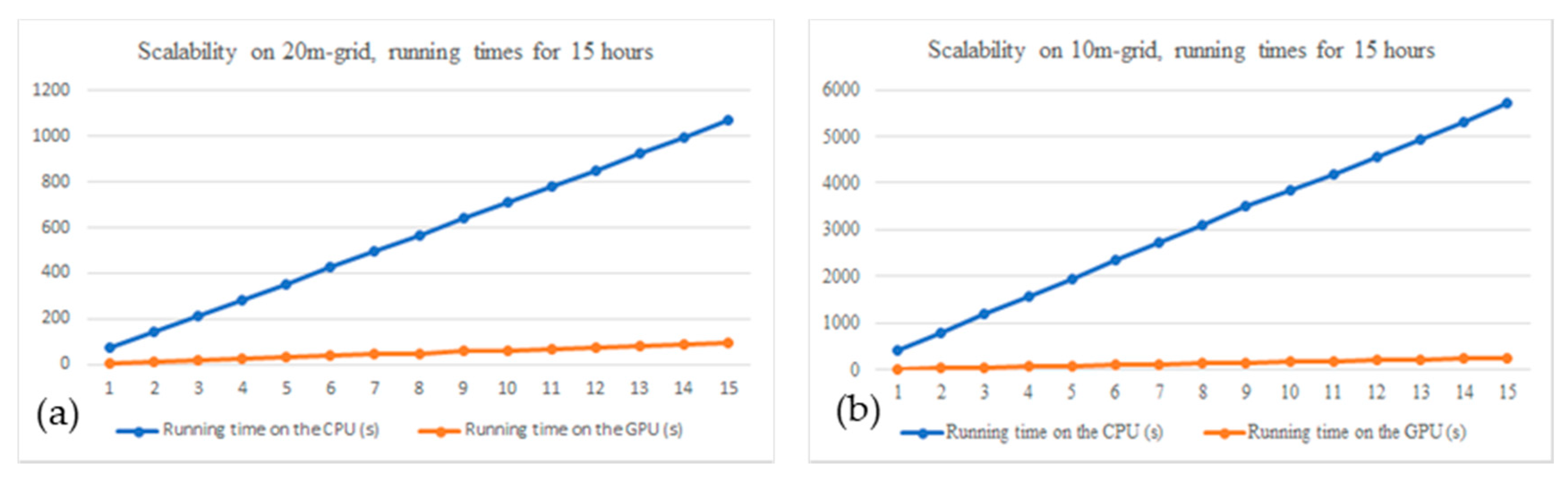
First, the computational times on a single-core CPU machine are too slow to meet the simulation’s on-demand requirements. We thus parallelize our solver using massively multi-core GPUs to accelerate the computing speed, which is evaluated with a strong-scaling factor.
(2)
Second, we assess the changes in bottom morphology in the Mekong River in An Giang province under sand mining.

2. Materials and Methods

2.1. Study Area

The study area is a segment about 17 km long, flowing through An Giang, Dong Thap, and belongs to Mekong Delta, Vietnam (Figure 1). The segment has the style of a braided river, the riverbed is widened, and there are sandbars in the heart. This section has complex terrain, stream folding, and substantial erosion. Additionally, this area has exploited the excessive sand at near river bank, causing complicated bed changes and effecting the An Giang embankment.
The Mekong River Basin has complex geology resulting from plate tectonics and their activities [20,48]. Mekong’s average discharge to the sea is about 15,000 m3/s, with a predictable 20-fold seasonal fluctuation from the dry season (November–June) to the wet season (July–October) [12,20].
In this area, there are two sand mines, including Tan An (2002–2006) and Vinh Hoa (2014–2019). The Tan An sand mine was invested in by Vinh An Private Enterprise (An Giang). This mine operated from 2002 to 2006; its annual output is 200,000 m3, and its mining area is 91 ha [49]. From 2014 until the present, the Vinh Hoa mine has operated (According to License No. 04/GP-UBND 23 April 2013) with an annual output of 200,000 m3 and a mining area of 27.9 ha.

2.2. Numerical Model

This model is based on a system of four governing equations averaged according to depth as follows. In particular, the ς-axis is facing up, and the standard “0” is placed on the static surface, as shown in Figure 2.

2.2.1. Reynolds Equation in the Ox and Oy Directions

u t + u u x + v u y = g ς x K u u 2 + v 2 h + ς + A 2 u
v t + u v x + v v y = g ς y K v u 2 + v 2 h + ς + A 2 v
ς t + x [ ( h + ς ) u ] + y [ ( h + ς ) v ] = 0
The model adopted is a 2D surface model where Ox and Oy represent the study area’s length and width.

2.2.2. Suspended Sediment Transport Equation

C t + γ v ( u C x + v C y ) = 1 H x ( H K x C x ) + 1 H y ( H K y C y ) + S H
where S in this equation stands for the erosion and deposition rates (m/s).
The source S is defined after Van Rijn [51] with three different states:
When τb > τe, S = E (Erosion rate):
E = M ρ s τ b τ e τ e
When τb < τd, S = D (Deposition rate):
D = ω s m C b τ d τ b τ d
When τeτbτd:
S = 0

2.2.3. Bed Load Continuity Equation with Sand Mining Component:

h t = 1 1 ε p [ ( S + S s m ) + x ( H K x C x ) + y ( H K y C y ) + q b x x + q b y y ]
Here, Ssm is the sand mine source and the standing sand mining rate (m/s).
In this paper, the sand component is integrated into the bed load continuity equation. After sand mining, sand is removed from the calculation area; hence, Ssm is not involved in the suspended sediment transport equation. Sand mining will stop when the bottom elevation reaches the government’s permitted mining level, where qb = (qbx, qby).
These equations are solved by the Alternating Direction Implicit (ADI) method. The ADI method’s central concept is to split different finite equations into two: one with the x-derivative and the other with the y-derivative, both taken implicitly [52].

2.3. Graphics Processing Unit (GPU)

In the current era of high-performance computing, numerous multi-core co-processors can help accelerate the simulation processes at different scales (Intel MIC, Graphics Processing Units) where the data are laid out as a rectilinear grid. There is little or no dependency between the results of the current and other time steps. Presently, increasingly more artificially intelligent applications whose core components are neural networks make use of GPUs to accelerate their training and inference phases. Programming such accelerators requires a medium to interact with the physically parallel cores that handle the data. For example, Intel MIC and ATI GPUs can be accelerated by Open Computing Language (OpenCL); NVIDIA GPUs ship with NVIDIA CUDA C/C++. In particular, these libraries/programming languages help our code communicate with the parallel processing units of GPUs (physical threads) via the abstraction of logical threads. Running our numerical model on GPUs can reduce the timing execution of simulation. We chose to implement our model on NVIDIA GPUs since these GPUs achieve higher Floating Point Operation Per Second (FLOP) when dealing with numerically precise data. NVIDIA GPU schedulers help map many logical threads to many (but limited) physical threads with zero-cost. In other words, switching between the connections of logical and physical threads will not waste time and energy. In NVIDIA GPUs, the logical threads are laid out in warps, blocks, and grids (in a coarse-to-fine manner). Each warp contains 32 threads, and each block can hold a maximum of 1024 threads. All of the threads in the same block are scheduled to be executed concurrently, and all 32 threads in the same warp are designed to run a set of instructions simultaneously. This is why GPUs can support running a program in parallel with many computational operations (i.e., an embarrassingly parallel workload).
A computational algorithm such as the above numerical model is a procedure in which each step is a correctly defined state and executed by computers. For a given problem, multiple algorithms are commonly used to solve it. Some may require a lower computational cost than others. Some may allow execution in parallel at a larger scale than others; some are more stable, and some require less memory consumption. Unfortunately, no solution satisfies all of the above four criteria. Given a problem and a list of constraints to run that problem, we usually have to choose a direction to compensate for the above four aspects under a specific physical hardware system. Some algorithms have certain advantages/disadvantages in maintaining certain numerical precisions. In contrast, others have to sacrifice accuracy to scale up the solution to handle big data such as our hydrological data.
The theoretical solution for this 2D hydrological problem is common to use Finite Difference Methods (FDM) with the ADI scheme. At the first half of the time step, our computational model starts to scan the grid along the horizon to compute the velocity u and the depth ς implicitly, and then explicitly solves for the velocity ν. Similarly, at the second half of the time step, the model scans the grid along the vertical axis to compute the velocity ν and the depth ς implicitly. Explicitly, the model applies the FDM to numericalize the equation and rearrange variables; it will then form a system of linear equations (more concretely, a tridiagonal linear system). Some numerical solvers for this, such as the Thomas algorithm [53], include a forward scan and a backward substitution. However, there are more dependencies in this algorithm that hinder its full parallelization. Therefore, leveraging the Thomas algorithm for solving tridiagonal linear systems for our problem is simple but cannot exploit the massive parallelism of a GPU or a GPU’s high memory bandwidth. Various algorithms have been developed to parallelize banded matrix solvers [53]. After examining different parallel matrix solvers, we decided to adopt the parallelized Thomas algorithm with data marshaling, developed in [54] with open source code provided in [55]. To avoid memory transfer from the device to the host, we exploit a CUDA feature called dynamic parallelism, where the device kernels can be launched from other kernels. By parallelizing the Thomas algorithm and performing data marshaling, we achieved a higher level of parallelism and higher memory bandwidth, increasing the performance significantly.
The Alternating Direction Implicit (ADI) scheme is known to be naturally suitable for parallelization, since, in each sweep, each row/column can be scanned independently. Therefore, each row or column can be assigned to one thread to be solved individually. However, due to the GPU’s hierarchical memory, the computation needs to be distributed into small chunks to process the tridiagonal linear system. Hence, there are many more optimization steps in programming design strategies to access different levels of GPU memories, such as the local registers, shared memory, cache, and global memory. By exploiting these, we reduced the computational overhead from the data movement in between the GPU memories and improved the performance of the GPU cores.

3. Setting up the Model

3.1. Study Area Mesh

The topography was collected from the Department of Investment and Construction Project of Tan Chau town area on 6 October 1999 at The Southern Institute Of Water Resources Research in 2006 and 2014 and from the “Research to identify causes, mechanisms and propose feasible technical and economical solutions to reduce erosion, sedimentation for the Mekong river system (2017–2020)” project, code No. KHCN-TNB.ĐT/14-19/C10, in 2019.
The features (water level ς(t), discharge Q(t), and total suspended sediment C(t)) at Tan Chau station were collected from 1999 to 2019 (Figure 1). The study area has two boundaries whose features were identified based on their correlation function (f(ς), f(Q), f(C) with Tan Chau station. Measurement data were taken from the boundaries of the “Research to identify causes, mechanisms and propose feasible technical and economical solutions to reduce erosion, sedimentation for the Mekong river system (2017–2020)” project, code No. KHCN-TNB.ĐT/14-19/C10, from 10:00on 6 June 2018 to 10:00 on 13 June 2018.
The study area mesh is a rectangular grid with 981 × 845 elements, including the land and riverbed, with Δx = Δy = 10 m for the whole region. Sand mine sources were added to the model by matrices Ssm(i, j) (as Figure 3), in which Ssm(i, j) is the sand mining rate at i, j cells (the locations of these sand mines are described in Figure 1). The sand mining rate at the i, j cell corresponding to scenarios (SC1, SC2A, SC2B, SC3, SC4A, SC4B), the annual output, the square of Tan An, and the Vinh Hoa sand mines, is outlined in Table 1.
The speed and location of the sand mining of Tan Chau and Vinh Hoa sand mines are shown in Figure 3:

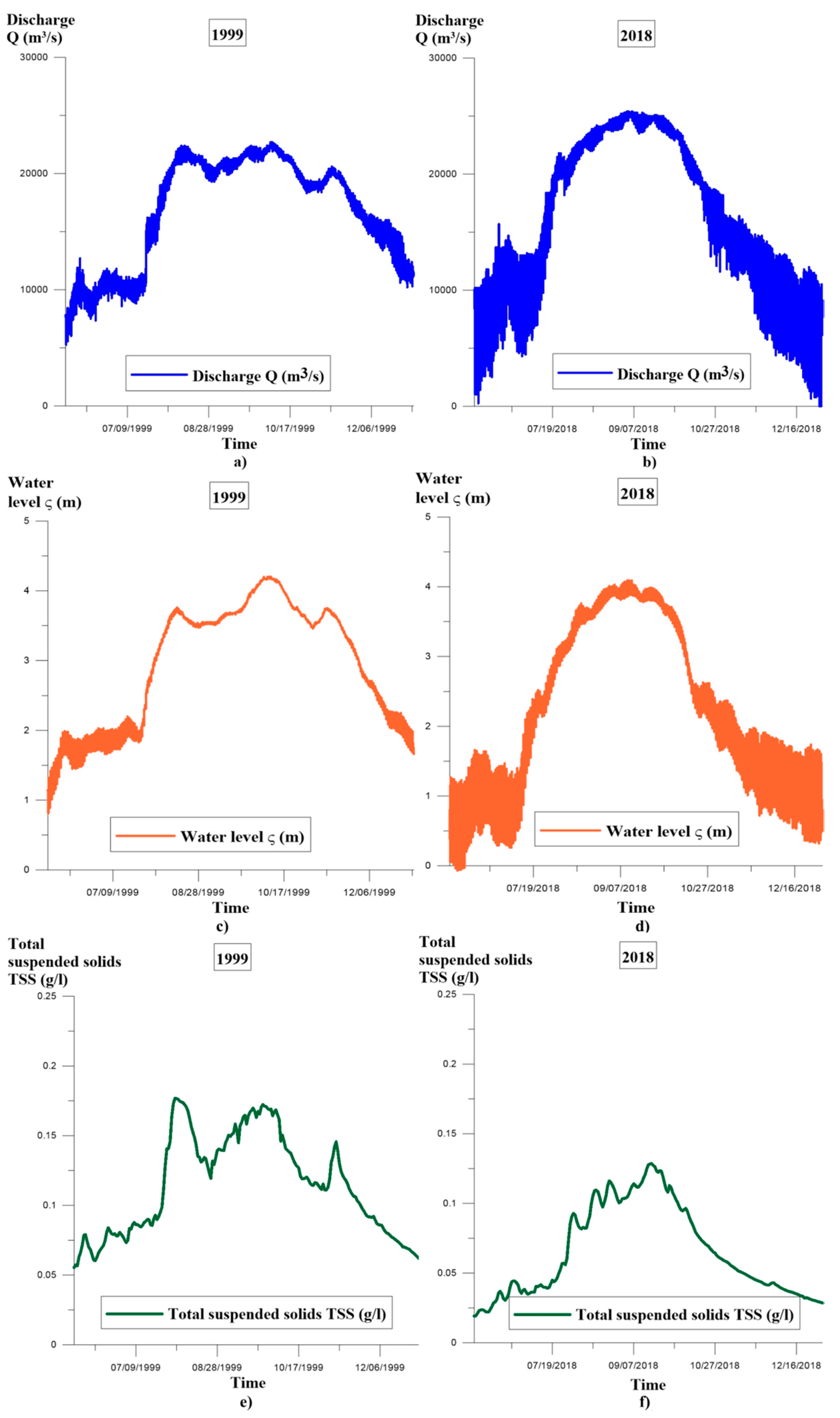
3.2. Initial and Boundary Conditions

3.2.1. Initial Conditions

In the model, if starting from t0 = 0, the hydraulic module is tied to a static state (Figure 2), and the sediment transport module is set to an initial constant basal concentration. Where the problem is calculated from a time t = t1, the initial condition will be the velocity fields u, ν (x, y), and concentration C (x, y) at time t1 across the computational domain.

3.2.2. Boundary Conditions

The Open Boundary

Hydrodynamics conditions:
The upstream boundary is Q(t), from Q(t), the velocity recalculated as follows [56]:
u , v =   [ Q   ( h i 5 3 ) h i 5 3 h i Δ x ]  
Furthermore, because up and down the fluctuations of the water levels vary from time to time (and due to the moving boundaries problem (flooding and drying fronts)), the study area is classified into calculation grid cells. The depth in each element/cell was monitored, and the elements were classified as dry, partially dry, or wet.
The downstream boundary: ς(t).
Sediment transport conditions:
When water flows into the computational domain, C = Co.
In cases where the flow flows out of the domain, C is calculated through the advective transport process (where the diffusion process is ignored), solved by the characteristic line method [35]. By this method, sediment is loaded in and out of the calculation area, making the simulation results more accurate.

Solid Wall Boundary

Hydrodynamics conditions: un = 0
Sediment transport conditions: C n p = 0
For the calibration and validation model, the location of the calibration is Tan Chau station. In this model, the calibration time is 1999, and 2018 (7-day measurement data from 10:00 6 June 2018 to 10:00 13 June 2018) is the validation time. The input data, including flow Q(t), water level ς(t), and sediment concentration C(t) for 1999 and 2018, are shown in Figure 4. The sediment boundary downstream is not used for the model because it flows out of the domain.

4. Results and Discussion

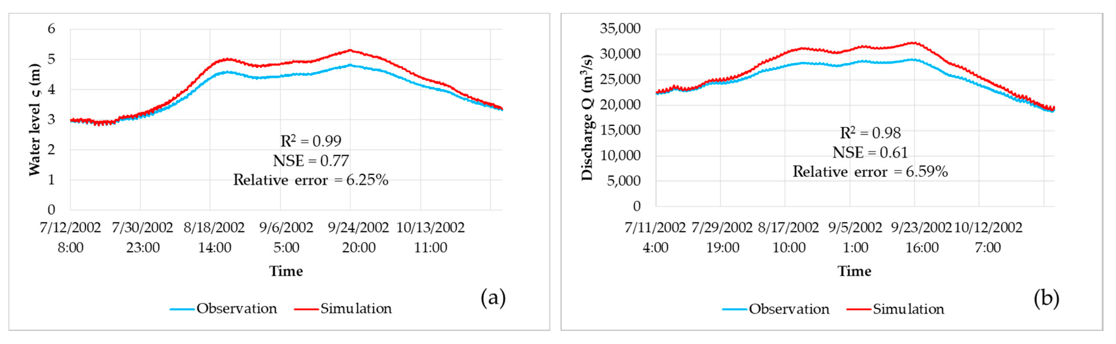
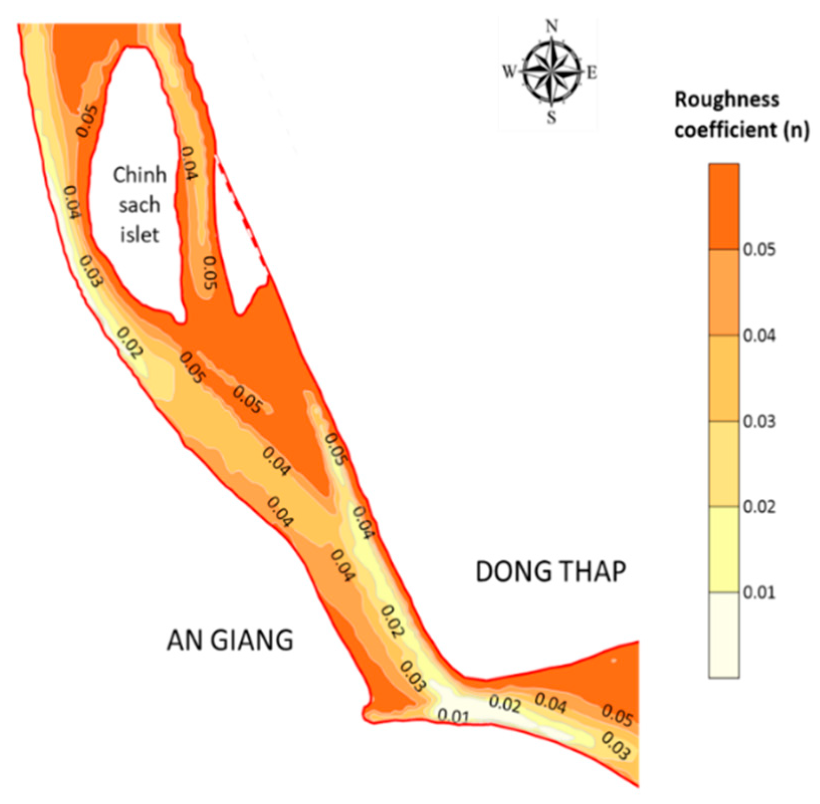
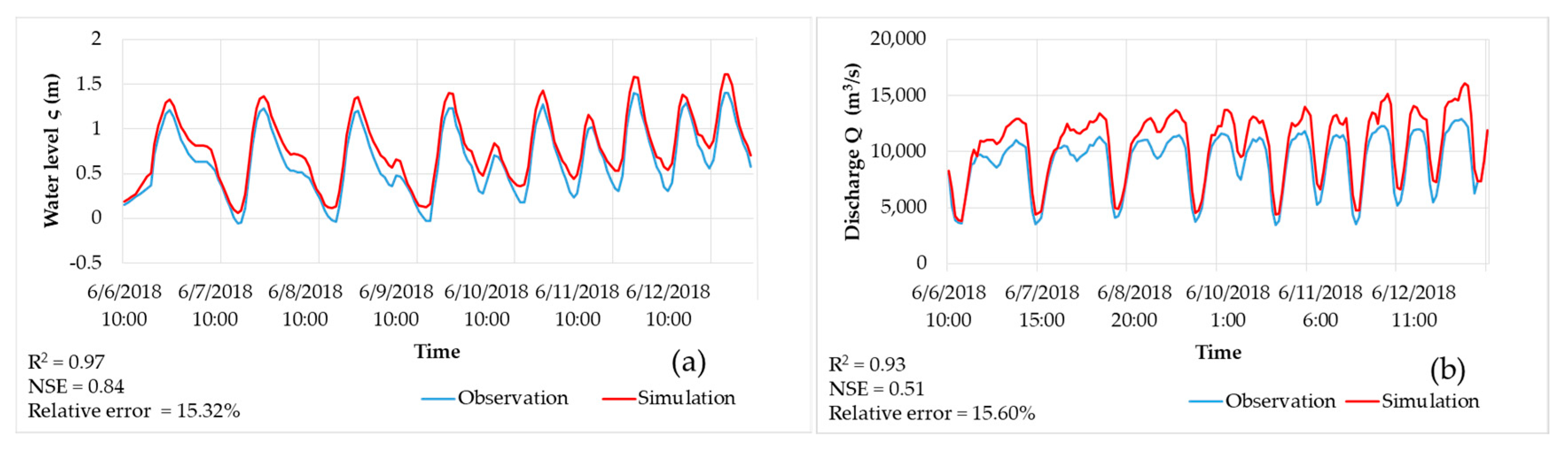
4.1. Calibration and Validation

4.1.1. Hydraulic Model

To calibrate and validate the models, as well as for comparison purposes, the Nash–Sutcliffe efficiency coefficient (NSE) and the coefficient of determination (R2) were used to measure the model performance [57,58,59].
The verification parameter in this model is the roughness coefficient, which was changed in inverse proportion to the water depth. The calibration results show that there was little difference between the simulation results and measurements of the discharge and water level at Tan Chau station between the observation and simulation results from 11 July 2002 to 30 July 2002 (Figure 5). The graphical results during calibration indicated adequate calibration and validation across the range of discharge and water levels. However, the calibration results of the water level showed a better match than those of the discharge. The NSE values for the calibration of discharge and the water level reached 0.61 and 0.77, respectively, while the R2 values were 0.98 and 0.99. According to Moriasi’s research [59], these values indicate that the hydraulic model performance achieved outstanding values. Thus, it is believed that the hydrodynamic model is well-calibrated and that the predicted results are close to actual water movements.
The roughness coefficient was recorded after calibration with a range of 0.055 from 0.005 to 0.06 corresponding to the bed level, varying from 41 to 0.1 m. During the experimental process, n2 (0.003) corresponding to h2 (25 m) was found to make the roughness coefficient in the study area more suitable. Hence, the roughness value is changed from 0.005 to 0.03 when the bed level ranges from 0.1 to 25 m and from 0.003 to 0.06 when the bed level ranges from 25 to 41 m.
Below is a rough map for the first 500 h starting on 15 May 1999 in Figure 6. Consequently, the roughness coefficient in the domain was computed, as shown based on the bed level at that time.
After calibration, the model was validated against 7-day measurement data from 10:00 6 June 2018 to 10:00 13 June 2018. Similar to the calibration, although the calibration result of the water level showed a better match than those of discharge (Figure 7), the evaluation criteria values were also very good for both features. While NSE values were 0.92 and 0.98 for discharge and water level, the R2 values were 0.99 for both these features.

4.1.2. Sediment Transport Model

Similar to the hydraulic model, the sediment transport simulation was calibrated and validated for the two periods from 11 July 2002 to 30 October 2002 and for the 7-day measurement data from 10:00 6 June 2018 to 10:00 13 June 2018. According to evaluation criteria values, the sediment transport model achieved excellent results in terms of the sediment concentration for calibration and validation, with 0.67 and 0.52 for the NSE values and 0.96 and 0.81 R2 values. The graphical results during calibration and validation at Tan Chau station are shown in Figure 8.
After calibration and validation, numerous studies have applied bed parameters such as dispersion, critical shear stress for deposition, and acute shear stress for the erosion of bed layers to simulate the processes of sediment transportation, erosion, and deposition [60]. In this study, these parameters were used for calibrating the sediment simulation. The most relevant parameters in the model are summarized in Table 2.

4.2. Improved Computing Speed When Combining GPUs

We conducted the experiment by directly comparing the accuracy, running times, and the scalability of the proposed solution with and without GPUs. Our computational workstation was as follows: Intel i7 7000 CPU, 16 GB RAM, equipped with an NVIDIA Titan V GPU 12 GB VRAM. Consequently, running in the same environment will produce a direct and fair comparison and a concise result for acceleration (Figure 9 and Figure 10).
As can be seen from Figure 11, the results obtained from the CPU (drawn by Surfer) and GPU versions (drawn by an in-situ Python script) align with each other and thus guarantee the correctness of the model (the source of error from numerical precision is considered insignificant). Moreover, the running times of the simulations (Table 3) show that harnessing the power of GPUs can accelerate performance from 10 to 25 times.
In this subsection, we explain and discuss the methodology that parallelizes the new programming language of CUDA C/C++ using GPUs to accelerate the simulation of 2D hydrological models. We chose and combined multiple CPUs approaches and usedc current state-of-the-art tridiagonal linear system solvers on the GPU to achieve the same results within a shorter period of time in both coarse and fine grid decomposition. The results clearly show that leveraging GPU acceleration can accommodate complex grids in a large-scale manner.

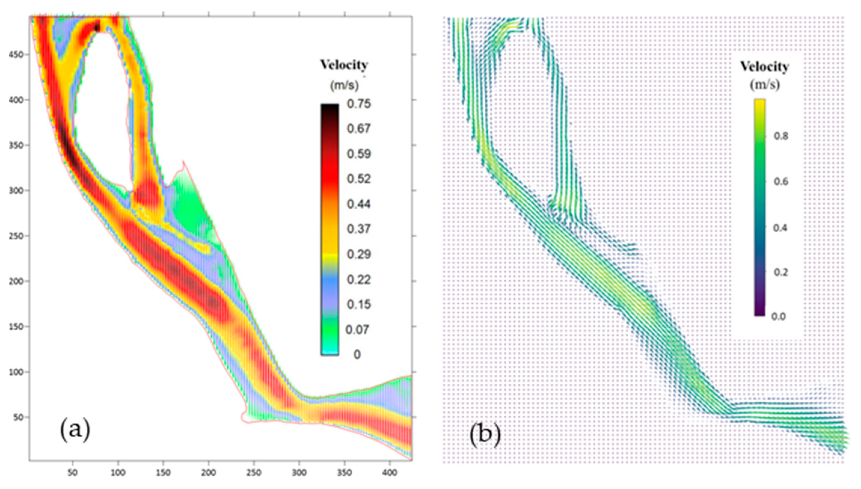
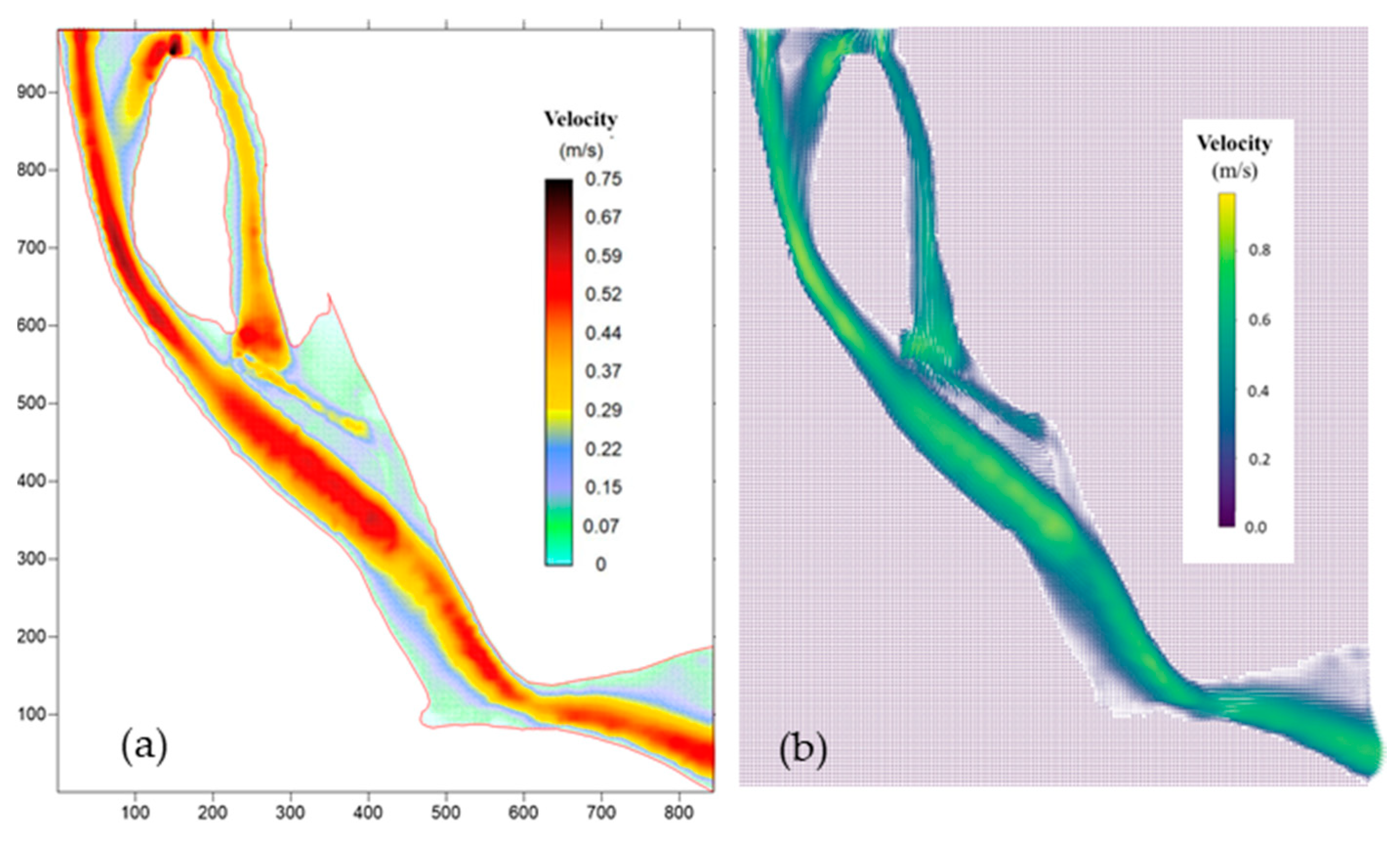
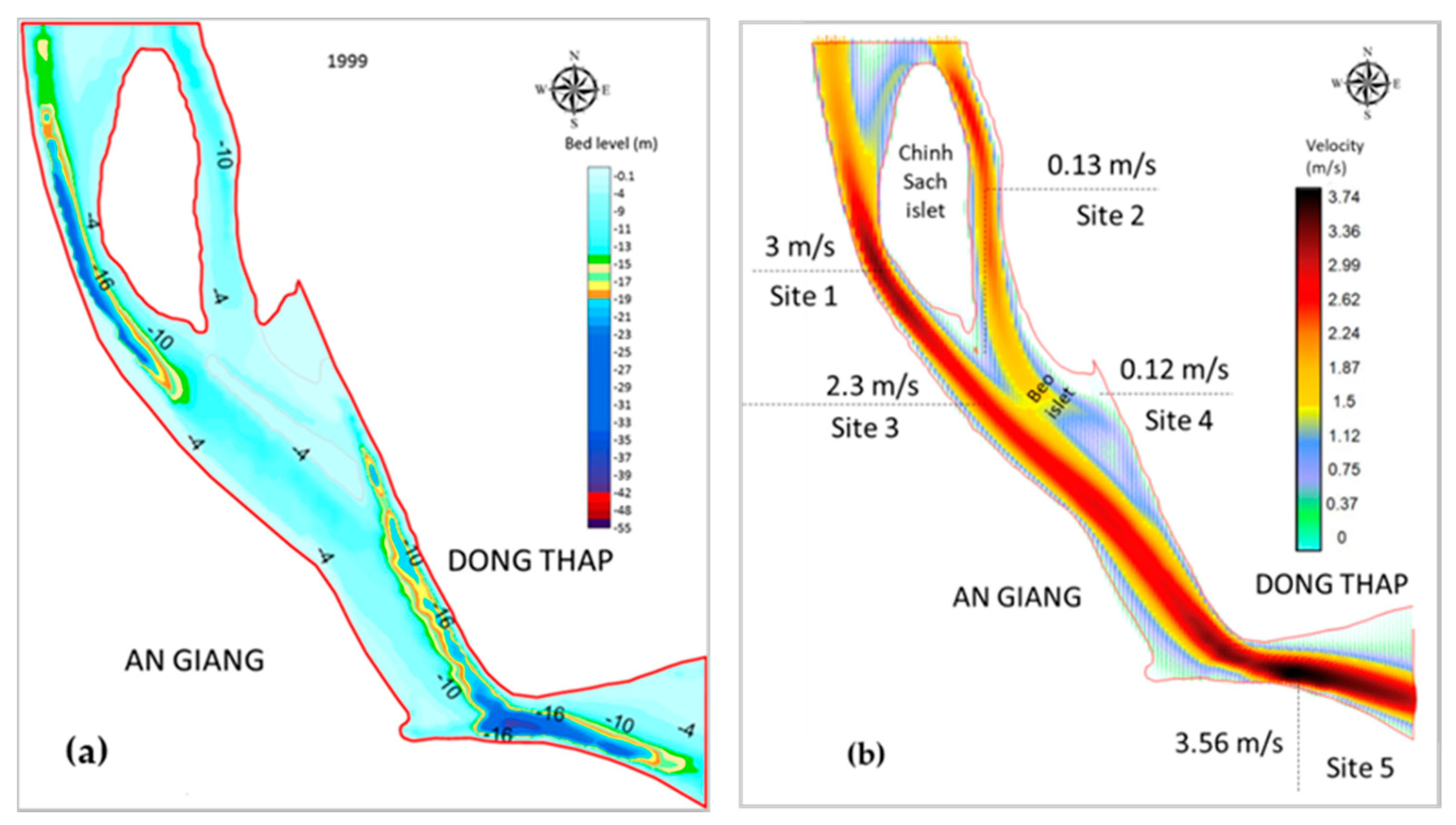
4.3. The Hydraulic Simulation of the Tien River Segment in Mekong Delta

The simulation period for this study was continuous from 1999 to 2019. A velocity field of the peaking flood at 21:00 on 29 September 2002 was extracted, as shown in Figure 12.
The velocity field results of the peaking flood at 21:00 on 29 September 2002 show that the following:
At site 1 (Figure 12), due to a combination of initially deep terrain (−12 m) and the suddenly narrowing section compared to the upstream section, the velocity of the flow was quite large (about 3 m/s). The conflux flow after passing through Chinh Sach islet tended to push towards An Giang (about 2.3 m/s, at site 2). The velocity at the position of the policy tail (site 3) was relatively small (0.13 m/s), which is smaller than the deposition speed of the sediment particles at the Tien river segment (about 0.34 m/s) [19], so this position tended to accrete.
Similarly, at the tail of the mudflat on the Dong Thap side (at site 4), the bathymetry was quite shallow (about −1 m). When the flow velocity was small (0.12 m/s), the sediment particle was deposited gradually, leading to the mudflat being widened.
At the curved section (site 5), there was a combination of a narrowed curved flow and a deep erosion pit, so the flow velocity here was very large (about 3.56 m/s) leading to severe bed erosion.

4.4. Results of Bottom Changes and Analysis

According to the bottom changes in the study area calculated from 1999 to 2019, four scenarios happened in reality, as follows:
  • SC1: From 1999 to 2002 was the time before the sand mines started operating.
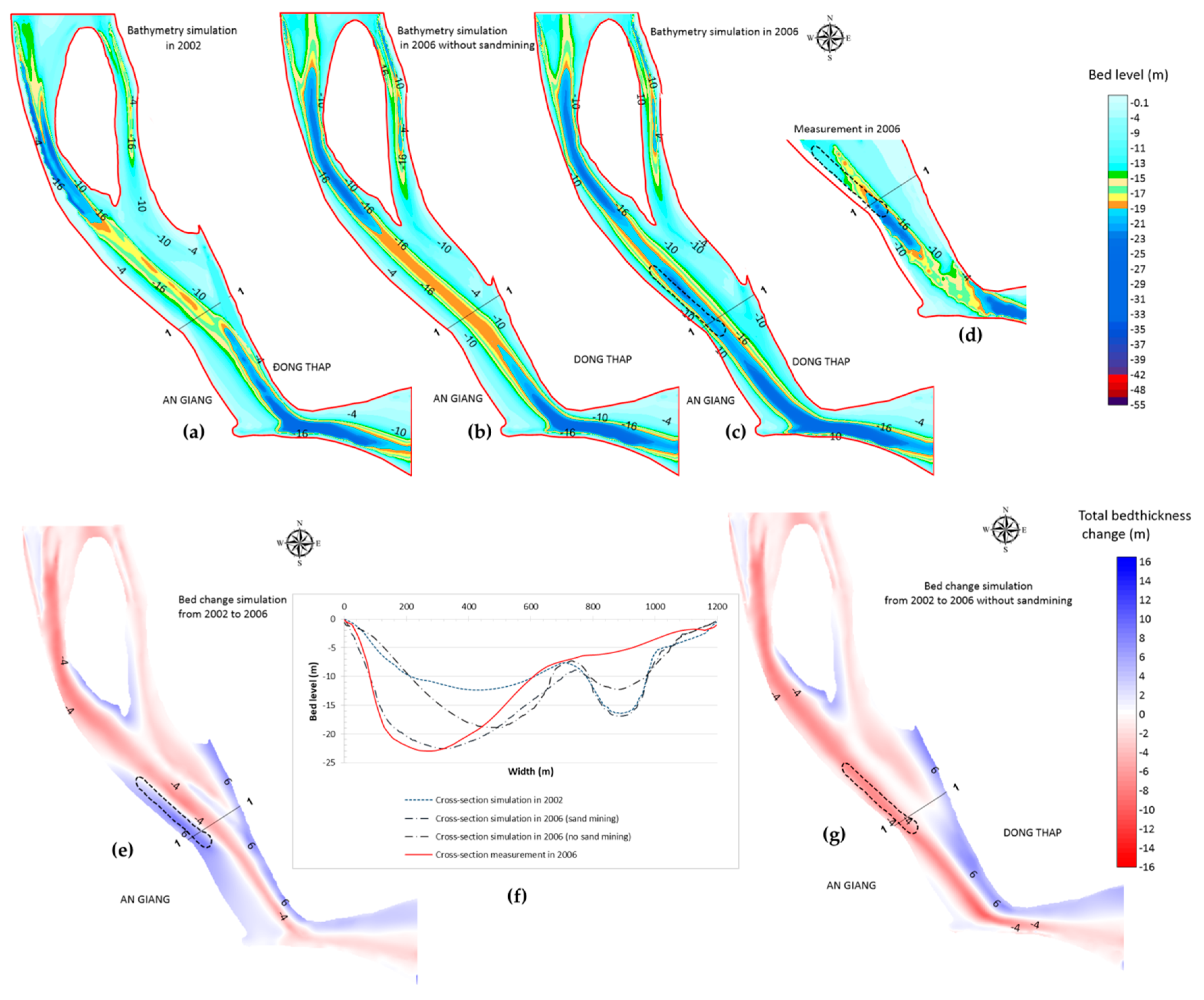
  • SC2A: From 2002 to 2006 was the time that Tan An sand mine was in operation.
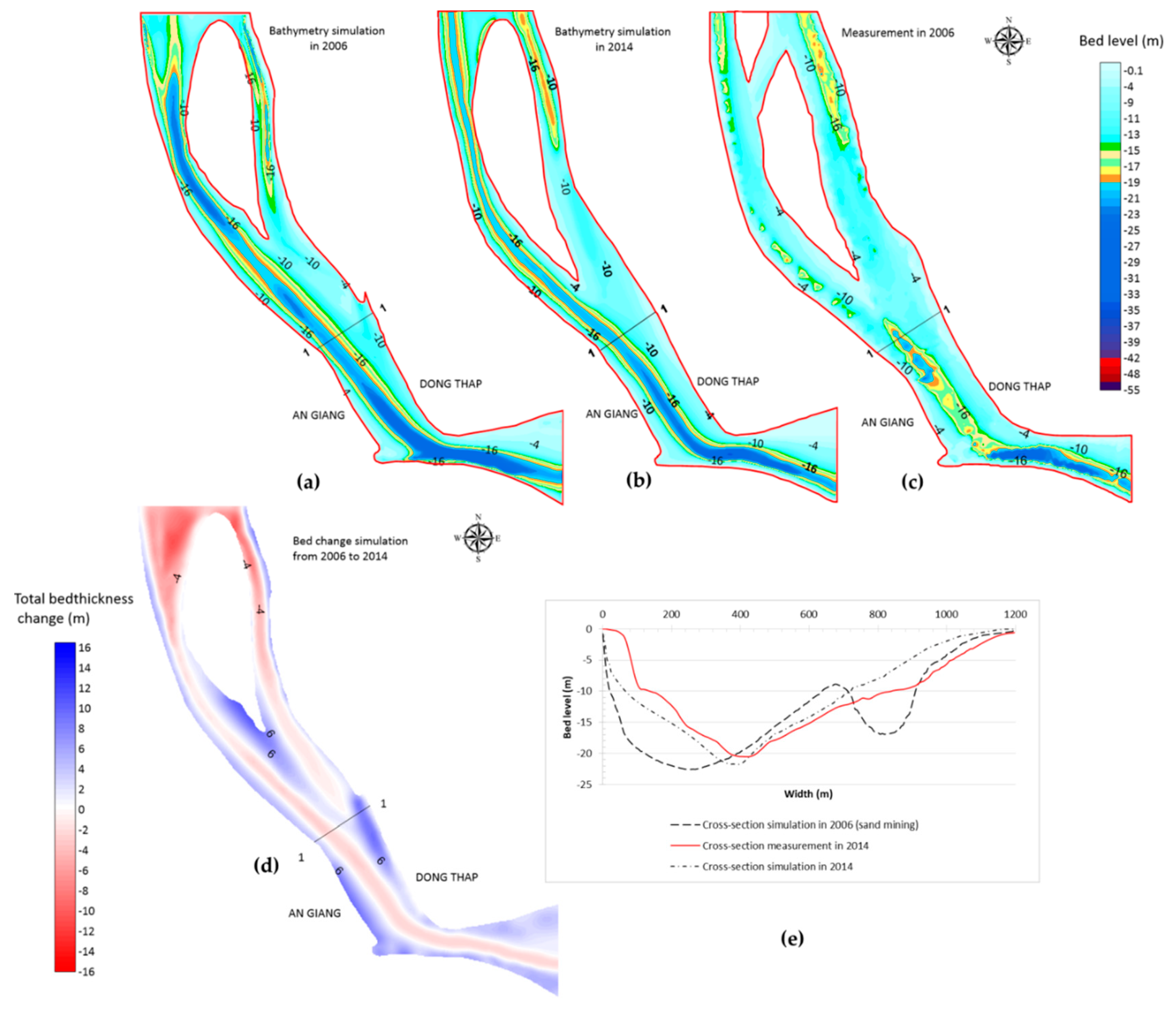
  • SC3: From 2006 to 2014, there was no sand quarry in the study area.
  • SC4A: From 2014 to 2019, the Vinh Hoa sand mine is in operation.
To facilitate assessment of the impact of the sand mining of the Tan An and Vinh Hoa sand mines on the riverbed, we calculated two additional scenarios:
  • SC2B: From 2002 to 2006, there was no sand mining at Tan An sand mine.
  • SC4B: From 2014 to 2019, there was no sand mining at Vinh Hoa sand mine.

4.4.1. From 1999 to 2002 (SC1)

During this period, Tan An and Vinh Hoa sand mines had not yet begun operation. The simulation results in 2002 show the erosion trend in the middle of the channel (in orange-yellow, Figure 13b). Meanwhile, the two banks were gradually deposited. The islet tended to erode upstream and settle downstream gradually. The erosion channel on the Dong Thap side moved gradually towards An Giang.
At the cross-section 1.1 (Figure 13d), the initial bottom depth of 1999 at the deepest position was −18 m (near the riverbank of Dong Thap). However, by 2002, it moved towards An Giang (the average rate was 80 m/year), reaching a value of −16 m. Meanwhile, close to the banks of Dong Thap and An Giang, the simulation results show that there was an accretion phenomenon, with an average sedimentation speed of about 0.4 m/year (see Figure 13c). In this area, in 2002, the People’s Committee of An Giang province allowed the Tan An sand mine to begin operation [49].

4.4.2. From 2002 to 2006 (SC2A and SC2B)

SC2A: In this period, Tan An sand mine began operation. The simulation results show that the erosion channel at the Tan An sand mine site had grown by 11 m (see Figure 14f), reaching an elevation of −23 m at the cross-section 1.1 (Figure 14f). It can be seen that the operation of the sand mine caused the erosion channel to develop vigorously as the flow gradually moved towards the sand mine. The erosion speed here was faster than that of the previous period, at more than 3 m/year.
SC2B: If the Tan An sand mine had operated from 2002 to 2006, the erosion channel developed from 1999 to 2002 would have been more vital, with an erosion speed of 1.8 m/year.
It can be seen that sand mining was the cause of the displacement of the erosion channel. The channel flowing through the sand mine position and the lack of sand made this area further eroded. Sand mining made the erosion region widen compared to the scenarios without sand exploitation, which was the predominant erosion trend for sand extraction (see Figure 14e,f). The results show that the riverbed morphology from the sand mine position to the downstream changed between the two scenarios, with no change observed towards the upstream.

4.4.3. From 2006 to 2014 (SC3)

During this period, there was no sand mining in the study area (see Table 1). According to the amount of alluvium flowing from the upstream area of the study area, the erosion channel in the mining area (Tan An) gradually accreted, and the average speed reached 0.25 m/year (see Figure 15d,e). Compared to when the sand mines were operating, the sedimentation speed in this area was relatively slow. It should also be noted that from 2002 to 2006, the erosion speed here reached nearly 3 m/year.
The results show that the accretion process prevailed over a period of 8 years from 2006 to 2014. Stream erosion tended to move back toward Dong Thap (Figure 15e), and the islet was deposited towards the downstream (see Figure 15d).

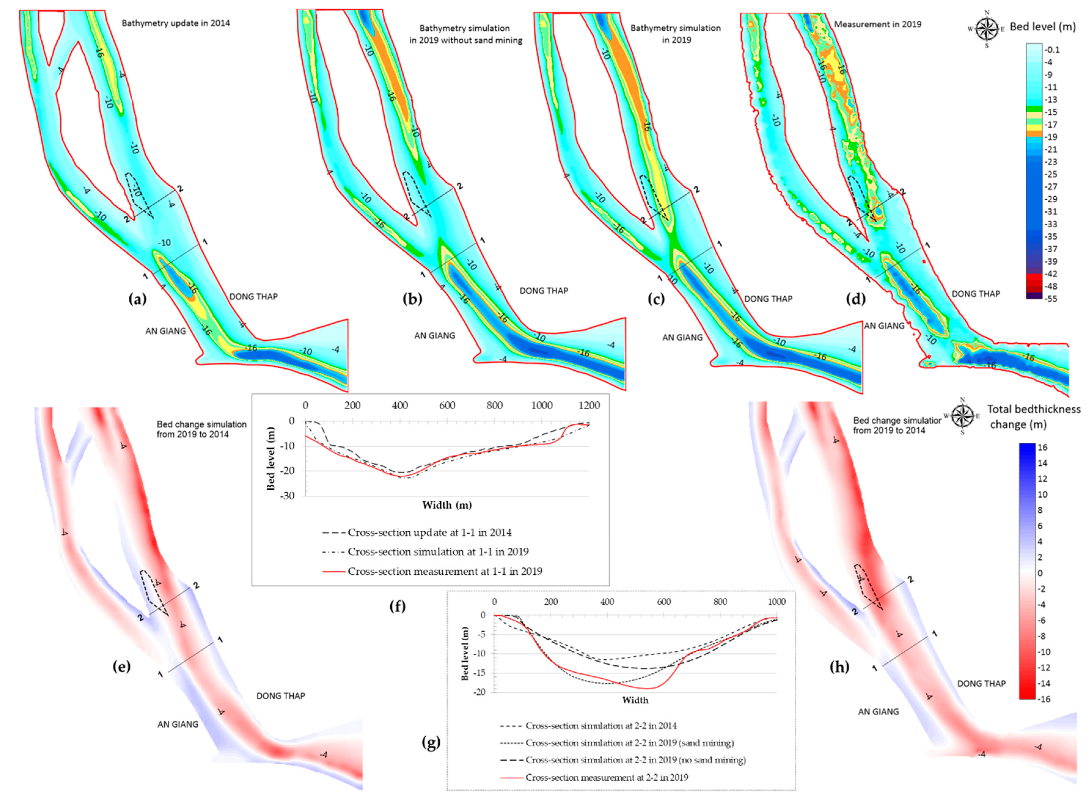
4.4.4. From 2014 to 2019 (SC4A and SC4B)

SC4A: During this period, alluvial sediment was reduced by two-thirds compared to the previous period [14], and, accordingly, the sediment boundary was also reduced. The calculation results show that the whole study area tended to erode, even at the site of Tan An mine (which has stopped operating), which gradually eroded (see Figure 16f,h).
The results were compared between the observations and simulations at cross-section 2.2, which recorded a small error in 2019 (Figure 16g). The sand mining in this area made stream erosion flow towards Vinh Hoa sand mine and connected to the stream erosion downstream (Figure 16c,h).
At the cross-section 1.1, the riverbed eroded from a depth of −20 to about −22 m (the speed erosion of 0.4 m/year). Moreover, in the Vinh Hoa communes, An Giang Province, the Vinh Hoa sand mine was in operation (see Table 1). The calculation results show that there was an eroded channel here (the bed elevation changed from −12 (2014) to −18 m (2019)), with an erosion speed of 1.2 m/year. The bed change here caused the flow to change its path towards Dong Thap.
SC4B: If there were no sand mine, the erosion channel would not have expanded downstream and eroded in the middle of the river (Figure 16b,e). The bed level at Vinh Hoa sand mine, in this case, was slightly eroded, at about 0.2 m/year.
Thus, the operation of Tan An sand mine in the area (2002–2006) caused the channel to deviate slightly from An Giang and created a slight erosion channel in 2006 (−23 m). From 2006 through 2014, although Tan An mine was not in operation, the riverbed in this place recovered quite slowly with a small accretion rate (0.25 m/year). The operation of the Vinh Hoa sand mine has created a deep erosion channel here, and made the main flow move completely over Vinh Hoa sand mine during the period of 2014–2019. Moreover, a decrease in the amount of alluvium caused Tan An sand mine to erode again (the average rate of erosion was 0.4 m/year). Sand mining made the erosion channel move towards sand mines, with a faster erosion speed in the absence of sand mining. In the case in An Giang, the erosion canal moved closer to shore (the sand mining site was near the shore). The erosion channel near the riverbank causes the slope of the riverbank in An Giang to be steeper. As a result, the stability of the bank decreases; this is one of the causes of a river bank collapse. This matter directly affects the socio-economic development planning of the local area and construction along the river in An Giang Province.

5. Conclusions

The results of simulating the sedimentation progress of the study area using the model were appropriate, compared to the measurement bathymetry of specific years (2006, 2014, and 2019) when Tan An and Vinh Hoa sand mines were added. Due to the impact of sand mining, the main flow changed, producing a significant effect on the hydrodynamic regime, as well as the morphology of the riverbed in the study area. The analysis showed that sand mining made the erosion channel move towards the sand mines, after which the erosion speed increased when there was no sand mining.
The simulation period was quite long (1999–2019), making it sufficient to prove the good applicability of the model to other river areas where sand mines are operating. The study results will help policymakers in the Tien river area (An Giang, Dong Thap) in planning bank protection works, agricultural planning, and sand mining management.
In addition, harnessing the power of accelerators such as GPUs can help run the numerical simulations up to 23x times faster. This helps quickly verify the practical data collected coarsely and reduces the risk of critical situations, such as resident evacuations, when riverbank failure happens. In future work, we plan to extend our implementation to a distributed GPU system to study larger areas of rivers (or even oceans) using the numerical model.

Author Contributions

Conceptualization, T.T.K., N.T.B., W.-K.J., T.M.Q. and N.K.P.; Data curation, N.D.Q.H. and P.A.T.; Funding acquisition, N.K.P.; Methodology, T.T.K., T.M.Q., W.-K.J. and N.T.B.; Resources, N.D.Q.H. and P.A.T.; Software, T.T.K., N.T.M.H., P.A.T., S.H., T.M.Q., W.-K.J. and N.T.B.; Supervision, N.K.P., W.-K.J. and N.T.B.; Validation, T.T.K.; Visualization, N.T.M.H., S.H., and T.M.Q.; Writing—original draft, T.T.K., N.K.P., T.M.Q. and N.T.B.; Writing—review and editing, T.T.K., T.M.Q., N.T.B. All authors have read and agreed to the published version of the manuscript.

Funding

This research was funded by the Institute for Computational Science and Technology, with the topic “Development of bank erosion numerical model basing on HPC in connection with hydraulic model and to apply for some river reaches of the Mekong River”, (Grant No. NĐT.28.KR/17) and the National Research Foundation of Korea (NRF-2014K1A3A1A05034557).

Conflicts of Interest

The authors declare no conflict of interest.

Nomenclatures

uDepth-averaged horizontal velocity components in x-direction (m/s)
νDepth-averaged horizontal velocity components in y-direction (m/s)
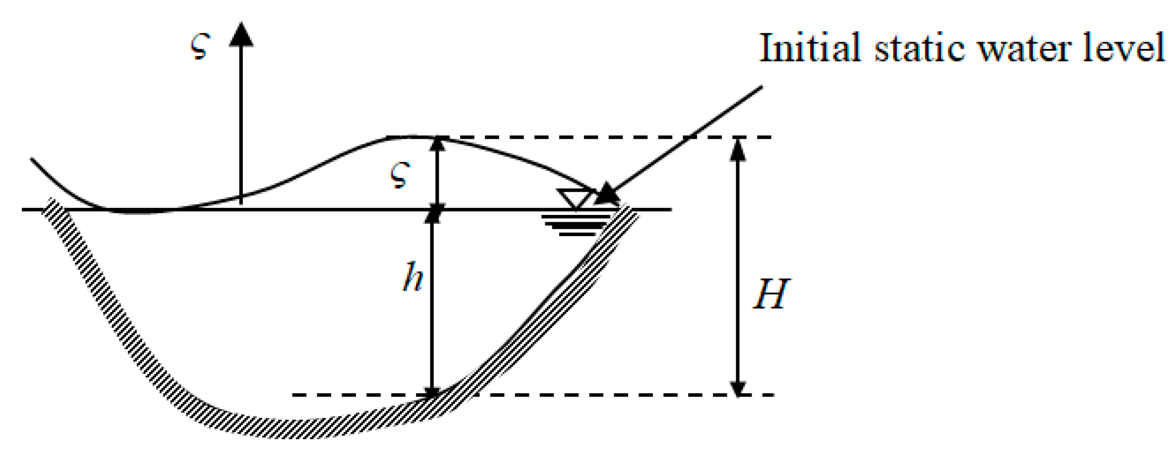
ςFluctuation of the water surface, compared to a “zero” level (m)
hStatic depth from the still water surface to the bed (m)
KFriction bed coefficient
AEddy horizontal viscosity coefficient (m2/s)
gAcceleration gravity (m/s2)
CDepth-averaged concentration of the suspended load (m3/m3)
KxDispersion coefficient in the Ox direction (m2/s)
KyDispersion coefficient in the Oy direction (m2/s)
HAverage depth used in the model (H=h+ ς) (m)
γvVelocity coefficient for the depth; calculated from γ v = ( 1 Z ) [ 1 ( a H ) 0.2 ] ( 1.2 Z ) [ 1 ( a H ) 1 Z ]
ZSuspension number defined after Van Rijn (1993), Z = ω s χ ( u * + 2 ω s )
χVon Karman constant = 0.4
uBed shear velocity, u * = g C h 2 ( u 2 + v 2 )
ChChezy coefficient, C h = 18 log ( 12 H K s )
KsBed roughness, Ks = 3D90
D90Diameter of particle that is equal to or less than 90% of the mass of the particles present
SStanding for erosion and deposition rates (m/s).
MSediment size-dependent coefficient after Van Rijn (1993): 0,00001 (kg/m2/s)
CbConcentration of bedload, (m3/m3)
ωsmParticle fall velocity in a mixture of water and sediment (m/s), ω s m = ( 1 C ) 4   ω s
ωsParticle fall velocity, ω s   = (   ρ s ρ   1 ) g d 2 18 v
DMean diameter of the particle (m)
νKinematic viscosity coefficient (m2/s)
τeCritical bed shear stress for erosion at the bottom (N/m2)
τdCritical bed shear stress for deposition at the bottom (N/m2)
τbBed shear stress (N/m2), τ b = 1 8 ρ f w V 2
fwFriction coefficient of Darcy – Weisbach, calculated from the Chezy formula; f w = 8 g n r 2 H 1 / 3
ρMass density of water, (kg/m3)
ρsDensity of particles, (kg/m3)
nrRoughness coefficient
εpVoid ratio of sediment
D*Dimensionless particle parameter D = d m [ g ( ρ s ρ 1 ) ν 2 ] 1 3
TDimensionless bed shear stress: T = [ u * 2 u * , c r 2 u * , c r 2 ]
u*,crCritical depth-averaged flow velocity based on Shields (m/s), u * , c r = 0.25 ( ρ s ρ 1 ) 8 15 d 9 15 g 8 15 ν 1 15
qbBedload q b = 0 . 0 5 3 ( ( ρ s ρ 1 ) g ) 0 . 5 d m 1 . 5 T 2 . 1 D 0 . 3 ( u , v ) u 2 + v 2
hiBottom depth at the calculation node (m)
ΔxThe distance between two nodes (m)
npPerpendicular to the shoreline

References

  1. Baena-Escudero, R.; Rinaldi, M.; García-Martínez, B.; Guerrero-Amador, I.C.; Nardi, L. Sediment mining in alluvial channels: Physical effects and management perspective. Geomorphology 2019, 337, 15–30. [Google Scholar] [CrossRef]
  2. Chen, D.; Acharya, K.; Stone, M. Sensitivity analysis of nonequilibrium adaptation parameters for modeling mining-pit migration. J. Hydraul. Eng. 2010, 136, 806–811. [Google Scholar] [CrossRef] [Green Version]
  3. Kim, C. Impact analysis of river aggregate mining on river environment. KSCE J. Civil Eng. 2005, 9, 45–48. [Google Scholar] [CrossRef]
  4. Kondolf, G.M. Hungry water: Effects of dams and gravel mining on river channels. Environ. Manag. 1997, 21, 533–551. [Google Scholar] [CrossRef]
  5. Martín-Vide, J.P.; Ferrer-Boix, C.; Ollero, A. Incision due to gravel mining: Modeling a case study from the Gallegoriver, Spain. Geomorphology 2010, 117, 261–271. [Google Scholar] [CrossRef]
  6. Bandita, B.; Arup, K.S.; Bimlesh, K. Mining pit migration of an alluvial channel: Experimental and numerical investigations. ISH J. Hydraul. Eng. 2020, 26, 448–456. [Google Scholar] [CrossRef]
  7. Bandita, B.; Bimlesh, K.; Arup, K.S. Dynamic characterization of the migration of a mining pit in an alluvial channel. Int. J. Sediment Res. 2019, 34, 155–165. [Google Scholar] [CrossRef]
  8. Yuill, B.T.; Gaweesh, A.; Allison, M.A.; Meselhe, E.A. Morphodynamic evolution of a lower Mississippi River channel bar after sand mining. Earth Surf. Process. Landf. 2016, 41, 526–542. [Google Scholar] [CrossRef]
  9. Jia, P.; Dong, C.; Brendan, T.Y. Modeling Evolution of a Large Mining Pit in the Lower Mississippi River. In Proceedings of the World Environmental and Water Resources Congress, Pittsburgh, Pennsylvania, 19–23 May 2019; pp. 287–295. [Google Scholar]
  10. Van Rijn, L.C. Sedimentation of dredged channels by currents and waves. J. Waterw. Port Coast. Ocean Eng. 1986, 112, 541–559. [Google Scholar] [CrossRef]
  11. Adamson, P.T.; Rutherfurd, I.D.; Peel, M.; Conlan, I.A. The hydrology of the Mekong River. In The Mekong; Elsevier: Amsterdam, The Netherlands, 2009; pp. 53–76. [Google Scholar]
  12. Gupta, A.; Liew, S.C. The Mekong from satellite imagery: A quick look at a large river. Geomorphology 2007, 85, 259–274. [Google Scholar] [CrossRef]
  13. Halls, A.S.; Conlan, I.; Wisesjindawat, W.; Phouthavongs, K.; Viravong, S.; Chan, S.; Vu, V.A. Atlas of Deep Pools in the Lower Mekong River and Some of its Tributaries; Mekong River Commission: Phnom Penh, Cambodia, 2013. [Google Scholar]
  14. Jordan, C.; Tiede, J.; Lojek, O.; Visscher, J.; Apel, H.; Nguyen, H.Q.; Schlurmann, T. Sand mining in the Mekong Delta revisited-current scales of local sediment deficits. Sci. Rep. 2019, 9, 17823. [Google Scholar] [CrossRef]
  15. Bravard, J.P.; Goichot, M.; Gaillot, S. Geography of sand and gravel mining in the Lower Mekong River. First survey and impact assessment. EchoGéo 2013, 26. [Google Scholar] [CrossRef] [Green Version]
  16. Hackney, C.; Darby, S.; Parsons, D.; Leyland, J.; Best, J.; Aalto, R.; Nicholas, A. Unsustainable in-channel sand mining threatens sand delivery to the Mekong delta. In Proceedings of the 20th EGU General Assembly, Vienna, Austria, 4–13 April 2018. [Google Scholar]
  17. Best, J.; Hackney, C.R.; Darby, S.E.; Parsons, D.R.; Leyland, J.; Aalto, R.E.; Nicholas, A.P.; Houseago, R.C. River bank instability induced by unsustainable sand mining in the Mekong River. In Proceedings of the AGU Fall Meeting 2019, San Francisco, CA, USA, 9–13 December 2019; American Geophysical Union: Washington, DC, USA, 2019. [Google Scholar]
  18. Hoai, H.C.; Bay, N.T.; Khoi, D.N.; Nga, T.N.Q. Analyzing the causes producing the rapidity of river bank erosion in Mekong Delta. Vietnam J. Hydro-Meteorol. 2019, 7, 42–50. (In Vietnamese) [Google Scholar]
  19. Filip, H. Studies of the morphological activity of rivers as illustrated by the River Fyris, Bulletin. Geol. Inst. Upsalsa 1935, 25, 221–527. [Google Scholar]
  20. Kondolf, G.M.; Schmitt, R.J.; Carling, P.; Darby, S.; Arias, M.; Bizzi, S.; Castelletti, A.; Cochrane, T.A.; Gibson, S.; Kummu, M.; et al. Changing sediment budget of the Mekong: Cumulative threats and management strategies for a large river basin. Sci. Total Environ. 2018, 625, 114–134. [Google Scholar] [CrossRef] [PubMed] [Green Version]
  21. Babu, K.; Dwarakish, G.; Jayakumar, S. Modeling of sediment transport along Mangalore coast using mike 21. In Proceedings of the International Conference on Coastal and Ocean Technology, Chennai, India, 10–12 December 2003. [Google Scholar]
  22. Daghigh, H.; Khaniki, A.K.; Bidokhti, A.A.; Habibi, M. Prediction of bed ripple geometry under controlled wave conditions: Wave-flume experiments and MIKE21 numerical simulations. Indian J. Geo-Mar. Sci. 2017, 46, 529–537. [Google Scholar]
  23. Jia, Y.; Wang, S.S. Numerical model for channel flow and morphological change studies. J. Hydraul. Eng. 1999, 125, 924–933. [Google Scholar] [CrossRef]
  24. Kopmann, R.; Merkel, U.H. Using reliability analysis in morphodynamic simulation with TELEMAC-2D/SISYPHE. In Proceedings of the XIXth TELEMAC-MASCARET User Conference, Oxford, UK, 18–19 October 2012. [Google Scholar]
  25. Villaret, C.; Hervouet, J.M.; Kopmann, R.; Merkel, U.; Davies, A.G. Morphodynamic modeling using the Telemac finite-element system. J. Comput. 2013, 53, 105–113. [Google Scholar] [CrossRef]
  26. Safarzadeh, A.; Neyshabouri, A.S.; Dehkordi, A. 2D Numerical Simulation of Fluvial Hydrodynamics and Bed Morphological Changes. In AIP Conference Proceedings; American Institute of Physics: College Park, MA, USA, 2009. [Google Scholar]
  27. Ahn, J.; Lyu, S. Analysis of flow and bed change on hydraulic structure using CCHE2D: Focusing on Changnyong-Haman. J. Korea Water Resour. Assoc. 2013, 46, 707–717. [Google Scholar] [CrossRef] [Green Version]
  28. Bay, N.T.; Khoi, D.N.; Kim, T.T.; Phung, N.K. Research on bottom morphology and Lithodynamic processes in the coastal area using the numerical Model: Case Studies of Can Gio and Cua Lap, Southern Vietnam. Vietnam J. Hydro-Meteorol. 2018, 2, 43–53. [Google Scholar]
  29. Bay, N.T.; Toan, T.T.; Phung, N.K.; Nguyen-Quang, T. Numerical investigation on the sediment transport trend of Can Gio Coastal Area (Southern Vietnam). J. Mar. Environ. Eng. 2012, 9, 191–211. [Google Scholar]
  30. Guan, M.; Liang, Q. A two-dimensional hydro-morphological model for river hydraulics and morphology with vegetation. Environ. Model. Softw. 2017, 88, 10–21. [Google Scholar] [CrossRef] [Green Version]
  31. Ikeda, S. Sediment transport and sorting at bends. River Meand. 1989, 12, 103–125. [Google Scholar]
  32. Van Rijn, L.C. Sediment Transport, Part II: Suspended Load Transport. J. Hydraul. Eng. 1984, 110, 1613–1641. [Google Scholar] [CrossRef]
  33. Wu, W. Depth-averaged two-dimensional numerical modeling of unsteady flow and nonuniform sediment transport in open channels. J. Hydraul. Eng. 2004, 130, 1013–1024. [Google Scholar] [CrossRef]
  34. Wu, W.; Shields, F.D., Jr.; Bennett, S.J.; Wang, S.S. A depth-averaged two-dimensional model for flow, sediment transport, and bed topography in curved channels with riparian vegetation. Water Resour. Res. 2005, 41. [Google Scholar] [CrossRef]
  35. Bay, N.T.; Kim, T.T.; Hoai, H.C.; Tai, P.A.; Huy, N.D.Q.; Phung, N.K. HYDIST model and the approach of solving sediment concentration at open boundaries. Vietnam J. Hydro-Meteorol. 2019, 704, 57–64. (In Vietnamese) [Google Scholar] [CrossRef]
  36. Mattamana, B.A.; Varghese, S.; Paul, K. River Sand Inflow Assessment and Optimal Sand Mining Policy Development. Int. J. Emerg. Technol. Adv. Eng. 2013, 3, 305–317. [Google Scholar]
  37. Yao, J.; Zhang, D.; Li, Y.; Zhang, Q.; Gao, J. Quantifying the hydrodynamic impacts of cumulative sand mining on a large river-connected floodplain lake: Poyang Lake. J. Hydrol. 2019, 579, 124156. [Google Scholar] [CrossRef]
  38. Obot, O.I.; Ekpo, I.F.; David, G.S. The Effect of Sand Mining on the Physico-Chemical Parameters of Ikot Ekpan River, Akwa Ibom State, Nigeria. J. Aquat. Sci. Mar. Biol. 2019, 2, 21–24. [Google Scholar]
  39. Okorie, P.U.; Acholonu, A.D.W. Effect of Commercial Sand Mining on Water Quality Parameters of Nworie River in Owerri, Nigeria. Proc. Niger. Acad. Sci. 2018, 11, 1–8. [Google Scholar]
  40. Cui, M. Compact alternating direction implicit method for two-dimensional time fractional diffusion equation. J. Comput. Phys. 2012, 231, 2621–2633. [Google Scholar] [CrossRef]
  41. Gong, C.; Bao, W.; Tang, G.; Jiang, Y.; Liu, J. Computational challenge of fractional differential equations and the potential solutions: A survey. Math. Probl. Eng. 2015, 2015, 258265. [Google Scholar] [CrossRef] [Green Version]
  42. Harris, M. Fast fluid dynamics simulation on the GPU. In ACM SIGGRAPH 2005 Courses on—SIGGRAPH ’05; Addison-Wesley Professional: Boston, MA, USA, 2005; Volume 220, pp. 637–666. [Google Scholar]
  43. Mei, X.; Decaudin, P.; Hu, B.-G. Fast hydraulic erosion simulation and visualization on GPU. In Proceedings of the 15th Pacific Conference on Computer Graphics and Applications (PG’07), Maui, HI, USA, 29 October–2 November 2007. [Google Scholar]
  44. Guidolin, M.; Kapelan, Z.; Savic, D.; Giustolisi, O. High performance hydraulic simulations with epanet on graphics processing units. In Proceedings of the 9th International Conference on Hydroinformatics, Tianjin, China, 7–11 September 2010. [Google Scholar]
  45. Wu, Z.Y.; Eftekharian, A.A. Parallel artificial neural network using CUDA-Enabled GPU for extracting hydraulic domain knowledge of large water distribution systems. In Proceedings of the World Environmental and Water Resources Congress, Palm Springs, CA, USA, 22–26 May 2011; pp. 79–92. [Google Scholar] [CrossRef]
  46. Dorsey, J.; Edelman, A.; Jensen, H.W.; Legakis, J.; Pedersen, H.K. Modeling and rendering of weathered stone. In Proceedings of the 26th Annual Conference on Computer Graphics and Interactive Techniques, Los Angeles, CA, USA, 8–13 August 1999. [Google Scholar]
  47. Liu, Y.Q.; Zhu, H.B.; Liu, X.H.; Wu, E.H. Real-time simulation of physically based on-surface flow. Vis. Comput. 2005, 21, 727–734. [Google Scholar] [CrossRef]
  48. Gupta, A. Chapter 3—Geology and landforms of the Mekong basin. In The Mekong. Aquatic Ecology; Campbell, I.C., Ed.; Academic Press: Cambridge, MA, USA, 2009; pp. 29–51. [Google Scholar]
  49. Hai, H.Q. Correlation of erosion—Aggradation in areas along Tien and Hau Rivers. Vietnam J. Earth Sci. 2011, 33, 37–44. (In Vietnamese) [Google Scholar] [CrossRef] [Green Version]
  50. Kuenzer, C.; Guo, H.; Huth, J.; Leinenkugel, P.; Li, X.; Dech, S. Flood mapping and flood dynamics of the Mekong Delta: ENVISAT-ASAR-WSM based time series analyses. Remote Sens. 2013, 5, 687–715. [Google Scholar] [CrossRef] [Green Version]
  51. Van Rijn, L.C. Principles of Sediment Transport in Rivers, Estuaries and Coastal Seas; Aqua Publications: Amsterdam, The Netherlands, 1993; Volume 1006. [Google Scholar]
  52. Douglas, J. On the Numerical Integration of ∂^2u∂x^2+∂^2u∂y^2=∂u∂t by Implicit Methods. J. Soc. Ind. Appl. Math. 1955, 3, 42–65. [Google Scholar]
  53. Thomas, L. Elliptic Problems in Linear Differential Equations Over a Network: Watson Scientific Computing Laboratory; Columbia University: New York, NY, USA, 1949. [Google Scholar]
  54. Valero-Lara, P.; Martínez-Pérez, I.; Sirvent, R.; Martorell, X.; Peña, A.J. cuThomasBatch and cuThomasVBatch, CUDA Routines to compute batch of tridiagonal systems on NVIDIA GPUs. Concurr. Comput. Pract. Exp. 2018, 30, e4909. [Google Scholar] [CrossRef]
  55. The 2-Clause BSD License. Available online: http://www.opensource.org/licenses/bsd-license.php (accessed on 20 July 2019).
  56. National Center for Computational Hydroscience and Engineering (CCHE). CCHE2D: Two-Dimensional Hydrodynamic and Sediment Transport Model for Unsteady Open Channel Flows Over Loose Bed; Technical Report No. NCCHE-TR-2001-1; National Center for Computational Hydroscience and Engineering (CCHE): University, MS, USA, 2001. [Google Scholar]
  57. Nash, J.E.; Sutcliffe, J.V. River flow forecasting through conceptual models part I—A discussion of principles. J. Hydrol. 1970, 10, 282–290. [Google Scholar] [CrossRef]
  58. Moriasi, D.N.; Arnold, J.G.; Van Liew, M.W.; Bingner, R.L.; Harmel, R.D.; Veith, T.L. Model evaluation guidelines for systematic quantification of accuracy in watershed simulations. Trans. ASABE 2007, 50, 885–900. [Google Scholar] [CrossRef]
  59. Moriasi, D.N.; Gitau, M.W.; Pai, N.; Daggupati, P. Hydrologic and water quality models: Performance measures and evaluation criteria. Trans. ASABE 2015, 58, 1763–1785. [Google Scholar] [CrossRef] [Green Version]
  60. Mehta, A.J.; Hayter, E.J.; Parker, W.R.; Krone, R.B.; Teeter, A.M. Cohesive sediment transport. I: Process description. J. Hydraul. Eng. 1989, 115, 1076–1093. [Google Scholar] [CrossRef]
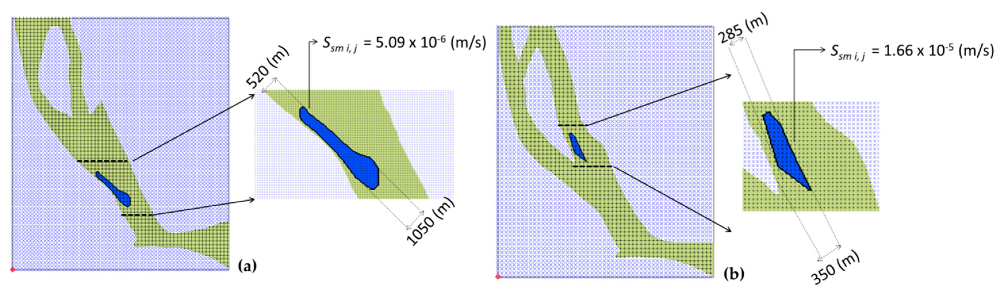
Figure 1. The study area (Source: Tan Chau bathymetry (a) collected on October 1999 from the Department of Investment and Construction Project of Tan Chau town area, An Giang, Vietnam; Tan Chau bathymetry (b) collected on October 2014 from The Southern Institute Of Water Resources Research; Mekong delta map (c) is referenced from Kuenzer et al. [50].
Water 12 02912 g001
Figure 2. Illustration of the initial static level.
Water 12 02912 g002
Figure 3. Tan An (a) and Vinh Hoa (b) sand mines position at Tien River.
Water 12 02912 g003
Figure 4. Input discharge Q(t) in 1999 (a) and 2018 (b); input water level ς(t) in 1999 (c) and 2018 (d); and the input total suspended solids (TSS) C(t) in 1999 (e) and 2018 (f).
Water 12 02912 g004
Figure 5. Calibration results at Tan Chau station from 11 July 2002 to 30 October 2002 for water level ς (m) (a) and discharge Q (m3/s) (b).
Water 12 02912 g005
Figure 6. Roughness coefficient for the study area.
Water 12 02912 g006
Figure 7. Observations and simulations at Tan Chau station from 10:00 6 June 2018 to 10:00 13 June 2018 for the water level ς (m) (a) and discharge Q (m3/s) (b).
Water 12 02912 g007
Figure 8. Observations and simulations at Tan Chau station for calibration TSS (g/l) (a) and validation TSS (g/l) (b).
Water 12 02912 g008
Figure 9. A visual comparison of the vector fields on the CPU (rendered using Surfer) (a) and on the graphics processing units (GPU) (rendered using Python) (b) after 15 h of simulation using 20 m-grid data.
Water 12 02912 g009
Figure 10. A visual comparison of the vector fields on the CPU (rendered using Surfer) (a) and on the GPU (rendered using Python) (b) after 15 h of simulation using 10 m-grid data.
Water 12 02912 g010
Figure 11. Scalability on 20 m-grid (a) and 10 m-grid (b); running time of 15 h.
Water 12 02912 g011
Figure 12. The initial bathymetry of the study area (a) and the velocity field of the peaking flood at 21:00 on 29 September 2002 (b).
Water 12 02912 g012
Figure 13. Simulation of the bed changes over 3 years from 1999 to 2002: (a,b) figures describing the results of simulations for 1999 and 2002, respectively; (c) the bed change simulation during the period; and (d) the comparison graphs of simulations at cross-section 1.1.
Water 12 02912 g013
Figure 14. Simulation of the bed changes over 4 years from 2002 to 2006: (a,c) the results of simulations for 2002 and 2006, respectively; (b) the case with no sand simulation for 2006; (d) riverbed measurements in 2006; (e,g) bed change simulations during the period with sand mining and no sand mining, respectively; (f) comparison graphs of simulations and measurements at cross-section 1.1.
Water 12 02912 g014
Figure 15. Simulation of the bed changes over the period of 8 years from 2006 to 2014: (a,b) results of the simulations for 2006 and 2014, respectively; (c) riverbed measurements for 2014; (d) bed change simulations during the period; (e) a comparison graph of simulations and measurements at cross-section 1.1.
Water 12 02912 g015
Figure 16. Simulation of the bed changes over 5 years from 2014 to 2019: (a,c) results of the simulations in 2014 and 2019, respectively; (b) the case of no sand simulations in 2019; (d) riverbed measurements in 2019; (e,h) bed change simulations during the period with no sand mining and sand mining, respectively; (f,g) comparison graphs of simulations and measurements at cross-sections 1.1 and 2.2, respectively.
Water 12 02912 g016
Table 1. Average exploitation speed of Tan An and Vinh Hoa sand mines.
Sand MineAnnual Output
(m3/year)
Square
(m2)
Average Exploitation Rate (m/s)-Ssm(i, j)
1999–20012002–20062007–20142014–2019
SC1SC2ASC2BSC3SC4ASC 4B
Tan An200,000910,00005.09 × 10-60000
Vinh Hoa200,000279,00000001.66 × 10-50
Table 2. Model parameters.
ParameterValue
Time step (Δt)2 s
Mean diameter of particle (D)0.01 mm
Diameter of particle 90% of the mass of particles present (D90)0.04 mm
Density of particles (ρs)2600 kg/m3
Kinematic viscosity coefficient (ν) 1.01 × 10 6 m2/s
Critical shear stress for deposition (τd)0.35 N/m2
Critical shear stress for erosion (τe)0.04 N/m2
Table 3. A direct comparison of running times on the CPU (a) and GPU (b) for 20 m- and 10 m-grid simulations.
20-m Grid10 m-Grid
Hours of SimulationRunning Time on the CPU (s)Running Time on the GPU (s)Accelerating FactorRunning Time on the CPU (s)Running Time on the GPU (s)Accelerating Factor
172.00612409.001626
2141.001211.75806.003225
3213.001911.210526321,196.004924
4282.002511.281,568.006624
5353.003111.387096771,953.008224
6425.003811.184210532,340.009924
7496.004411.272727272,724.0011623
8567.005011.343,110.0013224
9638.005711.192982463,494.0014824
10709.006311.253968253,852.0016523
11780.006911.304347834,198.0018123
12851.007611.197368424,572.0019823
13922.008211.243902444,946.0021523
14995.008911.179775285,323.0023223
151,068.009511.242105265,697.0024823
.....................
Publisher’s Note: MDPI stays neutral with regard to jurisdictional claims in published maps and institutional affiliations.

