Article

A Stochastic Model to Predict Flow, Nutrient and Temperature Changes in a Sewer under Water Conservation Scenarios

1
Water Innovation & Research Centre, Department of Chemical Engineering, University of Bath, Claverton Down, Bath BA2 7AY, UK
2
Department of Water Management, Faculty of Civil Engineering and Geosciences, Delft University of Technology, P.O. Box 5, 2600 AA Delft, The Netherlands
3
Amsterdam Institute for Advanced Metropolitan Solutions, Kattenburgerstraat 5, 1018 JA Amsterdam, The Netherlands
4
Waternet, P.O. Box 94370, 1090 GJ Amsterdam, The Netherlands
5
College of Engineering, Mathematics & Physical Sciences, University of Exeter, Harrison Building, North Park Road, Exeter EX4 4QF, UK
6
KWR Water Research Institute, P.O. Box 1072, 3430 BB Nieuwegein, The Netherlands
*
Author to whom correspondence should be addressed.
Water 2020, 12(4), 1187; https://doi.org/10.3390/w12041187
Submission received: 24 March 2020 / Revised: 10 April 2020 / Accepted: 15 April 2020 / Published: 21 April 2020
(This article belongs to the Special Issue Advances in Modeling and Management of Urban Water Networks)

Abstract

:
Reducing water use could impact existing sewer systems but this is not currently well understood. This work describes a new flow and wastewater quality model developed to investigate this impact. SIMDEUM WW® was used to generate stochastic appliance-specific discharge profiles for wastewater flow and concentration, which were fed into InfoWorks® ICM to quantify the impacts within the sewer network. The model was validated using measured field data from a sewer system in Amsterdam serving 418 households. Wastewater concentrations of total suspended solids (TSS), chemical oxygen demand (COD), total Kjeldahl nitrogen (TKN) and total phosphorus (TPH) were sampled on an hourly basis, for one week. The results obtained showed that the InfoWorks® model predicted the mass flow of pollutants well (R-values 0.69, 0.72 and 0.75 for COD, TKN and TPH respectively) but, due to the current lack of a time-varying solids transport model within InfoWorks®, the prediction for wastewater concentration parameters was less reliable. Still, the model was deemed capable of analysing the effects of three water conservation strategies (greywater reuse, rainwater harvesting and water-saving appliances) on flow, nutrient concentrations, and temperature in sewer networks. Results show through a 62% reduction in sewer flow, COD, TKN and TPH concentrations increased by up to 111%, 84% and 75% respectively, offering more favourable conditions for nutrient recovery.

Graphical Abstract

1. Introduction

Contemporary water cycle infrastructure has typically been developed to promote public health and safety by supplying wholesome drinking water and by transporting wastewater and stormwater out of urban areas as quickly as possible. This has led to linear water use (take, use, throwaway) that is sub-optimal on grounds of sustainability. With growing environmental awareness, the idea of a circular economy has emerged, and a paradigm shift is required to close the water cycle and re-classify wastes as resources to recover and reuse. Resource recovery from wastewater is more effective at high concentrations. This can be achieved through dewatering processes at treatment plants [1,2,3] but another option is to limit wastewater dilution in the collection process [4]. Limiting wastewater dilution can be achieved by reducing domestic drinking water use, separation of storm/wastewater systems and preventing groundwater inflow by repairing/replacing broken pipes. This reduces nutrient loss from the cycle whilst reduced drinking water demand and wastewater transportation volume could save cost by reducing demands on existing infrastructure. Transporting more concentrated flow with a smaller pipe/equipment size requirement is also facilitated. Urban water cycles could enable resource recovery if considered from this new value proposition. This philosophy has prompted the development of a water cycle model to investigate the effects of future water use behaviours on the urban water system, and ultimately highlight how these systems could deliver enhanced resource recovery. This paper describes the development of a stochastic wastewater quality model and the comparison of this model to monitored field data. The sewer model forms part of a wider aim to develop an integrated water cycle model using a combination of SIMDEUM® and InfoWorks® WS/ICM packages. The integrated model will predict flow and wastewater quality changes in both drinking water and wastewater infrastructures, to evaluate the consequences of future water use scenarios.
Water demand and water quality models can be developed as deterministic or stochastic models. In a deterministic model, the results are fully based on pre-set parameter values and initial conditions. Stochastic models will include randomness and each time the model is used it will produce a different output. The advantage of deterministic models is the relative ease of use, whilst stochastic models will provide better insight in the system’s dynamics. Because water use at the household level is extremely dynamic and follows random patterns, we have chosen to use a stochastic approach for this project as it gives a better reflection of reality.
A number of models have been developed to predict the impacts of various water conservation measures on the sewer system. These models have been largely deterministic [5,6,7] and have tested specific impacts of rainwater harvesting (RWH) and greywater reuse (GWR) on wastewater quality. Penn et al. [7] reported pollutant concentration increases of 6–42% COD, 7–73% TSS, 9–57% NH4-N and 7–52% PO4-P for flow decreases of 8–41%. However, these deterministic approaches model domestic wastewater production as a continuous discharge based on averaged data, assuming an identical water use pattern for all residents. In reality, individual household wastewater profiles are a discontinuous series of discrete points, and hence a stochastic model is needed to model household discharges which are more representative of this reality. Penn, et al. [8] published a stochastic wastewater generator that does not require a great amount of input data, but which is based on empirical sampling, and assumes that the observed flow data (from 15 households) represents the flow of the target population. The flow generator was used as an input to a network model that assessed ability of flow to move gross solids (GS) in the sewer. GS movement was assessed through calculating critical flow required to move solids, but this does not link solids/pollutant generation to the discharges themselves. If we are to model water use changes that have not yet been observed, a model based on deterministic methods or empirical sampling is insufficient. There is therefore need for a stochastic sewer model that is independent of observed data for predicting impacts of changing water use. To our knowledge there is currently no sewer model that links unique appliance-discharge patterns to the specific water quality attributes produced by household appliances. Developing a model with this capability will offer a better understanding of how and when pollutants/nutrients build up in sewers, and how various water use changes could affect this in future.
This paper utilises a more complex stochastic generator than that developed by Penn et al. [8]. This tool, SIMDEUM® [9], generates appliance-specific flow patterns based on probability parameters linked to appliance usage, household composition, and consumer water use behaviour [10]. Patterns produced by SIMDEUM® are specific to each appliance (e.g., toilet, sink and washing machine) which makes it possible to investigate explicit water use changes without assuming typical water usage patterns based on historical data. SIMDEUM WW® extends from SIMDEUM® to convert demand patterns into wastewater discharges, including thermal and nutrient loads [11]. This conversion is achieved through correcting the flow rate or delaying the time of discharge, e.g., toilets can take minutes to fill but seconds to discharge. Thermal and nutrient loads from each appliance are incorporated into the discharge profile by assigning typical (per use) load to each appliance.
Bailey et al. [12] developed a stochastic flow model to assess the impact of water conservation on the sewer. This model utilised stochastic household discharge patterns (generated with SIMDEUM WW®) as input to a sewer network model based in InfoWorks® ICM. The flow model was validated using data from an English catchment, provided by Wessex Water (UK-based water utility). The flow model was extended to include wastewater pollutant concentrations by linking typical wastewater quality data to appliance-specific discharges within SIMDEUM WW® and utilising the InfoWorks® ICM wastewater quality model [13]. The flow/quality model was used to simulate and compare a series of future water use scenarios. The wastewater quality aspect of this model, however, has not previously been compared to field data to assess its validity. This paper details a wastewater quality monitoring campaign conducted in a small housing estate in Amsterdam with that objective.
The paper is organised as follows: firstly, we describe the model development and the methodology behind the wastewater quality monitoring campaign. Followed by the framing of six future water use scenarios that were tested using the model. Then, a description of the Amsterdam-based catchment used to analyse the model precedes the model predictions and a comparison of modelled parameters with the measured data. Finally, we make key conclusions.

2. Methodology

A model was developed to simulate the effects of future water use scenarios in sewers. The Infoworks® ICM (Sewer Edition; Innovyze Ltd., Oxfordshire, UK) hydraulic and wastewater quality model was used to simulate the sewage system. This model was integrated with stochastic discharge patterns generated using SIMDEUM® and SIMDEUM WW® [10,14]. The MATLAB® codes behind SIMDEUM® were edited to make its outputs compatible with InfoWorks® ICM. Six future water use scenarios were framed and simulated using the validated model, allowing flow and concentration effects to be evaluated.
Infoworks® ICM Sewer Edition is an industry standard for 1-dimensional sewer network modelling. The software offers accurate analysis of hydraulics and water quality in sewer and stormwater networks. The model uses a network of nodes and conduits and solves the flow and mass balances for the network, based on water quantity and quality input, fed into the model via the nodes. The geometry of the network and the shape of the conduits is defined by geographical input and data from the real network.

2.1. Household Discharge Modelling

2.1.1. Hydraulic Discharge Model

The SIMDEUM® software tool was developed in the Netherlands for accurate water demand modelling. It can generate household water demand patterns based on statistical and probabilistic information about inhabitants and their appliance usage [10]. The SIMDEUM® pattern generator was calibrated for use in the studied catchment (Prinseneiland), which is described in Section 2.4.1, details of the studied catchment are shown in Section 3.

2.1.2. Wastewater Quality Loading

SIMDEUM WW® was used to link each wastewater discharge with an appliance-specific wastewater quality profile. SIMDEUM WW® originally included very little detail on pollutant discharges, having been used simply to demonstrate the possibility of nutrient discharge modelling [11,15]. Therefore, a review of relevant literature [5,15,16,17,18,19] was conducted to find appropriate input values for nutrient simulation. These input parameters describe pollutant mass per discharge for each household appliance (see Table 1), and the derivation of these parameters is described in Bailey et al. [13]. The nutrient discharge aspect of SIMDEUM WW® has never been validated. Through comparison of the wastewater quality model with measured data from this work, the phosphorus (TPH) parameters reported in literature were found to be too high. This is due to recent changes in EU legislation reducing phosphorus use in detergents [20]. The phosphorus parameters were corrected to align with this legislation and are highlighted in bold in Table 1. The phosphorus associated with the kitchen tap was approximated as in Comber et al. [21] where it was found to be 0.03 g person-1 day-1. It was assumed that this much phosphorus enters the sewer through the disposal of food scraps. The other value shown in Table 1, i.e., 0.03 g use-1, which depicts quality profile for each discharge, was found by calibration based on observed wastewater data and above assumed phosphorus value. The phosphorus from toilet use was updated in accordance with Comber et al. [21], and assuming, on average, six toilet uses per person, per day.
Quality of non-potable water sources was quantified using data from Penn et al. [6] (greywater) also Ward et al. [22] and Farreny et al. [23] (rainwater)—see Supplementary Information. This was combined with appliance pollutant quantities, shown in Table 1.

2.2. Stochastic Sewer Model

Wastewater flow and quality were simulated through a sewer network using InfoWorks® ICM (Sewer Edition; Innovyze Ltd., Oxfordshire, UK). Stochastic household discharge patterns, described in Section 2.1, were imported into InfoWorks® ICM to produce time-varying domestic wastewater event. Each property has a unique flow and associated wastewater concentration profile as input to the sewer; discharges were input with one-minute intervals.
InfoWorks® ICM incorporates both hydraulic and wastewater quality modelling components. The hydraulic component was validated by Bailey et al. [12] using measured flow, depth and velocity data. Saint-Venant equations govern hydraulics in InfoWorks® ICM. The wastewater quality model runs parallel to the hydraulic model, as described in Bailey et al. [13], but was not validated. The concentration of dissolved pollutants and suspended sediment at every node in the sewer network is calculated for every time step using the InfoWorks® Network Model. The governing equation at a node is given by conservation of mass, Equation (1). Pollutant inflows arrive from incoming conduits and any external sources, in this case, wastewater events (household discharges). It is assumed that nodes are well-mixed and there is no deposition or accumulation.
d M J d t = i Q i c i + d M s J d t o Q o c o
where:
M J = mass of suspended sediment or dissolved pollutant in node J (kg)
Q i = flow into node J from link i (m3 s−1)
c i = concentration in the flow into node J from link i (kg m−3)
M s J = additional mass entering node J from external sources (kg)
Q o = flow from node J to link o (m3 s−1)
c o = concentration in the flow from node J to link o (kg m−3)
The InfoWorks® Conduit Model then calculates the concentration of dissolved pollutants and suspended sediment in each conduit. A conduit is a conceptual link of defined length between two nodes. One-dimensional flow is assumed in the conduit, as are well-mixed concentrations across each section of the conduit. Pollutants are assumed move through the conduit with the local mean flow velocity, and dispersion along the conduit is negligible. Wastewater determinants were all treated as dissolved pollutants because InfoWorks® ICM software fails to recognise time-varying suspended solid input. The authors have been advised that this shortfall will be corrected in a future software update. Therefore, wastewater determinants in the model are transported through advection, with no erosion, deposition, or accumulation of sediments. The advective mass flow between each element is shown in Equation (2).
F a = F m × c u p w i n d
where:
F a = mass flow through the face due to advection (kg s−1)
F m = volumetric flow through the face (m3 s−1)
c u p w i n d = c l if volumetric flow goes from left to right element, c r otherwise (kg m−3); c l , c r = determinant concentration in respectively the left and right element
Adjusting to Allow for Mixing in the Sampling Tank
The sampling campaign, described in Section 2.3.2, generated data on wastewater in the pump feed tank rather than wastewater flowing in the sewer system (see Figure 1). As the sewage flows into the tank it mixes with the held-up water and thus the samples will reflect a dampened wastewater concentration compared to model predictions. The sewer model output was adjusted to allow for this mixing to allow comparison of model predictions with sampled concentration data. Equation (3) is the derived expression for concentration in the tank ( C A ), assuming the volume remains approximately constant (average volume of 1.6 m3, midway between high and low levels). It also assumes that no reactions occur in the tank and the wastewater has a constant density.
C A t = C A , i n t C A , o 1 e Q t V t
where:
C A = Concentration of pollutant A in the tank (kg m−3)
C A ,   i n = Concentration of pollutant A into the tank (kg m−3)
C A , o = Initial concentration of pollutant A (kg m−3)
Q = Flowrate into tank (m3 s−1)
V = Tank volume (m3)
t = Time (s)

2.3. Methodology for Field Testing

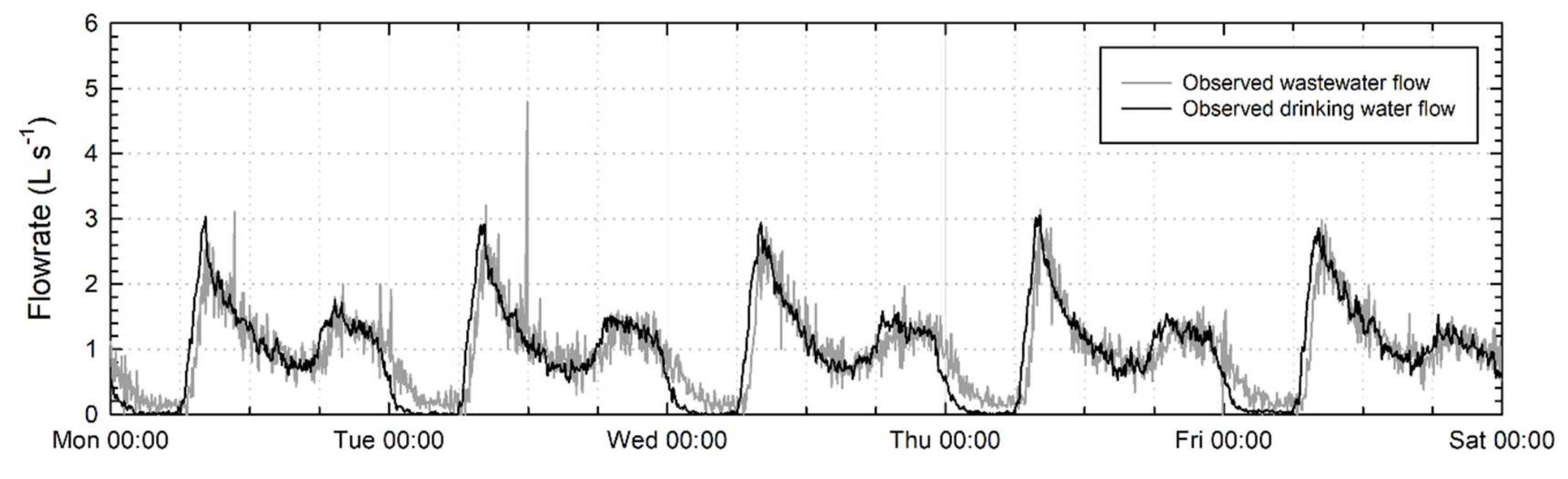
2.3.1. Data Availability for Validating the Hydraulic Discharge Model

The Prinseneiland catchment (See Section 3.1) has three sources of hydraulic water network data. Two water mains supply drinking water to the island; a flow meter was present in each, providing live data recording of water demand. Fifty-eight percent of catchment households have a water meter recording specific water use, but this is mainly for billing purposes as data is summed over the period between physical meter readings. The final data source was provided by pump flow and tank level readings, recorded at the wastewater pumping station. Readings are recorded every 2–5 min dependant on changes recorded by the level controller. A pump switches on when the tank level reaches the programmed high level (above the inlet pipe) and off when the level reaches the programmed low level (above the pump). The volumetric flowrate through the pump was measured using an ECOFLUX electromagnetic flowmeter (www.krohne.com) (accuracy ± 0.5% of the measured value at velocities ≥ 0.4 m s−1 and ± 0.002 m s−1 if velocity is below 0.4 m s−1). The tank level was measured using two VEGABAR 52 (www.vega.com) sensors, where the deviation is reported to be less than 0.075%. By performing a mass balance on the flow through the pump and the changing level in the tank (Equation (4)), it was possible to convert these readings into a sewer flow profile (Equation (5)).
V τ n , τ n + 1 = P C n τ n + 1 τ n + A L S n + 1 L S n S 1 + A L S n + 1 L S n S 2 2
Q t = t n = 0 V τ n , τ n + 1 t
where:
V τ n ,   τ n + 1 = Volume entering the tank between level sensor readings (m3)
P C = Pumping capacity (m3 s−1)
L S = Tank level (m)
A = Tank area (m2)
S 1 , S 2 = Level sensors
τ = Sample time (s)
Q t = Wastewater flowrate into the tank (m3 s−1)
t = Time (s)
At the end of August 2019, a wastewater quality campaign was carried out on Prinseneiland to collect data necessary for validating the wastewater quality component of the stochastic sewer model. The campaign was conducted continuously over 7 days, under dry weather conditions. Wastewater was sampled from the pump wet well at the end of the catchment. All Water Services (www.aws-water.nl) carried out the fieldwork and the wastewater samples were analysed by Eurofins Omegam. A vacuum sampling device was used (photographs in the Supplementary Information). The sampling cabinet was placed within a portable toilet at street level to comply with space constraints and protect apparatus from damage. The sampling hose was secured at the sewer inlet to the wet well in such a way that the end of the hose was approximately 3 cm below the cut-off level of the pump. This ensured that the wastewater was as “fresh” as possible when sampled from the tank, and thus most representative of the sewer flow. This method meant it was always possible to draw samples from the chamber, but during the night where wastewater flow is low, there is the possibility that stagnant wastewater is sampled. The sampling cabinet contained 24 1 L bottles into which a 50 mL sub-sample was drawn every 3 min, i.e., 20 sub-samples per hour make up the 1 L sample for that hour. The sample collection vessels were held at 1–5 °C. Sampling was carried out according to Dutch standard ‘NEN 6600-1 (NL) Water—Sampling—Part 1: Waste water from March 2009. Every 24 h the completed samples were removed from the cabinet and decanted into three separate packages for separate analysis (see Table 2), and nitrogen and phosphorus were analysed from the same package. Samples were preserved on site according to Dutch standard ‘NEN-EN-ISO 5667-3 (s) Water—Sampling—Part 3: Conservation and treatment of water samples’ and were delivered daily to the analysis laboratory under cooling.

2.3.2. Quality of Sampling and Analysis Work

AWS are accredited according to the requirements as laid down in NEN-EN-ISO/IEC 17025: 2005 and Dutch Accreditation Council (RvA) regulations under number L599. Eurofins Omegam laboratory in Amsterdam (who carried out the sample analysis) is also accredited by RvA.

2.3.3. Wastewater Quality Parameters

The parameters analysed and the procedures followed by the laboratory are shown in Table 2.

2.4. Model Validation

2.4.1. Procedure for Model Calibration

The SIMDEUM® model was calibrated by adjusting input variables describing household occupancy, home–presence, and specific details of household water use in the area. Households are characterised as either a single, dual, or family occupancy. Average occupancy and family size are also defined. The household data was derived from census data from the local government of the study area. Home presence data is culture and area-specific, and details typical times that people rise, go to work and go to bed. These data were obtained from the Netherlands Institute for Social Research (SCP) that conducts a five-year time-budget survey. Comparison of the model output with monitored catchment data showed a local deviation from the national survey data on wake-up time, so this was adjusted on a case-specific basis. Household water use data is available from local water companies and should be input to the model to describe typical water use for each household appliance. The specific model adaptions made for the studied catchment are detailed in Section 3.2.

2.4.2. Procedure for Model Validation

Validation of the model was conducted by assessing the model performance over an average week. Dry weather flow data was selected at various points of the year (2 weeks from each season) to produce an average water use pattern of the catchment in order to compare with the model. The goodness of fit of model output was evaluated by computation of the Nash–Sutcliffe efficiency ( N S E ) and the root mean squared error ( R M S E ). The similarity of the flow patterns was evaluated with the correlation coefficient ( R ). The equations for N S E , R M S E and R are found below in Equations (6–8).
N S E = 1 i = 1 n x o b s x s i m 2 i = 1 n x o b s x ¯ 2
R M S E = 1 n 1 i = 1 n x o b s x s i m 2
  R   X ,   Y = x x ¯ y y ¯ x x ¯ 2 y y ¯ 2
where:
x o b s = Observed parameter
x s i m = Simulated parameter
x ¯ , y ¯ = Sample mean of parameters x , y

2.5. Impact Assessment for Water Conservation Technologies

The development and validation of the sewer model allow it to be used to predict the effect of future scenarios. Table 3 describes the future scenarios that were developed for testing in the Prinseneiland catchment. These scenarios were based on total area reform (100% implementation). Water use scenarios include “Eco”, which involves an upgrade of household appliances (such as 1 L flush toilets and water-saving showers) and ‘GWR’/‘RWH’, which utilise greywater or rainwater feed for toilet flushing and washing machines. Greywater and rainwater feed quality data are found in the Supplementary Material. Each scenario has been presented using future population statistics supplied by the Municipality of Amsterdam (Gemeente Amsterdam), as outlined in Table 4. The ‘(a)’ scenarios are the maximum bound for occupation in the catchment, and the “(b)” scenarios explore the effect of a continued rise in single occupancy households, thus provides a minimum occupancy bound.
SIMDEUM® generates household discharge patterns based on the specific usage and discharge characteristics of household appliances. Figure 2 shows how these household micro-components vary between the scenarios. Differences in drinking water demand and discharge occur through the use of non-potable water sources (not included in water demand) or outdoor use (does not enter the sewer). In the case of greywater reuse and rainwater harvesting, household appliances were held at baseline water consumption. Water was only redirected to appliances, i.e., no internal mass balance for water movement was incorporated into the model. It is assumed that there will always be sufficient water in a storage tank to allow these appliance discharges.

3. Catchment Used for Model Analysis

3.1. Description of the Modelled Catchment

Prinseneiland is a small housing estate located in Amsterdam, which is the capital and most populous municipality of the Netherlands. A map of Prinseneiland is found in Figure 3. There are 418 domestic households and 55 other premises (offices, ateliers, storage buildings) located in the housing estate.
The sewer system is a looped and combined network (i.e., stormwater and wastewater). Concrete sewer pipes, measuring 684 m (400–600 mm diameter and 1:1961 to 1:133 slope, the average slope was 1:615), lead to a pumping station where wastewater is pumped away from the housing estate for treatment. Flow and level monitors at the pumping station provide data for model validation every 2–5 min.
Thirty-second time steps were used in calculations and simulations were conducted for 5 days. Wastewater quality modelling parameters remained as the default with the exception of the temperature model parameters in which the heat transfer coefficient was 4 × 10⁻⁵ m s−1, and the equilibrium water temperature was 23 °C, to align with the warm weather at the time of sampling.

3.2. Model Calibration Details

The SIMDEUM® model was calibrated by changing input variables describing household occupancy, home–presence data and specific details of household water use in the area. The average household size in Prinseneiland is 1.7 people household−1, where single, dual occupancy and family households are divided 58%, 23% and 19% respectively (see Table 4). This information was put into SIMDEUM® along with the data shown in Figure 4, which details the typical distribution of water use between household appliances (micro-components) on Prinseneiland. The split of water use between appliances was determined by applying a scale factor to the micro-component statistics for the whole of Amsterdam [25], as in Figure 4. Water and wastewater flow into and away from the island were monitored by the local water company, Waternet. The model output was compared with measured demand data from the island, and it was found that inhabitants seemed to rise an hour later than the Dutch average. The home presence schedules were therefore updated to give an average wake up time of 8 am (9 am for stay-at-home adults and seniors).

4. Results and Discussion

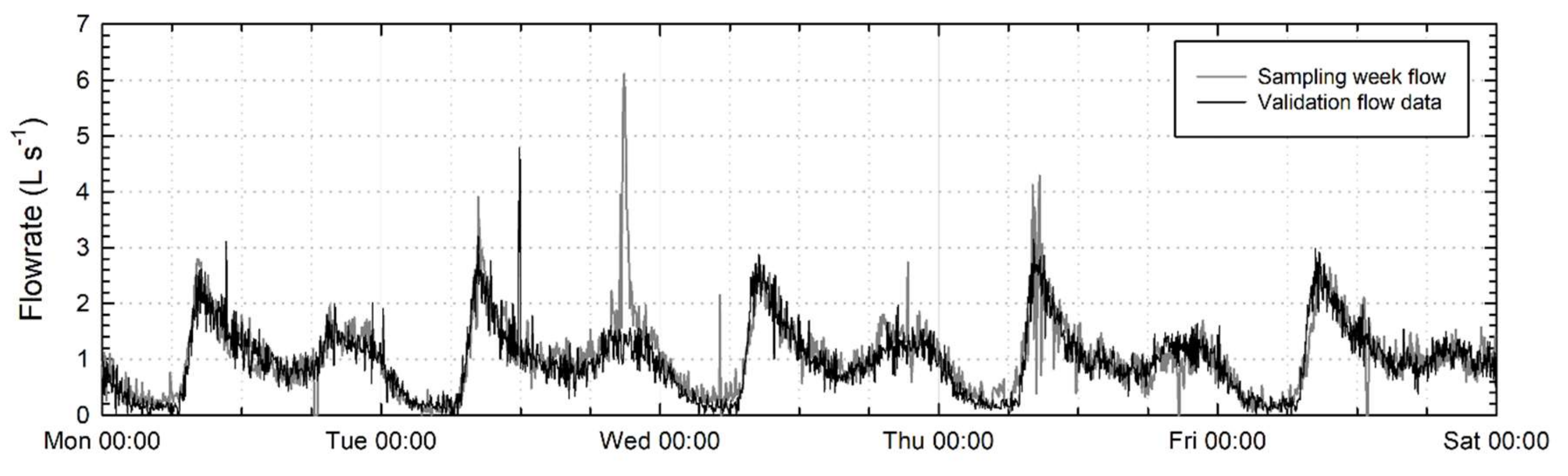
4.1. Calibration and Validation of the Stochastic Sewer Flow Model

Figure 5 shows the drinking water flow measured on entrance to the modelled catchment, demonstrating about a one-hour delay between clean water entering the catchment and the sewer flow leaving the catchment. This is due to a combination of time in flow and hold up time of water used in household appliances before discharge. Figure 5 also shows that in the early hours of the morning this delay extends to almost two hours, which is likely due to the longer hold-up derived from increased use of dishwashers and washing machines. The water balance between drinking water and wastewater data in Prinseneiland revealed an average excess of 1.3 m3 day−1 in the wastewater. This excess is likely due to infiltration to the sewer and runoff from the street and represents approximately 2% of the dry-weather flow. This external inflow to the system could also explain some of the difference between drinking water and wastewater flows, particularly at night when flow is low.
Once SIMDEUM® had been calibrated as described in Section 2.4.1, the model represented the sewer system described in Section 3 reasonably well. Comparison of the model output with the sewer flow data can be seen in Figure 6 along with the model evaluation statistics (correlation coefficient, Nash-Sutcliff coefficient and the root mean squared efficiency, R M S E ).
The model under-predicts the sewer flow during working hours, this is due to the assumption that the housing estate is purely domestic. There is an average discrepancy of 10 m3 between the hours of 10:00 and 18:00, which can be explained by the metered usage of the business premises. Nine percent of the registered properties on Prinseneiland are business addresses and these vary in function from warehouses to offices. These businesses were not modelled as they are not easy to describe well, and this study primarily investigates the impacts of varying water use on domestic wastewater.

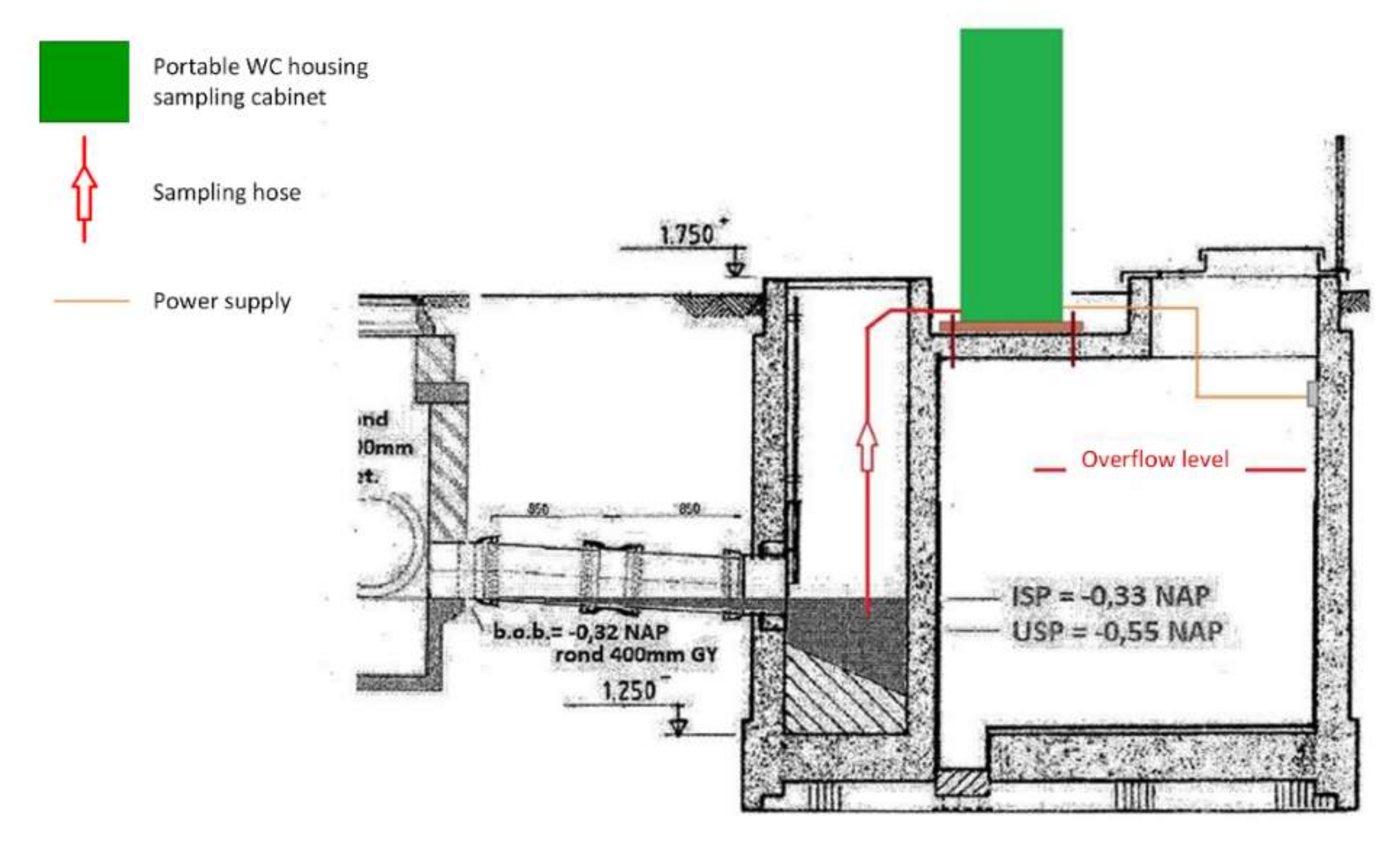
4.2. Sampling Wastewater for Quality Analysis

To confirm that the wastewater quality model provides a good representation of real life, a week-long wastewater sampling campaign was carried out, described in Section 2.4.2. The sampling campaign began on a Thursday at 11 am and ran through until the following Thursday at 11 am. These results have been reordered to represent a Monday–Friday profile for ease of analysis—but it should be noted that the Thursday and Friday measurements were taken the week before the Monday—Wednesday measurements. The weekends have not been modelled due to the limited capacity of SIMDEUM® to describe weekend water use. Weekend water use is less strongly linked to a daily routine and SIMDEUM® has yet to be developed to incorporate this difference. The results of the sampling campaign are shown in Figure 7, Figure 8 and Figure 9. Figure 7 shows how the measured wastewater flow over the sampling week compared to the measured wastewater flow used to validate the hydraulic model, see Section 4.1. There was heavy rainfall from 20:35 until 21:05 on the Tuesday evening of the sampling campaign; this explains the flow peak shown in Figure 7 (indicated by an arrow) and its deviation from the calibration flow. Figure 8; Figure 9 show the hourly measurements of wastewater concentration that were taken for total suspended solids (TSS), chemical oxygen demand (COD), total Kjeldahl nitrogen (TKN) and total phosphorus (TPH).
There was a good correlation between TSS and COD (R = 0.82) and a reasonable correlation between TKN and TPH (R = 0.55) but the correlation with suspended solids is weak (R = 0.38 for TKN and R = 0.20 for TPH). This indicates that the bulk of the COD is combined within the suspended solids but the TKN and TPH are present in a more dilute form. It is also notable that there is a reasonable correlation between the flowrate and the concentration of TSS and COD (R = 0.78 and R = 0.73 respectively). This seems to indicate that higher pollutant concentrations are produced at peak flow, but it is more likely that accumulated solids are washed through the system during high flow. This could be a consequence of sampling the wastewater downstream, where the highest concentration of COD/suspended solids occurs in the morning peak flow and the evening peak flow, but this is not necessarily the case upstream. This is discussed further in Section 4.3. TKN concentration also peaks with the morning surge in flow but then drops early afternoon, before steadily increasing throughout the evening until the next morning. TPH follows a very similar pattern to TKN but has a second evening peak in concentration. This is likely due to phosphorus sources now being restricted for the toilet and kitchen sink discharges, whereas the nitrogen is discharged more often.

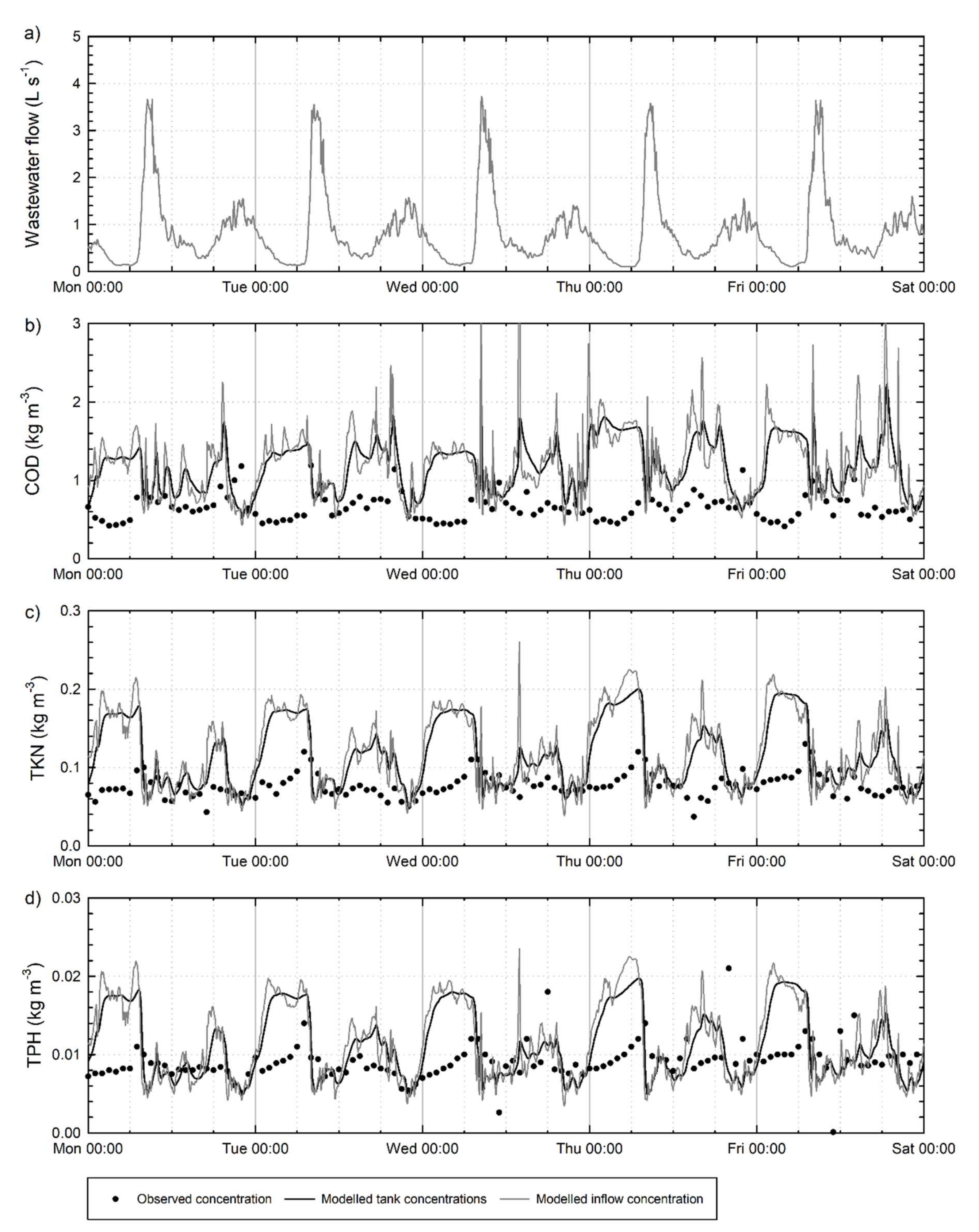
4.3. Model Comparison with Sewer Quality Data

Figure 10 shows a comparison of the modelled mass flow compared to the observed data (calculated as the product of the measured concentration and the measured wastewater flowrate). The shaded areas represent the sampling error associated with each parameter, highlighted in Table 2. As indicated in Section 4.2, there was heavy rainfall from 20:35 to 21:05 on the Tuesday evening of the sampling campaign, and this is reflected in the concentration peak on the second evening of the plots in Figure 10 (indicated by an arrow). Apart from this, the model represents the observed mass flow reasonably well, as the timing and magnitude of the mass flow profiles are in alignment with the measured values. The predicted mass flow overnight is, on average, higher than the observed mass flow, and the observed morning peak is higher than predicted. This confirms the hypothesis, in Section 4.2, that these flow peaks likely include accumulation of solids rather than higher concentration discharges from households. This build-up of suspended solids has not been accounted for in this version of the model as time-varying solid generation is not available in InfoWorks® (see Section 2.2).
Figure 11 shows the comparison of the predicted and measured nutrient concentration. The modelled tank concentrations were calculated according to Equation (3). This also supports the conclusion that the discrepancy between the modelled wastewater concentration and the observed is due to the lack of differential solids transport modelling in the network. The model predicts concentration to be highest during the night as most water use at night is from toilets, but this cannot be confirmed by the measured data. Following the design of the sampling campaign, the high concentration wastewater produced at night would only be accounted for during the first few 3-min sub-samples of the peak flow the following morning. The subsequent sub-samples are likely to be diluted substantially, leading to a morning peak in a lower concentration than the more concentrated night flows. SIMDEUM WW® appears to be performing well as a wastewater generator, but as the solids transport has not been adequately modelled within the sewer system (InfoWorks® ICM), the concentration cannot be aligned with the measured data. The modelled TKN and TPH follow the measured concentration data better than the COD, this is likely due to their lower correlation with suspended solids, and hence, dilute modelling is more appropriate here.

4.4. Variability of the Model

To address the variability of the stochastic model, each weekday was evaluated on factors of flow and nutrient mass—see Figure 12, where each day is compared to the first simulated day. The sample point for comparison was the final pipe of the network, before the pumping station. The stochastic model results are relatively consistent as the gradient of the line of best fit, m, for each day is close to 1. Correlation between Day 1 of the simulation and the subsequent days is very high for flowrate but the correlation is less strong for the nutrient mass flow. COD showed the smallest variability followed by TKN and then TPH. This is thought to be due to TKN and TPH being linked more strongly to appliances that follow a less strict daily usage pattern, e.g., kitchen taps, dishwashers and washing machines. Whereas the toilet and shower use (more strongly linked to COD generation) happen at similar times of day. Elias-Maxil [26] assessed the variability in SIMDEUM® with over 200 simulations and concluded that the pattern generator reaches a steady state after 75 simulations, i.e., the variability approaches zero. As the studied catchment includes 418 households, this confirms that the variability at the outfall is low.

4.5. Future Scenario Testing

Six future scenarios (Section 2.5) were tested using the stochastic flow and wastewater quality model to observe the effects of different water conservation technologies on flow and wastewater concentration. Increased wastewater concentration can offer benefits for resource recovery, whilst reducing household water use is beneficial for water security and sustainability reasons.
Figure 13 shows the results from this simulation, analysed over a 5-day period (Monday–Friday). It can be seen in Figure 13a, that the effect of Eco (2a/2b) and GWR (3a/3b) scenarios is the dramatic reduction in the morning peak. The sewer system experiences a much narrower range of flowrates in these scenarios, which warrants smaller pipe diameters. Penn, et al. [27] stated that for a 1–6 mm diameter solid, the critical shear is 0.867–1.42 Pa, respectively, so without reducing pipe diameters, these water use scenarios may struggle to transport larger solids (see Figure 13b).
Figure 13c–f shows the consequence on wastewater quality parameters, and there is little impact of population changes between the scenarios (a and b scenarios). RWH produces a very similar situation to the baseline as it is simply replacing potable sources with a non-potable alternative. The impact of this scenario is better addressed by evaluating the impact on the drinking water system, as it will likely increase water residence time in the distribution network, which may compromise water quality. The Eco scenario produces the highest concentration of wastewater, although the range of concentrations is similar to the baseline/RWH scenarios. GWR produces wastewater at concentrations between the other two scenarios but in a much narrower range. This scenario could, therefore, be preferable for resource recovery as there is a narrower operating range for treatment units. However, GWR is the poorest performing water use scenario in terms of wastewater temperature, as shower and bath water do not directly enter the sewer, hence sewer temperature reduces. This model has been demonstrated as a useful tool for analysis of various resource recovery options for future urban water planning.
Bailey et al. [13] concluded that this model over-predicts phosphorus concentrations, but with the results from the sampling campaign, and the changes made in the estimated wastewater composition due to the removal of phosphorus in detergents (Section 2.1.2), the model now predicts in line with reality. Daily pollutant load produced per capita in these scenarios ranged from 86–122 g COD, 8–12 g TKN and 0.8–1.2 g TPH—these values align with independently published values [21,28,29,30].

5. Conclusions

A new stochastic wastewater flow and quality model has been developed to address the impacts of water use changes on wastewater flow concentration. The hydraulic model was tested and validated in previous work. This paper presents the validation of the wastewater quality model using measured data. The model was used to investigate the impact of three water-saving strategies (greywater recycling, rainwater harvesting and installation of smart water appliances) on water quantity and quality in the sewer network.
The results obtained lead to the following key findings:
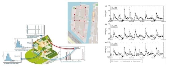
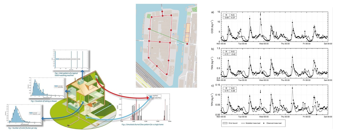
  • Stochastic sewer model wastewater quality validation: The predicted mass flows of COD, TKN and TPH compared well with the corresponding observed data values. The same, however, cannot be said for the COD, TKN and TPH concentrations. These concentrations were treated as dilute pollutants as InfoWorks® does not currently incorporate differential solids transport, leading to the misalignment of the predicted and measured concentration data. High concentration flows are produced by the stochastic generator during the night but only washed through the system in the morning. As the concentrations were measured at a downstream point in the network, there was a lag time in transporting suspended solids which was not accounted for in the network model.
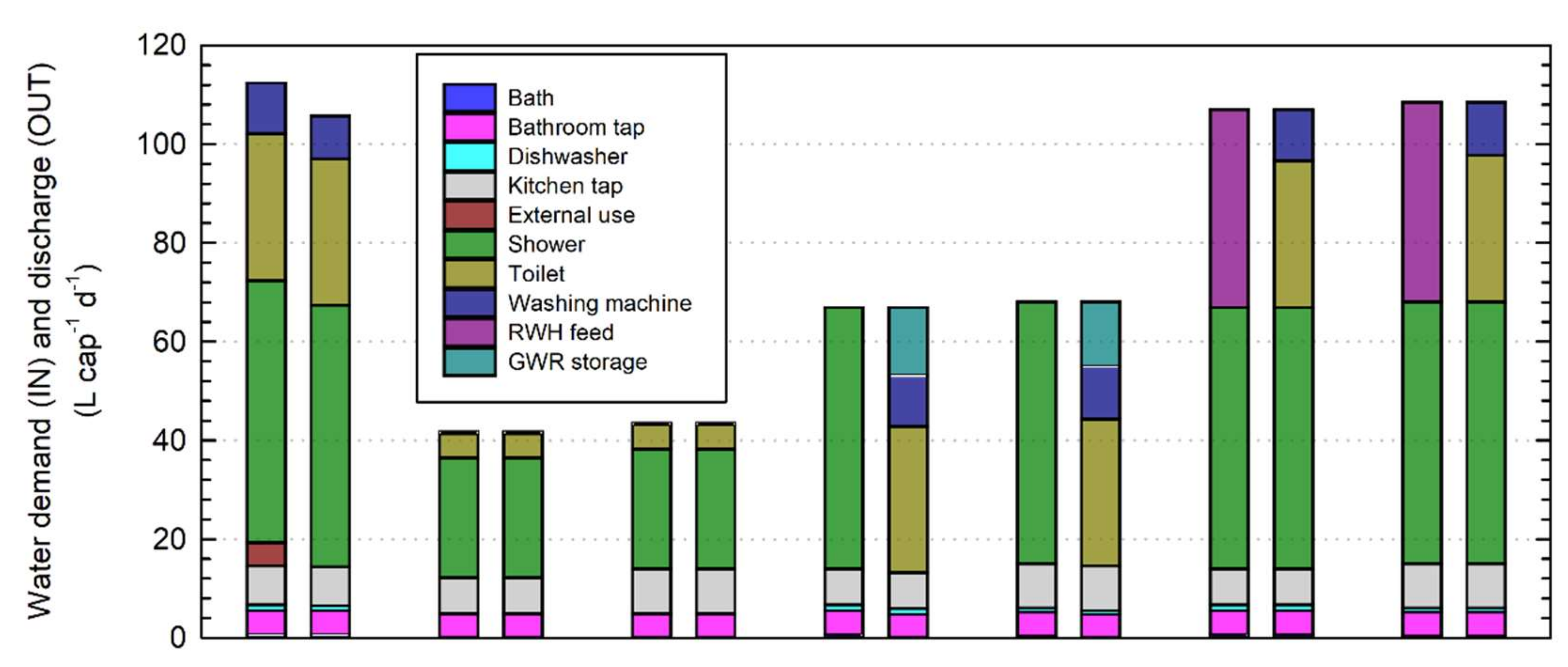
  • Implications for three water-saving strategies on the quantity and quality of flow in the receiving sewer network: It was found that wastewater flow can be reduced by up to 62% with concentrations of COD, TKN and TPH increasing by up to 111%, 84% and 75% respectively with the installation of water-saving appliances. In addition, it was found that the use of water-saving appliances and greywater recycling dramatically reduced the peak flows, whereas rainwater harvesting produced similar flow and concentration results in the baseline case. The greywater recycling case produced the most consistent wastewater concentrations and the lowest wastewater temperature.
  • Proposals for future work: This will involve incorporation of the time-varying component for suspended solids entry to the sewer system, and differential solids transport in the sewer. This advancement will be combined with a drinking water simulation to create a comprehensive urban water model for observing effects of future water use scenarios on the entire system. This project will ultimately highlight a future vision for the urban water cycle and support recommendations for optimal resource recovery within drinking and wastewater systems.

Supplementary Materials

The following are available online at https://www.mdpi.com/2073-4441/12/4/1187/s1

Author Contributions

Conceptualization, O.B., L.Z. and J.H.; Data curation, O.B.; Formal analysis, O.B. and L.Z.; Funding acquisition, J.P.v.d.H. and T.A.; Investigation, O.B.; Methodology, O.B. and L.Z.; Software, O.B., L.Z. and M.B.; Supervision, T.A. and J.H.; Validation, O.B. and L.Z.; Visualization, O.B. and J.H.; Writing—original draft, O.B.; Writing—review and editing, O.B., L.Z., J.P.v.d.H., Z.K., M.B., T.A. and J.H. All authors have read and agreed to the published version of the manuscript.

Funding

This study was conducted as part of the Water Informatics Science and Engineering (WISE) Centre for Doctoral Training (CDT), funded by the UK Engineering and Physical Sciences Research Council, Grant No. EP/L016214/1. Olivia Bailey is supported by a research studentship from this CDT. Funding was also obtained from the Topsector Water & Maritime TKI Watertechnology Program of the Dutch Ministry of Economic Affairs and Climate Change (No. 2016TUD003, project New Urban Water Transport Systems), water utility Waternet, drinking water companies Brabant Water, Limburg and Evides, water authority De Dommel, Amsterdam Institute for Advanced Metropolitan Solutions and Royal Haskoning DHV Consultancy.

Acknowledgments

The authors thank Waternet, the water utility of the city of Amsterdam, for providing expertise, data, and access to the sewer networks for field tests.

Conflicts of Interest

The authors declare no conflict of interest.

References

  1. Diamantis, V.; Verstraete, W.; Eftaxias, A.; Bundervoet, B.; Vlaeminck, S.E.; Melidis, P.; Aivasidis, A. Sewage pre-concentration for maximum recovery and reuse at decentralized level. Water Sci. Technol. 2013, 67, 1188–1193. [Google Scholar] [CrossRef] [PubMed]
  2. Mezohegyi, G.; Bilad, M.R.; Vankelecom, I.F.J. Direct sewage up-concentration by submerged aerated and vibrated membranes. Bioresour. Technol. 2012, 118, 1–7. [Google Scholar] [CrossRef] [PubMed]
  3. Bianchini, A.; Bonfiglioli, L.; Pellegrini, M.; Saccani, C. Sewage sludge drying process integration with a waste-to-energy power plant. Waste Manag. 2015, 42, 159–165. [Google Scholar] [CrossRef] [PubMed]
  4. Verstraete, W.; Vlaeminck, S.E. ZeroWasteWater: Short-cycling of wastewater resources for sustainable cities of the future. Int. J. Sustain. Dev. World Ecol. 2011, 18, 253–264. [Google Scholar] [CrossRef] [Green Version]
  5. Parkinson, J.; Schütze, M.; Butler, D. Modelling the impacts of domestic water conservation on the sustainability of the urban sewerage system. J. Chart. Inst. Water Environ. Manag. 2005, 19, 49–56. [Google Scholar] [CrossRef]
  6. Penn, R.; Hadari, M.; Friedler, E. Evaluation of the effects of greywater reuse on domestic wastewater quality and quantity. Urban Water J. 2012, 9, 137–148. [Google Scholar] [CrossRef]
  7. Penn, R.; Schütze, M.; Friedler, E. Modelling the effects of on-site greywater reuse and low flush toilets on municipal sewer systems. J. Environ. Manag. 2013, 114, 72–83. [Google Scholar] [CrossRef] [PubMed]
  8. Penn, R.; Schütze, M.; Gorfine, M.; Friedler, E. Simulation method for stochastic generation of domestic wastewater discharges and the effect of greywater reuse on gross solid transport. Urban Water J. 2017, 14, 846–852. [Google Scholar] [CrossRef]
  9. Watershare. Available online: https://www.watershare.eu/tool/water-use-info/ (accessed on 1 March 2020).
  10. Blokker, E.J.M.; Vreeburg, J.H.G.; van Dijk, J.C. Simulating Residential Water Demand with a Stochastic End-Use Model. J. Water Resour. Plan. Manag. 2010, 136, 19–26. [Google Scholar] [CrossRef]
  11. Pieterse-Quirijns, E.J.; Agudelo-Vera, C.M.; Blokker, E.J.M. Modelling sustainability in water supply and drainage with SIMDEUM®. In Proceedings of the CIBW062 Symposium, Melbourne, Australia, 8–10 September 2019. [Google Scholar]
  12. Bailey, O.; Arnot, T.C.; Blokker, E.J.M.; Kapelan, Z.; Vreeburg, J.; Hofman, J.A.M.H. Developing a stochastic sewer model to support sewer design under water conservation measures. J. Hydrol. 2019, 573, 908–917. [Google Scholar] [CrossRef] [Green Version]
  13. Bailey, O.; Arnot, T.C.; Blokker, E.J.M.; Kapelan, Z.; Hofman, J.A.M.H. Predicting impacts of water conservation with a stochastic sewer model. Water Sci. Technol. 2019, 80, 2148–2157. [Google Scholar] [CrossRef] [PubMed]
  14. Blokker, E.J.M. Stochastic Water Demand Modelling. In Hydraulics in Water Distribution Networks; IWA publishing: London, UK, 2011. [Google Scholar]
  15. Blokker, E.J.M.; Agudelo-Vera, C.A. Doorontwikkeling Simdeum: Waterverbruik over de dag, Energie voor Warmwater en Volume, Temperatuur en Nutriënten in Afvalwater; Report BTO 2015.210(s); KWR Water Research Institute: Nieuwegein, The Netherlands, 2015. [Google Scholar]
  16. Parkinson, J.N. Modelling Strategies for Sustainable Domestic Wastewater Management in a Residential Catchment; Imperial College for Science, Technology and Medicine: London, UK, 1999. [Google Scholar]
  17. Butler, D.; Friedler, E.; Gatt, K. Characterising the quantity and quality of domestic wastewater inflows. Water Sci. Technol. 1995, 31, 13. [Google Scholar] [CrossRef]
  18. Siegrist, R.; Witt, M.; Boyle, W. Characterisation of rural household wastewater. J. Environ. Eng. ASCE 1976, 102, 533–548. [Google Scholar]
  19. Surendran, S. Grey-water reclamation for non-potable re-use. J. CIWEM 1998, 12, 406–413. [Google Scholar] [CrossRef]
  20. The European Parliament; The Council of the European Union. Regulation (EU) No 259/2012 on the use of phosphates and other phosphorus compounds in consumer laundry detergents and consumer automatic dishwasher detergents. 2012. Available online: https://eur-lex.europa.eu/legal-content/EN/TXT/PDF/?uri=CELEX:32012R0259 (accessed on 1 March 2019).
  21. Comber, S.; Gardner, M.; Georges, K.; Blackwood, D.; Gilmour, D. Domestic source of phosphorus to sewage treatment works. Environ. Technol. 2013, 34, 1349–1358. [Google Scholar] [CrossRef] [PubMed] [Green Version]
  22. Ward, S.; Memon, F.A.; Butler, D. Harvested rainwater quality: The importance of building design. Water Sci. Technol. J. Int. Assoc. Water Pollut. Res. 2010, 61, 1707–1714. [Google Scholar] [CrossRef] [PubMed]
  23. Farreny, R.; Morales-Pinzón, T.; Guisasola, A.; Tayà, C.; Rieradevall, J.; Gabarrell, X. Roof selection for rainwater harvesting: Quantity and quality assessments in Spain. Water Res. 2011, 45, 3245–3254. [Google Scholar] [CrossRef] [PubMed]
  24. Agudelo, C.; Blokker, E.J.M. How Future Proof Is Our Drinking Water Infrastructure; Report BTO 2014.011; KWR Water Research Institute: Nieuwegein, The Netherlands, 2014. [Google Scholar]
  25. Waternet, Average Water Use. Available online: https://www.waternet.nl/en/our-water/our-tap-water/average-water-use/ (accessed on 1 March 2020).
  26. Elias-Maxil, J.A. Heat Modelling of Wastewater in Sewer Networks: Determination of Thermal Energy Content from Sewage with Modeling Tools; Technische Universiteit Delft: Delft, The Netherlands, 2015. [Google Scholar]
  27. Penn, R.; Schütze, M.; Friedler, E. Assessment of the effects of greywater reuse on gross solids movement in sewer systems. Water Sci. Technol. 2014, 69, 99–105. [Google Scholar] [CrossRef] [PubMed]
  28. Henze, M.; Loosdrecht, M.C.M.v.; Ekama, G.A.; Brdjanovic, D. 3 Wastewater Characterization. In Biological Wastewater Treatment—Principles, Modelling and Design; IWA Publishing: London, UK, 2008. [Google Scholar]
  29. Tchobanoglous, G.; Burton, F.L.; Stensel, H.D. Wastewater Engineering: Treatment, Disposal, and Reuse, 3rd ed.; Tchobanoglous, G., Burton, F.L., Eds.; McGraw-Hill: London, UK, 1991. [Google Scholar]
  30. Arildsen, A.L.; Vezzaro, L. Revurdering af Person Ækvivalent for Fosfor—Opgørelse af Fosforindholdet i Dansk Husholdningsspildevand i Årene fra 1990 til 2017. Kgs; Danmarks Tekniske Universitet (DTU): Lyngby, Denmark, 2019. [Google Scholar]
Figure 1. Wastewater sampling campaign equipment set up. Portable toilet housing the sampling cabinet that draws wastewater from the wet well of the pumping station in Prinseneiland. ISP is the level at which the pump switches on, USP is the level where the pump switches off. The tank area is 2 m2.
Water 12 01187 g001
Figure 2. Outline of appliance demand and discharge for each of the future scenarios.
Water 12 01187 g002
Figure 3. Map of modelled catchment—Prinseneiland, NL (Waternet, Amsterdam).
Water 12 01187 g003
Figure 4. Appliance-specific water use in Amsterdam, Netherlands [25] and the derived appliance usage of Prinseneiland assuming the Amsterdam average micro-component trend.
Water 12 01187 g004
Figure 5. Comparison of the mean drinking water and wastewater flow in the studied catchment.
Water 12 01187 g005
Figure 6. Performance of stochastic sewer model when compared to measured sewer flow data.
Water 12 01187 g006
Figure 7. Wastewater flow over sampling week compared to flow data used for model validation.
Water 12 01187 g007
Figure 8. Hourly concentration of suspended solids and chemical oxygen demand (COD) in wastewater over sampling week.
Water 12 01187 g008
Figure 9. Hourly concentration of total Kjeldahl nitrogen (TKN) and total phosphorus (TPH) in wastewater over sampling week.
Water 12 01187 g009
Figure 10. Mass flow of COD (a), TKN (b) and TPH (c) predicted by the model compared to the mass calculated from measured concentration and measured flow rate at the wastewater pumping station. The correlation coefficient (CC) and Nash–Sutcliff coefficient (N–S) are given for each plot.
Water 12 01187 g010
Figure 11. Wastewater flow (a) and modelled COD (b), TKN (c) and TPH (d) concentration in comparison with the measured concentration.
Water 12 01187 g011
Figure 12. (a) Variation in stochastic modelled flow over 5 days, (b) Flow variation over 5 days compared to Day 1, (c) COD mass flow variation over 5 days compared to Day 1, (d) TKN mass flow variation over 5 days compared to Day 1, (e) TPH mass flow variation over 5 days compared to Day 1.
Water 12 01187 g012
Figure 13. (a) Effect of scenarios on the flowrate at the catchment outfall, (bf) Cumulative frequency of the shear stress achieved, COD, Temperature, TKN and TPH concentration in wastewater at the catchment outfall over 5 day (respectively).
Water 12 01187 g013
Table 1. Appliance-specific pollutant concentrations for improved SIMDEUM WW® (adapted from Bailey et al. [13]). Bold values were defined in this work using observed wastewater data.
ApplianceTemperature (°C)Sewage Quality (g use−1)Ref.
CODTKNTPHTSS
Bath3625.900.850.008.88[5,16]
Shower3512.600.490.004.32[5,16]
Bathroom tap401.480.040.000.56[5,16]
Kitchen tap407.480.350.034.68[5,16,21]
Dish washer35301.350.0013.20[5,16]
Washing machine
-
With GWR
-
With RWH
(35, 35, 35, 45)65.250.6380.0017.10[5,16]
69.400.780.0017.88[6]
66.290.860.0017.72[22]
Toilet
-
With GWR
-
With RWH
2311.221.990.223.04[15,21]
11.482.000.223.09[6]
11.282.000.223.08[22]
Table 2. Wastewater quality parameters analysed and specific methodology associated with each parameter.
Parameter SampledParameter DescriptionMethod (Eurofins Omegam)Limit of Determination
(mg l−1)
Required Sample Volume
(ml Sample−1)
Measurement Uncertainty (+/−)
COD (mg l−1)Chemical oxygen demandConforms to NEN 66335.0010015%
TKN (mg l−1)Total Nitrogen-KjeldahlConforms to NEN-ISO 56631.0010013%
TPH (mg l−1)Total PhosphorusOwn method based on NEN-EN-ISO 15681_20.055012%
TSS (mg l−1)Total suspended solidsConforms to NEN-EN 872 and NEN 64991.0075016%
Table 3. Future scenario description.
ScenarioDemand (L cap−1 d−1)Description
1—Baseline112Present-day scenario—validated hydraulic model
2a—Eco, max. occupancy42Water-saving appliances such as 1 L flush toilets and water-saving showers (as presented by Agudelo and Blokker [24])
2b—Eco, min. occupancy44
3a—GWR, max. occupancy67Greywater reuse utilised for toilet flushing and washing machines
3b—GWR, min. occupancy68
4a—RWH, max. occupancy67Rainwater harvesting utilised for toilet flushing and washing machines
4b—RWH, min. occupancy68
Table 4. Population statistics for present and future scenarios (based data and projections obtained from Gemeente Amsterdam).
SingleDualFamilyFamily SizeOccupancy
Baseline58%23%19%3.41.7
(a) Max.55%21%24%3.51.8
(b) Min.91% 4% 5%3.11.1
(a) Amsterdam projected population statistics, (b) Reduction in average occupancy to 1.1.

