Assessment of Ecological and Hydro-Geomorphological Alterations under Climate Change Using SWAT and IAHRIS in the Eo River in Northern Spain

 ,
,  ,
,
Abstract
:
1. Introduction
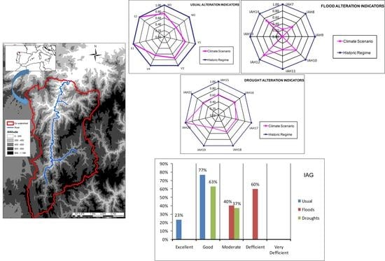
2. Study Area
3. Materials and Methods
3.1. SWAT Model
3.2. Model Set Up and Data Sets
3.3. Sensitivity Analysis, Calibration and Validation
3.4. Goodness-of-Fit Tests
3.5. Climate Change Scenarios
3.6. IAHRIS
4. Results and Discussion
4.1. Meteorological Variations under Climate Change Scenarios
4.2. Sensitivity Analysis, Calibration and Validation of the SWAT Model
4.3. Model Performance
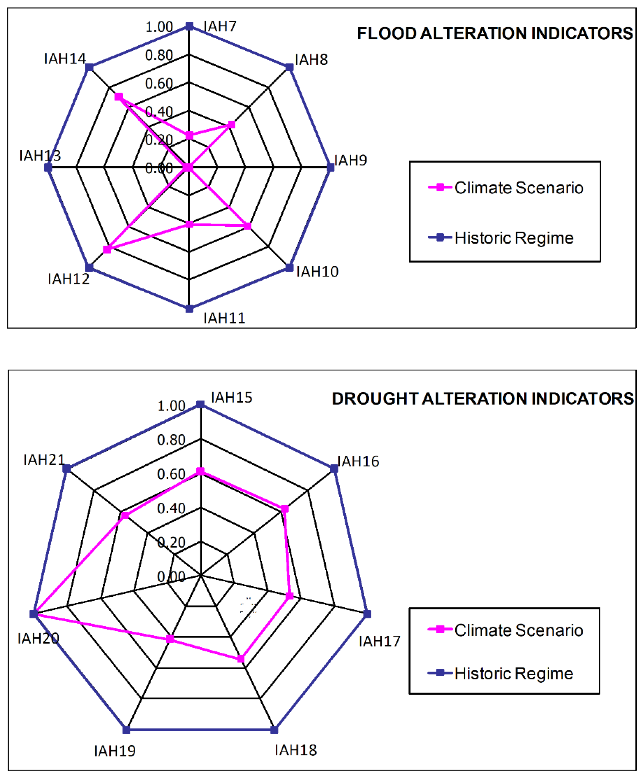
4.4. Variations in Streamflow
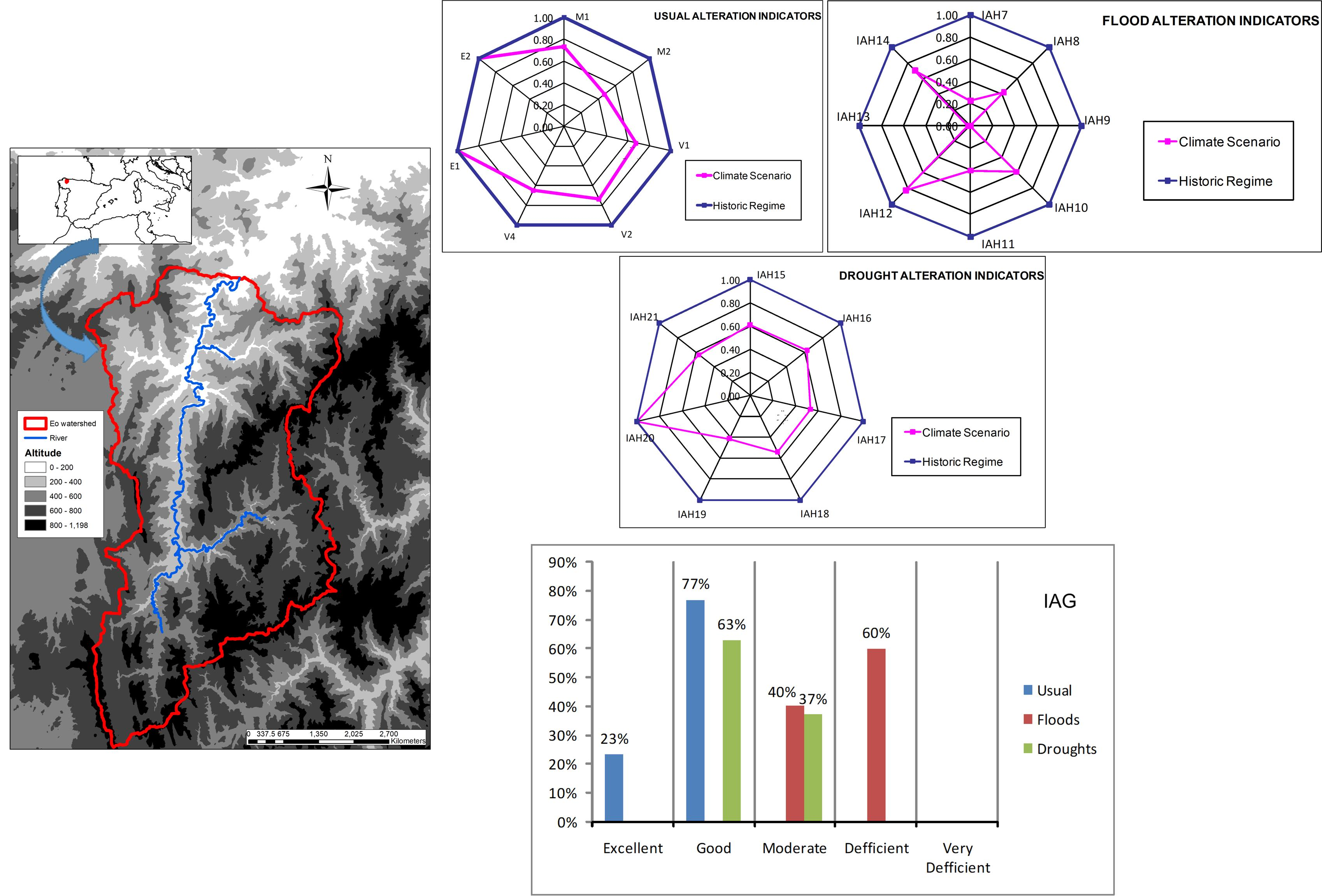
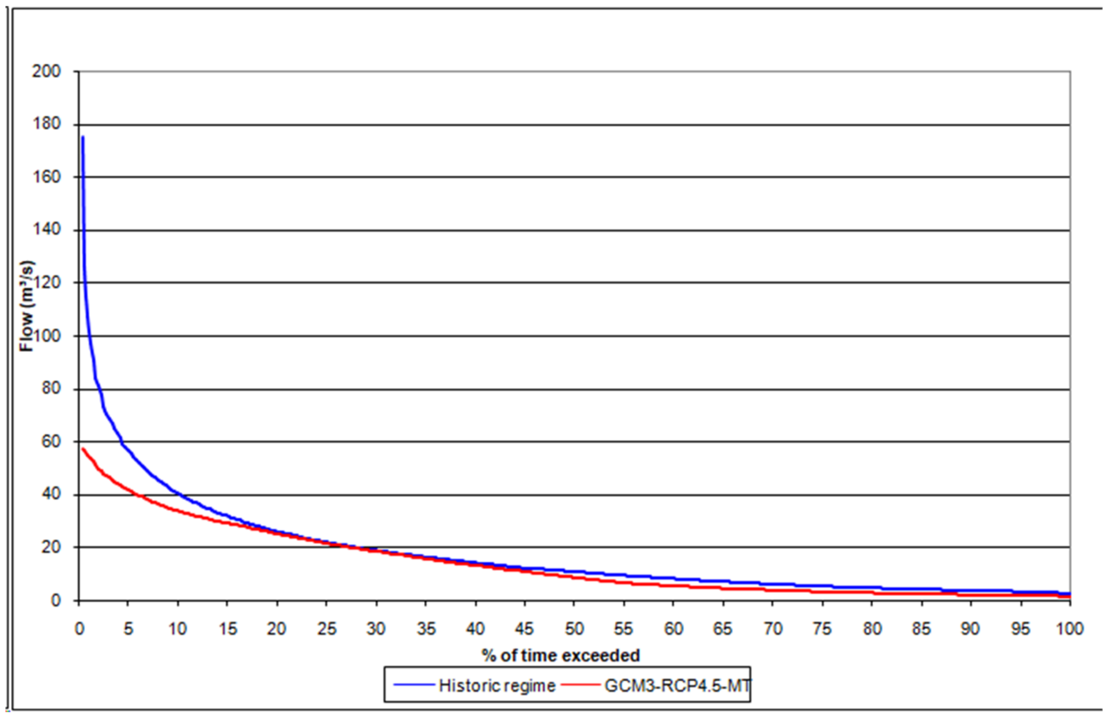
4.5. IAHRIS
5. Conclusions
Author Contributions
Funding
Conflicts of Interest
Appendix A. IAHRIS Methodology
References
- Naiman, R.J.; Bunn, S.E.; Nilsson, C.; Petts, G.E.; Pinay, G.; Thompson, L.C. Legitimizing fluvial systems as users of water: An overview. Environ. Manag. 2002, 30, 455–467. [Google Scholar] [CrossRef] [PubMed]
- EC (European Communities). Directive 2000/60/EC of the European Parliament and of the Council of 23 October 2000 establishing a framework for community action in the field of water policy. Off. J. Eur. Comm. 2000, 22, 2000. [Google Scholar]
- Belletti, B.; Rinaldi, M.; Buijse, A.D.; Gurnell, A.M.; Mosselman, E. A review of assessment methods for river hydromorphology. Environ. Earth Sci. 2015, 73, 2079–2100. [Google Scholar] [CrossRef]
- Poff, N.L.; Allan, J.D.; Bain, M.B.; Karr, J.R.; Prestegaard, K.L.; Richter, B.D.; Stromberg, J. The Natural Flow Regime. A paradigm for river conservation and restoration. Bioscience 1997, 47, 769–784. [Google Scholar] [CrossRef]
- Richter, B.D.; Baumgartner, J.V.; Braun, D.P.; Powell, J. A spatial assessment of hydrologic alteration within a river network. Regul. Rivers Res. Manag. 1998, 14, 329–340. [Google Scholar] [CrossRef]
- Arthington, A.H. Wounded Rivers, Thirsty Land: Getting Water Management Right; Inaugural Professorial Lecture; Griffith University: Brisbane, SEQ, Australia, 1997. [Google Scholar]
- Bunn, S.E.; Arthington, A. Basic principles and ecological consequences of altered flow regimes for aquatic biodiversity. Environ. Manag. 2002, 30, 492–507. [Google Scholar] [CrossRef] [Green Version]
- Richter, B.D.; Baumgartner, J.V.; Powell, J.; Braun, D.P. A method for Assessing Hydrologic Alteration within Ecosystems. Conserv. Biol. 1996, 10, 1163–1174. [Google Scholar] [CrossRef] [Green Version]
- Lytle, D.H.; Poff, N.L. Adaptation to Natural Flow Regimes. Trends Ecol. Evol. 2004, 19, 94–100. [Google Scholar] [CrossRef]
- Gleick, P.H. The Status of Large Dams: The End of an Era? In The World’s Water 1998–1999: The Biennial Report on Freshwater Resources; Gleick, P.H., Ed.; Island Press: Washington, DC, USA, 1998; pp. 69–104. [Google Scholar]
- Arthington, A.H.; Naiman, R.J.; McClain, M.E.; Nilsson, C. Pre-serving the biodiversity and ecological services of rivers: New challenges and research opportunities. Freshw. Biol. 2010, 55, 1–16. [Google Scholar] [CrossRef] [Green Version]
- Poff, N.L.; Olden, J.D.; Merritt, D.M.; Pepin, D.M. Homogenization of regional river dynamics by dams and global biodiversity implications. Proc. Natl. Acad. Sci. USA 2007, 104, 5732–5737. [Google Scholar] [CrossRef] [Green Version]
- Döll, P.; Fiedler, K.; Zhang, J. Global-RCPale analysis of river flow alterations due to water withdrawals and reservoirs. Hydrol. Earth Syst. Sci. 2009, 13, 2413–2432. [Google Scholar] [CrossRef] [Green Version]
- Carlisle, D.M.; Wolock, D.M.; Meador, M.R. Alteration of streamflow magnitudes and potential ecological consequences: A multiregional assessment. Front. Ecol. Environ. 2011, 9, 264–270. [Google Scholar] [CrossRef]
- Martínez Fernández, J.; Fitz, C.; Esteve Selma, M.A.; Guaita, N.; Martínez-López, J. Modelling the effects of land use change on the nutrient dynamics in a coastal agricultural watershed: The Mar Menor case (Southeastern Spain). Ecosistemas 2013, 22, 84–94. [Google Scholar] [CrossRef] [Green Version]
- Schneider, C.; Laizé, C.L.R.; Acreman, M.C.; Flörke, M. How will climate change modify river flow regimes in Europe? Hydrol. Earth Syst. Sci. 2013, 17, 325–339. [Google Scholar] [CrossRef] [Green Version]
- IPCC. Climate Change 2014: Synthesis Report; Contribution of Working Groups I, II and III to the Fifth Assessment Report of the Intergovernmental Panel on Climate Change; Pachauri, R.K., Meyer, L.A., Eds.; IPCC: Geneva, Switzerland, 2014. [Google Scholar]
- IPCC. Climate Change 2001: The Scientific Basis; Contribution of Working Group I to the third assessment report of the Intergovernmental Panel on climate change; Houghton, J.T., Ding, Y., Griggs, D.J., Noguer, M., Van Der Linden, P.J., Dai, X., Maskell, K., Johnson, C.A., Eds.; Cambridge University Press: Cambridge, UK, 2001. [Google Scholar]
- IPCC. Climate Change 2007: Synthesis Report; Contribution of Working Groups I, II and III to the Fourth Assessment Report of the Intergovernmental Panel on Climate Change; Pachauri, R.K., Reisinger, A., Eds.; IPCC: Geneva, Switzerland, 2007. [Google Scholar]
- IPCC. Climate Change 2013: The Physical Science Basis; Contribution of Working Group I to the Fifth Assessment Report of the Intergovernmental Panel on Climate Change; Stocker, T.F., Qin, D., Plattner, G.-K., Tignor, M., Allen, S.K., Boschung, J., Nauels, A., Xia, Y., Bex, V., Midgley, P.M., Eds.; Cambridge University Press: Cambridge, UK, 2013. [Google Scholar]
- Rodríguez, R.; Navarro, X.; Casas, M.C.; Ribalaygua, J.; Russo, B.; Pouget, L.; Redano, A. Influence of climate change on IDF curves for the metropolitan area of Barcelona (Spain). Int. J. Climatol. 2014, 34, 643–654. [Google Scholar] [CrossRef] [Green Version]
- Pfeiffer, M.; Ionita, M. Assessment of Hydrologic Alterations in Elbe and Rhine Rivers, Germany. Water 2017, 9, 684. [Google Scholar] [CrossRef] [Green Version]
- Fotovatikhah, F.; Herrera, M.; Shamshirband, S.; Chau, K.; Ardabili, S.F.; Piran, J. Survey of computational intelligence as basis to big flood management: Challenges, research directions and future work. Eng. Appl. Comput. Fluid Mech. 2018, 12, 411–437. [Google Scholar] [CrossRef] [Green Version]
- Saiful Islam, A.K.M.; Supria, P.; Khaled, M.; Mutasim, B.; Golam Rabbani, F.; Alfi, H.; Tarekul Islam, G.M.; Sujit Kumar, B. Hydrological response to climate change of the Brahmaputra basin using CMIP5 general circulation model ensemble. J. Water Clim. Change 2018, 9, 434–448. [Google Scholar] [CrossRef]
- Homsi, R.; Sanusi Shiru, M.; Shahid, S.; Ismail, T.; Bin Harun, S.; Al-Ansari, N.; Chau, K.; Mundher Yaseen, Z. Precipitation projection using a CMIP5 GCM ensemble model: A regional investigation of Syria. Eng. Appl. Comput. Fluid Mech. 2020, 14, 90–106. [Google Scholar] [CrossRef]
- Manabe, S.; Wetherald, R.T. Large Scale changes of soil wetness induced by an increase in atmospheric carbon dioxide. J. Atmos. Sci. 1987, 44, 1211–1235. [Google Scholar] [CrossRef] [Green Version]
- Roads, J.O.; Marshall, S.; Oglesby, R.; Chen, S.C. Sensitivity of the CCM! Hydrologic cycle to CO2. J. Geophys. Res. 1996, 101, 7321–7339. [Google Scholar] [CrossRef]
- Arora, V.K.; Boer, G.J. Effects of simulated climate change on the hydrology of major river basins. J. Geophys. Res. 2001, 106, 3335–3348. [Google Scholar] [CrossRef]
- Iglesias, A.; Estrela, T.; Gallart, F. Impactos sobre los recursos hídricos. In Impactos del Cambio Climático en España; Ministerio de Medio Ambiente: Madrid, Spain, 2005; pp. 303–353. [Google Scholar]
- Benito, G.; Machado, M.J.; Pérez-González, A. Climate change and flood sensitivity in Spain. In Global Continental Changes: The Context of Palaeohydrology; Geological Society of London Special Publication 115; Branson, J., Brown, A.G., Gregory, K.J., Eds.; The Geological Society: London, UK, 1996; pp. 85–98. [Google Scholar]
- Blackwell, M.S.A.; Maltby, E. Ecoflood Guidelines: How to Use Floodplains for Flood Risk Reduction; Ecoflood Project; European Commision: Brussels, Belgium, 2006. [Google Scholar]
- Lee, A.; Cho, S.; Kang, D.K.; Kim, S.D. Analysis of the effect of climate change on the Nakdong river stream flow using indicators of hydrological alteration. J. Hydro Environ. Res. 2014. [Google Scholar] [CrossRef]
- Choi, D.; Lee, J.; Jo, D.; Kim, S. GCMs evaluation focused on Korean climate reproducibility. J. Korean Soc. Water Qual. 2010, 26, 482–490. [Google Scholar]
- Randall, D.A.; Wood, R.A.; Bony, S.; Colman, R.; Fichefet, T.; Fyfe, J.; Kattsov, V.; Pitman, A.; Shukla, J.; Srinivasan, J.; et al. Climate Models and Their Evaluation. In Climate Change 2007: The Physical Science Basis; Contribution of Working Group I to the Fourth Assessment Report of the Intergovernmental Panel on Climate Change; Solomon, S., Qin, D., Manning, M., Chen, Z., Marquis, M., Averyt, K.B., Tignor, M., Miller, H.L., Eds.; Cambridge University Press: Cambridge, UK; New York, NY, USA, 2007. [Google Scholar]
- Moss, R.H.; Edmonds, J.A.; Hibbard, K.A.; Manning, M.R.; Rose, S.K. The next generation of Scenarios for climate change research and assessment. Nature 2010, 463, 747–756. [Google Scholar] [CrossRef]
- Gao, Y.; Vogel, R.M.; Kroll, C.N.; Poff, N.L.; Olden, J.D. Development of representative indicators of hydrologic alteration. J. Hydrol. 2009, 374, 136–147. [Google Scholar] [CrossRef]
- Olden, J.D.; Poff, N.L. Redundancy and the choice of hydrologic indices for characterizing streamflow regimes. River Res. Appl. 2003, 19, 101–121. [Google Scholar] [CrossRef]
- Yang, Z.; Yan, Y.; Liu, Q. Assessment of the flow regime alterations in the Lower Yellow River, China. Ecol. Inform. 2012, 10, 56–64. [Google Scholar] [CrossRef]
- Opperman, J. Preliminary IHA Analysis for the Middle Fork Willamette River at Jasper OR. 2006. Available online: https://www.conservationgateway.org/Documents/Jasper%20IHA%20analysis.pdf (accessed on 22 August 2019).
- Opperman, J. Indicators of Hydrologic Alteration Analysis for the Patuca River. 2006. Available online: https://www.conservationgateway.org/Documents/Patuca%20IHA%20report%20v2.pdf (accessed on 12 April 2019).
- Faye, C. Characterization of the effects of manantali dam on the hydrological regime of the Senegal river by the IHA/RVA method. Open Access J. Sci. 2018, 2, 387–390. [Google Scholar] [CrossRef]
- Lin, K.; Zhang, F.; Zhang, Q.; Tu, X.; Hu, Y. Fuzzy-Based Comprehensive Evaluation of Environmental Flow Alteration. In Hydrologic Modeling; Water Science and Technology Library; Singh, V., Yadav, S., Yadava, R., Eds.; Springer: Singapore, 2018; Volume 81, pp. 621–638. [Google Scholar]
- Yuqin, G.; Pandey, K.P.; Huang, X.; Suwal, N.; Bhattarai, K.P. Estimation of Hydrologic Alteration in Kaligandaki River Using Representative Hydrologic Indices. Water 2019, 11, 688. [Google Scholar] [CrossRef] [Green Version]
- Laizé, C.L.R.; Acreman, M.; Schneider, C.; Dunbar, M.J.; Houghton-Carr, H.A.; Flörke, M.; Hannah, D.M. Projected flow alteration and ecological risk for pan-European rivers. River Res. Appl. 2014, 30, 299–314. [Google Scholar] [CrossRef] [Green Version]
- Stagl, J.C.; Hattermann, F.F. Impacts of Climate Change on the Hydrological Regime of the Danube River and Its Tributaries Using an Ensemble of Climate Scenarios. Water 2015, 7, 6139–6172. [Google Scholar] [CrossRef]
- Krysanova, V.; Hattermann, F.F.; Huang, S.H.; Hesse, C.; Vetter, T.; Liersch, S.; Koch, H.; Kundzewicz, Z.W. Modelling climate and land-use change impacts with SWIM: Lessons learnt from multiple applications. Hydrolog. Sci. J. 2015, 60, 606–635. [Google Scholar] [CrossRef]
- Chatterjee, S.; Daniels, M.D.; Sheshukov, A.Y.; Gao, J. Projected climate change impacts on hydrologic flow regimes in the Great Plains of Kansas. River Res. Appl. 2018, 34, 195–206. [Google Scholar] [CrossRef]
- European Comission. Ecological Flows in the Implementation of the Water Framework Directive. EC CIS Guidance Document nº31. 2015. Available online: https://circabc.europa.eu/sd/a/4063d635-957b-4b6f-bfd4-b51b0acb2570/Guidance%20No%2031%20-%20Ecological%20flows%20%28final%20version%29.pdf (accessed on 11 March 2020).
- Martinez Santa-María, C.; Fernández-Yuste, J.A. IAHRIS 2.2. Indicators of Hydrologic Alteration in Rivers. Methodological Reference Manual & User’s Manual. 2010. Available online: http://www.ecogesfor.org/IAHRIS_es.html (accessed on 26 October 2019).
- CEDEX. Índices de Alteración Hidrológica en Ríos. 2019. Available online: http://ambiental.cedex.es/hidromorfologia-iahris.php (accessed on 28 July 2019).
- Fernández-Yuste, J.; Martínez Santa-María, C.; Magdaleno, F. Application of indicators of hydrologic alterations in the designation of heavily modified water bodies in Spain. Environ. Sci. Policy 2012, 16, 31–43. [Google Scholar] [CrossRef]
- Magdaleno, F.; Donadio, C.; Kondolf, G.M. 30-year response to damming of a Mediterranean river in California, USA. Phys. Geogr. 2018, 39, 197–215. [Google Scholar] [CrossRef]
- Martinez Santa-Maria, C.; Fernández-Yuste, J.A. Obtención de escenarios de régimen ambiental de caudales (RAC) a partir del régimen natural: Una nueva extensión del software IAHRIS. In Proceedings of the I Congreso Ibérico de Restauración Fluvial—RestauraRíos, León, Spain, 18–20 October 2013. [Google Scholar]
- Lopes, J.S. Application of Indicators of Hydrologic Alteration in Portuguese Rivers Impacted by Dams. Master’s Thesis, Instituto Superior Técnico, Lisbon University, Lisbon, Portugal, 2013. [Google Scholar]
- Fernandez-Yuste, J.A.; Martinez Santa-Maria, C.; Sanchez, F.J.; Magdaleno, F.; Andres, A. IAHRIS: A new software to evaluate hydrologic alteration. In Proceedings of the 4th ECCR International Conference on River Restoration, Venice, Italy, 16–19 June 2008; pp. 981–991. [Google Scholar]
- Fernandes, M.R.; Segurado, P.; Jauch, E.; Ferreira, M.T. Riparian responses to extreme climate and land-use change Scenarios. Sci. Total Environ. 2016, 569, 145–158. [Google Scholar] [CrossRef]
- Chase, J.W.; Benoy, G.A.; Hann, S.W.R.; Culp. J.M. Small differences in riparian vegetation significantly reduce land use impacts on stream flow and water quality in small agricultural watersheds. J. Soil Water Conserv. 2016, 71, 194–205. [Google Scholar] [CrossRef]
- Aguiar, F.C.; Martins, M.J.; Cristiano, P.; Maria, S.; Fernandes, R. Riverscapes downstream of hydropower dams: Effects of altered flows and historical land-use change. Landsc. Urban Plan. 2016, 153, 83–98. [Google Scholar] [CrossRef]
- Cheng, J.; Xu, L.; Wang, X.; Jiang, J.; You, H. Assessment of hydrologic alteration induced by the Three Gorges Dam in Dongting Lake, China. River Res. Appl. 2018, 34, 686–696. [Google Scholar] [CrossRef]
- Zhang, Z.; Huang, Y.; Huang, J. Hydrologic Alteration Associated with Dam Construction in a Medium-Sized Coastal Watershed of Southeast China. Water 2016, 8, 317. [Google Scholar] [CrossRef] [Green Version]
- Gao, B.; Li, J.; Wang, X. Analyzing Changes in the Flow Regime of the Yangtze River Using the Eco-Flow Metrics and IHA Metrics. Water 2018, 10, 1552. [Google Scholar] [CrossRef] [Green Version]
- CHCO. Plan Hidrológico de la Demarcación Hidrográfica del Cantábrico Occidental 2015–2021. 2019. Available online: https://www.chcantabrico.es/dhc-occidental (accessed on 30 May 2019).
- Arnold, J.G.; Srinivasan, R.; Muttiah, R.S.; Williams, J.R. Large area hydrologic modeling and assessment part I: Model development. JAWRA J. Am. Water Resour. Assoc. 1998, 34, 73–89. [Google Scholar] [CrossRef]
- Krysanova, V.; Arnold, J.G. Advances in ecohydrological modelling with SWAT—A review. Hydrol. Sci. J. 2008, 53, 939–947. [Google Scholar] [CrossRef]
- Francesconi, W.; Srinivasan, R.; Pérez-Miñana, E.; Willcock, S.P.; Quintero, M. Using the Soil and Water Assessment Tool (SWAT) to model ecosystem services: A systematic review. J. Hydrol. 2016, 535, 625–636. [Google Scholar] [CrossRef]
- Tam, N.V.; Jörg, D. Modification of the SWAT model to simulate regional groundwater flow using a multicell aquifer. Hydrol. Process. 2018, 32, 939–953. [Google Scholar]
- Glavan, M.; Pintar, M. Strengths, Weaknesses, Opportunities and Threats of Catchment Modelling With Soil and Water Assessment Tool (Swat) Model. 2012. Available online: http://www.intechopen.com/articles/show/title/strengths-weaknesses-opportunities-and-threats-of-catchment-modelling-with-soil-and-water-assessment (accessed on 26 May 2020).
- Herrera, S.; Fernández, J.; Gutiérrez, J.M. Update of the Spain02 gridded observational dataset for EURO-CORDEX evaluation: Assessing the effect of the interpolation methodology. Int. J. Climatol. 2016, 36, 900–908. [Google Scholar] [CrossRef] [Green Version]
- Metalocus. HSC Hydrographical Study Centre. 2019. Available online: https://www.metalocus.es/en/news/hydrographic-studies-center-miguel-fisac (accessed on 18 February 2019).
- Dile, Y.T.; Daggupati, P.; George, C.; Srinivasan, R.Y.; Arnold, J. Introducing a new open source GIS user interface for the SWAT model. Environ. Model. Soft. 2016, 85, 129–138. [Google Scholar] [CrossRef]
- Hargreaves, G.H. Defining and using reference evapotranspiration. J. Irrig. Drain. E-ASCE 1994, 120, 1132–1139. [Google Scholar] [CrossRef]
- Nachtergaele, F.; van Velthuizen, H.; Verelst, L.; Batjes, N.; Dijkshoorn, K.; van Engelen, V.; Fischer, G.; Jones, A.; Montanarella, L.; Petri, M. Harmonized World Soil Database; Food and Agriculture Organization of the United Nations: Rome, Italy, 2008. [Google Scholar]
- Abbaspour, K.C. SWAT Calibration and Uncertainty Program—A User Manual; SWAT-CUP-2012; Swiss Federal Institute of Aquatic Science and Technology: Dubendorf, Switzerland, 2012. [Google Scholar]
- Nash, J.E.; Sutcliffe, J.V. River flow forecasting through conceptual models. Part I: A discussion of principles. J. Hydrol. 1970, 10, 282–290. [Google Scholar] [CrossRef]
- Kalin, L.; Isik, S.; Schoonover, J.E.; Lockaby, B.G. Predicting water quality in unmonitored watersheds using Artificial Neural Networks. J. Environ. Qual. 2010, 39, 1429–1440. [Google Scholar] [CrossRef] [PubMed]
- Burke, E.J.; Perry, R.H.J.; Brown, S.J. An extreme value analysis of UK drought and projections of change in the future. J. Hydrol. 2010, 388, 131–143. [Google Scholar] [CrossRef]
- Vaghefi, S.A.; Abbaspour, N.; Kamali, B.; Abbaspour, K.C. A toolkit for climate change analysis and pattern recognition for extreme weather conditions—Case study: California-Baja California Peninsula. Environ. Model. Softw. 2017, 96, 181–198. [Google Scholar] [CrossRef]
- Teutschbein, C.; Seibert, J. Bias correction of regional climate model simulations for hydrological climate-change impact studies: Review and evaluation of different methods. J. Hydrol. 2012, 456, 12–29. [Google Scholar] [CrossRef]
- Hempel, S.; Frieler, K.; Warszawski, L.; Rschewe, J.; Piontek, F. A trend-preserving bias correction—The ISI-MIP approach. Earth Syst. Dyn. 2013, 4, 219–236. [Google Scholar] [CrossRef] [Green Version]
- Pulido-Velazquez, D.; García-Aróstegui, J.L.; Molina, J.L.; Pulido-Velazquez, M. Assessment of future groundwater recharge in semi-arid regions under climate change scenarios (Serral-Salinas aquifer, SE Spain). Could increase rainfall variability increase the recharge rate? Hydrol. Process. 2015, 29, 828–844. [Google Scholar] [CrossRef]
- Blanco-Gómez, P.; Jimeno-Sáez, P.; Senent-Aparicio, J.; Pérez-Sánchez, J. Impact of Climate Change on Water Balance Components and Droughts in the Guajoyo River Basin (El Salvador). Water 2019, 11, 2360. [Google Scholar] [CrossRef] [Green Version]
- Directorate General Environment of the European Commission. WFD CIS Guidance Document No. 5. In Rivers and Lakes—Typology, Reference Conditions and Classification Systems; Directorate General Environment of the European Commission: Brussels, Belgium, 2003. [Google Scholar]
- Ribalaygua, J.; Pino, M.R.; Pórtoles, J.; Roldán, E.; Gaitán, E.; Chinarro, D.; Torres, L. Climate change scenarios for temperature and precipitation in Aragón (Spain). Sci. Total Environ. 2013, 463, 1015–1030. [Google Scholar] [CrossRef]
- Jimeno-Sáez, P.; Senent-Aparicio, J.; Pérez-Sánchez, J.; Pulido-Velazquez, D. A Comparison of SWAT and ANN Models for Daily Runoff Simulation in Different Climatic Zones of Peninsular Spain. Water 2018, 10, 192. [Google Scholar] [CrossRef] [Green Version]
- Neto, J.O.M.; Silva, A.A.; Mello, C.R.; Júnior, A.V.M. Simulação Hidrológica escalar com o modelo SWAT. Revista Brasileira Recursos Hídricos 2014, 19, 177–188. [Google Scholar] [CrossRef]
- Pinto, D.B.F.; Silva, A.M.; Beskow, S.; Mello, C.R.; Coelho, G. Application of the soil and water assessment tool (SWAT) for sediment transport simulation at a headwater watershed in Minas Gerais state, Brazil. Trans. ASABE 2013, 56, 697–709. [Google Scholar]
- Andrade, M.A.; Mello, C.R.; Beskow, S. Simulação hidrológica em uma bacia hidrográfica representativa dos Latossolos na região Alto Rio Grande, MG. Rev. Bras. Eng. Agric. Ambient. 2013, 17, 69–76. [Google Scholar] [CrossRef] [Green Version]
- Malagò, A.; Pagliero, L.; Bouraoui, F.; Franchini, M. Comparing calibrated parameter sets of the SWAT model for the Scandinavian and Iberian peninsulas. Hydrolog. Sci. J. 2015, 60. [Google Scholar] [CrossRef]
- Raposo, J.R.; Dafonte, J.; Molinero, J. Assessing the impact of future climate change on groundwater recharge in Galicia-Costa, Spain. Hydrogeol. J. 2013, 21, 459–479. [Google Scholar] [CrossRef]
- Demirel, M.C.; Venancio, A.; Kahya, E. Flow forecast by SWAT model and ANN in Pracana basin, Portugal. Adv. Eng. Softw. 2009, 40, 467–473. [Google Scholar] [CrossRef]
- Senent-Aparicio, J.; Pérez-Sánchez, J.; Carrillo-García, J.; Soto, J. Using SWAT and Fuzzy TOPSIS to Assess the Impact of Climate Change in the Headwaters of the Segura River Basin (SE Spain). Water 2017, 9, 149. [Google Scholar] [CrossRef] [Green Version]
- Molina-Navarro, E.; Martínez-Pérez, S.; Sastre-Merlín, A.; Bienes-Allas, R. Hydrologic modeling in a small mediterranean basin as a tool to assess the feasibility of a limno-reservoir. J. Environ. Qual. 2014, 43, 121–131. [Google Scholar] [CrossRef] [Green Version]
- Milly, P.C.D.; Dunne, K.A.; Vecchia, A.V. Global pattern of trends in streamflow and water availability in a changing climate. Nature 2005, 438, 347–350. [Google Scholar] [CrossRef]
- Dankers, R.; Feyen, L. Flood hazard in Europe in an ensemble of regional climate Scenarios. J. Geophys. Res. Atmos. 2009, 114. [Google Scholar] [CrossRef]
- Hirabayashi, Y.; Kanae, S.; Emori, S.; Oki, T.; Kimoto, M. Global projections of changing risks of floods and droughts in a changing climate. Hydrolog. Sci. J. 2008, 53, 754–772. [Google Scholar] [CrossRef]
- Koirala, S.; Hirabayashi, Y.; Mahendran, R.; Kanae, S. Global assessment of agreement among streamflow projections using CMIP5 model outputs. Environ. Res. Lett. 2014, 9. [Google Scholar] [CrossRef]
- Pascual, D.; Pla, E.; Lopez-Bustins, J.A.; Retana, J.; Terradas, J. Impacts of climate change on water resources in the Mediterranean Basin: A case study in Catalonia, Spain. Hydrolog. Sci. J. 2015, 60, 2132–2147. [Google Scholar] [CrossRef] [Green Version]
- Stromberg, J.C.; Lite, S.J.; Marler, R.C.; Paradzick, C.E.; Shafroth, P.B.; Shorrock, D.; White, J.M.; White, M.S. Altered stream-flow regimes and invasive plant species: The Tamarix case. Glob. Ecol. Biogeogr. 2007, 16, 381–393. [Google Scholar] [CrossRef]
- Aspin, T.W.H.; Khamis, K.; Matthews, T.J.; Milner, A.M.; O’Callaghan, M.J.; Trimmer, M.; Ledger, M.E. Extreme drought pushes stream invertebrate communities over functional thresholds. Glob. Ecol. Biogeogr. 2019, 25, 230–244. [Google Scholar] [CrossRef] [PubMed]
- Bae, M.J.; Park, Y.S. Evaluation of precipitation impacts on benthic macroinvertebrate communities at three different stream types. Ecol. Indic. 2019, 102, 446–456. [Google Scholar] [CrossRef]
- Atish, N.V.; Millett, J.; Stubbington, R.; Wood, P.J. Drying duration and stream characteristics influence macroinvertebrate survivorship within the sediments of a temporary channel and exposed gravel bars of a connected perennial stream. Hydrobiologia 2018, 814, 121–132. [Google Scholar] [CrossRef]
- Boulton, A.J. Parallels and contrasts in the effects of drought on stream macroinvertebrate assemblages. Freshw. Biol. 2003, 48, 1173–1185. [Google Scholar] [CrossRef] [Green Version]
- Ren, K.; Huang, S.; Huang, Q.; Wang, H.; Leng, G. Environmental Flow Assessment Considering Inter- and Intra-Annual Streamflow Variability under the Context of Non-Stationarity. Water 2018, 10, 1737. [Google Scholar] [CrossRef] [Green Version]
- Shiau, J.T.; Wu, F.C. Pareto-optimal solutions for environmental flow schemes incorporating the intra-annual and interannual variability of the natural flow regime. Water Resour. Res. 2007, 43. [Google Scholar] [CrossRef]
- Senay, C.; Taranu, Z.E.; Bourque, G.; Macnaughton, C.J.; Lanthier, G.; Harvey-Lavoie, S.; Boisclair, D. Effects of river scale flow regimes and local scale habitat properties on fish community attributes. Aquat. Sci. 2017, 79, 13–26. [Google Scholar] [CrossRef]
- Brizga, S.; Arthington, A.; Choy, S.; Craigie, N.; Mackay, S.; Poplawski, W.; Pusey, B.; Werren, G. Environmental Flow Report: Pioneer Valley. Water Resource Plan. Natural Resources and Mines; Queensland Government: Brisbane, QLD, Australia, 2001.
- Larsen, S.; Karaus, U.; Claret, C.; Sporka, F.; Hamerlík, L.; Tockner, K. Flooding and hydrologic connectivity modulate community assembly in a dynamic river-floodplain ecosystem. PLoS ONE 2019, 14, e0213227. [Google Scholar] [CrossRef] [PubMed] [Green Version]
- Garssen, A.G.; Baattrup-Pedersen, A.; Riis, T.; Raven, B.M.; Hoffman, C.C.; Verhoeven, J.T.; Soons, M.B. Effects of increased flooding on riparian vegetation: Field experiments simulating climate change along five European lowland streams. Global Chang. Biol. 2017, 23, 3052–3063. [Google Scholar] [CrossRef] [PubMed]
- González del Tánago, M.; García de Jalón, D. Attributes for assessing the environmental quality of riparian zones. Limnética 2006, 25, 389–402. [Google Scholar]
- Heiler, G.; Hein, T.; Schiemer, F.; Bornette, G. Hydrological connectivity and flood pulses as the central aspects for the integrity of a river- floodplain system. Regul. Rivers Res. Manag. 1995, 11, 351–361. [Google Scholar] [CrossRef]
- Nilsson, C.; Svedmark, M. Basic principles and ecological consequences of changing water regimes: Riparian plant communities. Environ. Manag. 2002, 30, 468–480. [Google Scholar] [CrossRef]
- Senent-Aparicio, J.; Jimeno-Sáez, P.; Bueno-Crespo, A.; Pérez-Sánchez, J. Coupling machine-learning techniques with SWAT model for instantaneous peak flow prediction. Biosyst. Eng. 2019, 177, 67–77. [Google Scholar] [CrossRef]
- Batalla, R.J.; Vericat, D. Hydrological and sediment transport dynamics of flushing flows: Implications for river management in large Mediterranean Rivers. River Res. Appl. 2008, 25, 297–394. [Google Scholar] [CrossRef]
- Bond, N.R.; Lake, P.S.; Arthington, A.H. The impacts of drought on freshwater ecosystems: An Australian perspective. Hydrobiologia 2008, 600, 3–16. [Google Scholar] [CrossRef] [Green Version]
- Lake, P.S. Ecological effects of perturbation by drought in flowing waters. Freshw. Biol. 2003, 48, 1161–1172. [Google Scholar] [CrossRef]
- Bogan, M.T.; Boersma, K.S.; Lytle, D.A. Resistance and resilience of invertebrate communities to seasonal and supraseasonal drought in arid-land headwater streams. Freshw. Biol. 2014, 60, 2547–2558. [Google Scholar] [CrossRef]
- Schirmer, M.; Luster, J.; Linde, N.; Perona, P.; Mitchell, E.A.D.; Barry, D.A.; Hollender, J.; Cirpka, O.A.; Schneider, P.; Vogt, T.; et al. Morphological, hydrological, biogeochemical and ecological changes and challenges in river restoration—the Thur River case study. Hydrol. Earth Syst. Sci. 2014, 18, 2449–2462. [Google Scholar] [CrossRef] [Green Version]
- Mürle, U.; Ortlepp, J.; Zahner, M. Effects of experimental flooding on riverine morphology, structure and riparian vegetation: The River Spöl, Swiss National Park. Aquat. Sci. 2003, 65, 191–198. [Google Scholar] [CrossRef]
- Galat, D.L.; Fredrickson, L.H.; Humburg, D.D.; Bataille, K.J.; Bodie, J.R.; Dohrenwend, J.; Gelwicks, G.T.; Havel, J.E.; Helmers, D.L.; Hooker, J.B.; et al. Flooding to Restore Connectivity of Regulated, Large-River Wetlands: Natural and controlled flooding as complementary processes along the lower Missouri River. Bioscience 1998, 48, 721–733. [Google Scholar] [CrossRef] [Green Version]
- Small, M.F.; Bonner, T.H.; Baccus, J.T. Hydrologic alteration of the Lower Rio Grande Terminus: A quantitative assessment. River Res. Appl. 2009, 25, 241–252. [Google Scholar] [CrossRef]


| Performance Metric | Equation | Range | Optimal Value |
|---|---|---|---|
| Nash-Sutcliffe efficiency coefficient (NSE) | [−∞, 1] | 1 | |
| Coefficient of determination (R2) | [0, 1] | 1 | |
| Percent bias (PBIAS) | [−∞, ∞] | 0 | |
| Root mean squared error (RMSE) | [0, ∞] | 0 |
| Performance Rating | NSE | PBIAS (%) |
|---|---|---|
| Very good | NSE ≥ 0.7 | |PBIAS| ≤ 25 |
| Good | 0.5 ≤ NSE < 0.7 | 25 < |PBIAS| ≤ 50 |
| Satisfactory | 0.3 ≤ NSE < 0.5 | 50 < |PBIAS| ≤ 70 |
| Unsatisfactory | NSE < 0.3 | |PBIAS| > 70 |
| System Component | Issue | Parameter | ||
|---|---|---|---|---|
| Usual values | Annual volumes | Magnitude and variability | Mean (H1) | |
| Median (H2) | ||||
| Coefficient of variation (H3) | ||||
| Monthly volumes | Magnitude and variability | Mean of the month: 12 values (H4) | ||
| Median of the month: 12 values (H5) | ||||
| Coefficient of variation of the month: 12 values (H6) | ||||
| Extreme variability (H7) | ||||
| Seasonality | Maximum relative frequency of the month: 12 values (H8) | |||
| Minimum relative frequency of the month: 12 values (H9) | ||||
| Daily flows | Variability | Differences between average flows of 10% and 90% percentiles (P4) | ||
| Extreme values | Maximum daily flow (floods) | Magnitude and frequency | Average of Yearly maximum daily flow | Qc (P5) |
| Effective discharge | QGL (P6) | |||
| Connectivity flow | QCONEC (P7) | |||
| Usual flow in flooding (5% exceedance percentile) | Q5% (P8) | |||
| Variability | Coefficient of variation of yearly maximum daily flow | Cv (Qc) (P9) | ||
| Coefficient of variation of usual flow in flooding | Cv (Q5%) (P10) | |||
| Duration | Consecutive days in a year with exceedance percentile below 5% | Duration of flooding (P11) | ||
| Seasonality | Average number of days per month with exceedance percentile above 5% | One value per month (P12) | ||
| Minimum daily flow (droughts) | Magnitude and frequency | Average of yearly minimum | Qs (P13) | |
| Usual flow in droughts (95% exceedance percentile) | Q95% (P14) | |||
| Variability | Coefficient of variation of yearly minimum daily flow | Cv (Qs) (P15) | ||
| Coefficient of variation of usual flow in droughts | Cv (Q95%) (P16) | |||
| Duration | Consecutive days in a year with exceedance percentile below 95% | Duration of droughts (P17) | ||
| Average number of days per month with null flow | One value per month (P18) | |||
| Seasonality | Average number of days per month with exceedance percentile below 95% | One value per month (P19) | ||
| Aspect | Alteration Indicator (IAH) | Description | Parameter Considered | |
|---|---|---|---|---|
| Usual Values | Magnitude | M1 | Magnitude of annual volume | H1 |
| M2 | Magnitude of monthly volume | H4 | ||
| M3 | Magnitude of volume of the month: 12 values | H4 | ||
| Variability | V1 | Variability of annual volume | H3 | |
| V2 | Variability of monthly volume | H6 | ||
| V3 | Variability of volume of the month: 12 values | H6 | ||
| V4 | Extreme variability | H7 | ||
| Seasonality | E1 | Seasonality of maximums | H8 | |
| E2 | Seasonality of minimums | H9 | ||
| Floods | Magnitude and frequency | IAH7 | Magnitude of maximum floods | P5 |
| IAH8 | Magnitude of effective discharge | P6 | ||
| IAH9 | Frequency of connectivity flow | P7 | ||
| IAH10 | Magnitude of usual floods | P8 | ||
| Variability | IAH11 | Variability of maximum floods | P9 | |
| IAH12 | Variability of usual floods | P10 | ||
| Duration | IAH13 | Floods duration | P11 | |
| Seasonality | IAH14 | Seasonality of floods (1 for each month) | P12 | |
| Droughts | Magnitude and frequency | IAH15 | Magnitude of extreme droughts | P13 |
| IAH16 | Magnitude of usual droughts | P14 | ||
| Variability | IAH17 | Variability of extreme droughts | P15 | |
| IAH18 | Variability of usual droughts | P16 | ||
| Duration | IAH19 | Duration of droughts | P17 | |
| IAH20 | Number of days of null flow (1 for each month) | P18 | ||
| Seasonality | IAH21 | Seasonality of droughts (1 for each month) | P19 | |
| Hydrologic State Alteration Indicators (IAH) | ||||
|---|---|---|---|---|
| Level I Excellent | Level II Good | Level III Moderate | Level IV Deficient | Level V Very Deficient |
| 0.8 < IAH ≤ 1 | 0.6 < IAH ≤ 0.8 | 0.4 < IAH ≤ 0.6 | 0.2 < IAH ≤ 0.4 | 0 < IAH ≤ 0.2 |
| Hydrologic State Global Alteration Indicators (IAG) | ||||
|---|---|---|---|---|
| Level I Excellent | Level II Good | Level III Moderate | Level IV Deficient | Level V Very Deficient |
| 0.64 < IAG ≤ 1 | 0.36 < IAG ≤ 0.64 | 0.16 < IAG ≤ 0.36 | 0.04 < IAG ≤ 0.16 | 0 < IAG ≤ 0.04 |
| GCM | RCP | Period | Pav (mm) | ∆P (%) | Tmax (°C) | ∆Tmax (°C) | Tmin (°C) | ∆Tmin (%) |
|---|---|---|---|---|---|---|---|---|
| Historic (1970–1999) | 1316.30 | 14.88 | 5.13 | |||||
| GCM1 | 4.5 | ST | 1280.41 | −3% | 16.03 | 1.15 | 4.80 | −0.32 |
| MT | 1210.49 | −8% | 16.76 | 1.87 | 5.18 | 0.05 | ||
| LT | 1225.75 | −7% | 16.70 | 1.81 | 5.07 | −0.06 | ||
| 8.5 | ST | 1302.21 | −1% | 16.03 | 1.15 | 4.87 | −0.26 | |
| MT | 1160.68 | −12% | 16.97 | 2.09 | 5.28 | 0.15 | ||
| LT | 1028.89 | −22% | 18.09 | 3.21 | 5.82 | 0.69 | ||
| GCM2 | 4.5 | ST | 1445.90 | 10% | 16.94 | 2.06 | 5.99 | 0.86 |
| MT | 1250.06 | −5% | 18.39 | 3.51 | 6.93 | 1.80 | ||
| LT | 1298.58 | −1% | 18.94 | 4.06 | 7.58 | 2.45 | ||
| 8.5 | ST | 1433.25 | 9% | 17.22 | 2.34 | 6.30 | 1.17 | |
| MT | 1112.45 | −15% | 19.17 | 4.29 | 7.48 | 2.35 | ||
| LT | 1072.30 | −19% | 21.21 | 6.33 | 9.40 | 4.27 | ||
| GCM3 | 4.5 | ST | 1316.14 | 0% | 16.35 | 1.47 | 5.47 | 0.34 |
| MT | 1317.50 | 0% | 17.05 | 2.17 | 6.19 | 1.06 | ||
| LT | 1324.01 | 1% | 17.56 | 2.68 | 6.49 | 1.36 | ||
| 8.5 | ST | 1443.55 | 10% | 15.96 | 1.08 | 5.51 | 0.38 | |
| MT | 1393.50 | 6% | 17.61 | 2.73 | 6.76 | 1.63 | ||
| LT | 1136.74 | −14% | 20.08 | 5.20 | 8.46 | 3.33 | ||
| GCM4 | 4.5 | ST | 1258.58 | −4% | 16.70 | 1.82 | 5.60 | 0.47 |
| MT | 1234.80 | −6% | 18.08 | 3.20 | 6.57 | 1.44 | ||
| LT | 1196.37 | −9% | 19.09 | 4.21 | 7.12 | 1.99 | ||
| 8.5 | ST | 1227.73 | −7% | 17.24 | 2.36 | 5.85 | 0.72 | |
| MT | 1178.87 | −10% | 19.26 | 4.37 | 7.13 | 2.00 | ||
| LT | 1090.47 | −17% | 21.89 | 7.01 | 9.23 | 4.10 | ||
| GCM5 | 4.5 | ST | 1263.19 | −4% | 16.26 | 1.38 | 5.29 | 0.16 |
| MT | 1254.96 | −5% | 17.14 | 2.26 | 5.87 | 0.74 | ||
| LT | 1356.18 | 3% | 17.64 | 2.76 | 6.41 | 1.28 | ||
| 8.5 | ST | 1293.19 | −2% | 16.34 | 1.46 | 5.43 | 0.30 | |
| MT | 1266.90 | −4% | 17.58 | 2.70 | 6.57 | 1.44 | ||
| LT | 1115.66 | −15% | 19.25 | 4.37 | 7.89 | 2.76 | ||
| GCM | Precipitation | Temperature | Id | ||
|---|---|---|---|---|---|
| Id (V1S1) | Id (V1S2) | Id (V2S1) | Id (V2S2) | ||
| 1 | 1.57 | 3.15 | 1.12 | 2.93 | 8.77 |
| 2 | 1.37 | 2.76 | 1.21 | 7.54 | 12.88 |
| 3 | 1.38 | 3.00 | 1.08 | 1.45 | 6.92 |
| 4 | 1.13 | 3.34 | 1.07 | 4.96 | 10.50 |
| 5 | 1.46 | 3.08 | 1.11 | 4.04 | 9.69 |
| Parameter | Definition | p-Value | t-Stat | Rank |
|---|---|---|---|---|
| ALPHA_BNK | Baseflow alpha factor for bank storage (days) | 0.00 | 16.46 | 1 |
| CN2 | SCS runoff curve number | 0.00 | 8.42 | 2 |
| GW_DELAY | Groundwater delay time (days) | 0.00 | −4.51 | 3 |
| CANMX | Maximum canopy storage (mm) | 0.00 | 3.67 | 4 |
| GWQMN | Threshold depth of water in the sallow aquifer for return flow to occur (mm) | 0.00 | −3.16 | 5 |
| CH_K2 | Effective hydraulic conductivity in main channel alluvium (mm/h) | 0.00 | −3.06 | 6 |
| CH_N2 | Manning’s “n“ value for main channel | 0.02 | −2.30 | 7 |
| ALPHA_BF | Baseflow alpha factor (days−1) | 0.11 | 1.58 | 8 |
| SLSUBBSN | Average slope length (m) | 0.18 | −1.33 | 9 |
| OV_N | Manning’s “n“ value for overland flow | 0.19 | −1.31 | 10 |
| SOL_K | Saturated hydraulic conductivity (mm/h) | 0.24 | 1.22 | 11 |
| EPCO | Soil evaporation compensation factor | 0.28 | 1.08 | 12 |
| RCHRG_DP | Deep aquifer percolation fraction | 0.45 | −0.76 | 13 |
| CH_N1 | Manning’s “n“ value for the tributary channels | 0.50 | −0.68 | 14 |
| SURLAG | Surface runoff lag coefficient | 0.56 | −0.59 | 15 |
| ESCO | Soil evaporation compensation factor | 0.73 | 0.34 | 16 |
| REVAPMN | Threshold depth of water in the shallow aquifer for “revap“ or percolation to the deep aquifer to occur (mm) | 0.74 | 0.32 | 17 |
| SOL_AWC | Available water capacity of the soil layer (mm H2O/mm soil) | 0.84 | −0.19 | 18 |
| BIOMIX | Biological mixing efficiency | 0.85 | −0.19 | 19 |
| GW_REVAP | Groundwater “revap“ coefficient | 0.93 | −0.08 | 20 |
| Parameter | Range | Fitted Value |
|---|---|---|
| GWQMN | 0–5000 | 775.00 |
| GW_DELAY | 0–500 | 42.50 |
| ALPHA_BNK | 0–1 | 0.91 |
| ALPHA_BF | 0–1 | 0.87 |
| CH_N2 | 0.01–0.3 | 0.05 |
| CH_K2 | 0.01–500 | 434.16 |
| CN2 | ±20% | −10.90 |
| SOL_K | ±20% | 0.87 |
| SLSUBBSN | ±20% | 11.10 |
| OV_N | 0.01–0.8 | 0.78 |
| CANMX | 0–100 | 29.17 |
| GCM | RCP | Period | Q (m3/s) | ∆Q (%) |
|---|---|---|---|---|
| Historic (1970–1999) | 18.00 | - | ||
| GCM1 | 4.5 | ST | 14.15 | −21% |
| MT | 12.56 | −30% | ||
| LT | 12.65 | −30% | ||
| 8.5 | ST | 14.59 | −19% | |
| MT | 11.77 | −35% | ||
| LT | 9.51 | −47% | ||
| GCM2 | 4.5 | ST | 17.18 | −5% |
| MT | 13.23 | −27% | ||
| LT | 14.09 | −22% | ||
| 8.5 | ST | 14.64 | −19% | |
| MT | 9.49 | −47% | ||
| LT | 8.54 | −53% | ||
| GCM3 | 4.5 | ST | 13.52 | −25% |
| MT | 13.98 | −22% | ||
| LT | 13.94 | −23% | ||
| 8.5 | ST | 15.88 | −12% | |
| MT | 15.39 | −15% | ||
| LT | 10.90 | −39% | ||
| GCM4 | 4.5 | ST | 13.78 | −24% |
| MT | 12.76 | −29% | ||
| LT | 11.76 | −35% | ||
| 8.5 | ST | 12.35 | −31% | |
| MT | 12.02 | −33% | ||
| LT | 9.87 | −45% | ||
| GCM5 | 4.5 | ST | 14.84 | −18% |
| MT | 14.36 | −20% | ||
| LT | 16.27 | −10% | ||
| 8.5 | ST | 15.11 | −16% | |
| MT | 14.55 | −19% | ||
| LT | 10.99 | −39% | ||
| GCM-RCP-P | Usual | Flood | Drought | |||
|---|---|---|---|---|---|---|
| 1-4.5-ST | 0.61 |  | 0.09 |  | 0.46 |  |
| 1-4.5-MT | 0.53 |  | 0.09 |  | 0.43 |  |
| 1-4.5-LT | 0.53 |  | 0.10 |  | 0.39 |  |
| 1-8.5-ST | 0.64 |  | 0.09 |  | 0.48 |  |
| 1-8.5-MT | 0.46 |  | 0.11 |  | 0.31 |  |
| 1-8.5-LT | 0.37 |  | 0.08 |  | 0.30 |  |
| 2-4.5-ST | 0.75 |  | 0.33 |  | 0.50 |  |
| 2-4.5-MT | 0.63 |  | 0.30 |  | 0.39 |  |
| 2-4.5-LT | 0.65 |  | 0.33 |  | 0.39 |  |
| 2-8.5-ST | 0.68 |  | 0.22 |  | 0.42 |  |
| 2-8.5-MT | 0.41 |  | 0.22 |  | 0.29 |  |
| 2-8.5-LT | 0.37 |  | 0.24 |  | 0.29 |  |
| 3-4.5-ST | 0.61 |  | 0.20 |  | 0.41 |  |
| 3-4.5-MT | 0.63 |  | 0.21 |  | 0.41 |  |
| 3-4.5-LT | 0.59 |  | 0.29 |  | 0.43 |  |
| 3-8.5-ST | 0.72 |  | 0.24 |  | 0.40 |  |
| 3-8.5-MT | 0.71 |  | 0.29 |  | 0.42 |  |
| 3-8.5-LT | 0.52 |  | 0.25 |  | 0.31 |  |
| 4-4.5-ST | 0.62 |  | 0.13 |  | 0.37 |  |
| 4-4.5-MT | 0.50 |  | 0.10 |  | 0.33 |  |
| 4-4.5-LT | 0.52 |  | 0.14 |  | 0.33 |  |
| 4-8.5-ST | 0.47 |  | 0.09 |  | 0.35 |  |
| 4-8.5-MT | 0.51 |  | 0.13 |  | 0.36 |  |
| 4-8.5-LT | 0.37 |  | 0.12 |  | 0.28 |  |
| 5-4.5-ST | 0.64 |  | 0.09 |  | 0.39 |  |
| 5-4.5-MT | 0.60 |  | 0.11 |  | 0.38 |  |
| 5-4.5-LT | 0.65 |  | 0.14 |  | 0.34 |  |
| 5-8.5-ST | 0.68 |  | 0.12 |  | 0.42 |  |
| 5-8.5-MT | 0.59 |  | 0.11 |  | 0.37 |  |
| 5-8.5-LT | 0.59 |  | 0.11 |  | 0.37 |  |
© 2020 by the authors. Licensee MDPI, Basel, Switzerland. This article is an open access article distributed under the terms and conditions of the Creative Commons Attribution (CC BY) license (http://creativecommons.org/licenses/by/4.0/).
Share and Cite
Pérez-Sánchez, J.; Senent-Aparicio, J.; Martínez Santa-María, C.; López-Ballesteros, A. Assessment of Ecological and Hydro-Geomorphological Alterations under Climate Change Using SWAT and IAHRIS in the Eo River in Northern Spain. Water 2020, 12, 1745. https://doi.org/10.3390/w12061745
Pérez-Sánchez J, Senent-Aparicio J, Martínez Santa-María C, López-Ballesteros A. Assessment of Ecological and Hydro-Geomorphological Alterations under Climate Change Using SWAT and IAHRIS in the Eo River in Northern Spain. Water. 2020; 12(6):1745. https://doi.org/10.3390/w12061745
Chicago/Turabian StylePérez-Sánchez, Julio, Javier Senent-Aparicio, Carolina Martínez Santa-María, and Adrián López-Ballesteros. 2020. "Assessment of Ecological and Hydro-Geomorphological Alterations under Climate Change Using SWAT and IAHRIS in the Eo River in Northern Spain" Water 12, no. 6: 1745. https://doi.org/10.3390/w12061745