Using Machine Learning Models for Predicting the Water Quality Index in the La Buong River, Vietnam

Abstract

For effective management of water quantity and quality, it is absolutely essential to estimate the pollution level of the existing surface water. This case study aims to evaluate the performance of twelve machine learning (ML) models, including five boosting-based algorithms (adaptive boosting, gradient boosting, histogram-based gradient boosting, light gradient boosting, and extreme gradient boosting), three decision tree-based algorithms (decision tree, extra trees, and random forest), and four ANN-based algorithms (multilayer perceptron, radial basis function, deep feed-forward neural network, and convolutional neural network), in estimating the surface water quality of the La Buong River in Vietnam. Water quality data at four monitoring stations alongside the La Buong River for the period 2010–2017 were utilized to calculate the water quality index (WQI). Prediction performance of the ML models was evaluated by using two efficiency statistics (i.e., R² and RMSE). The results indicated that all twelve ML models have good performance in predicting the WQI but that extreme gradient boosting (XGBoost) has the best performance with the highest accuracy (R² = 0.989 and RMSE = 0.107). The findings strengthen the argument that ML models, especially XGBoost, may be employed for WQI prediction with a high level of accuracy, which will further improve water quality management.

1. Introduction

Surface water in rivers is a fundamental freshwater source, which plays an essential role in socio-economic development and the environment [1]. However, surface water bodies are under severe pressure because of exaggerated human activities, such as industrialization, urbanization, and population growth [2,3]. Additionally, poor management of water quantity and quality and climate change have reduced water quality during the past few decades, which leads to surface-water pollution [4,5]. Therefore, the evaluation and estimation of the water quality level in rivers are of great concern today.

The water quality index (WQI) has been extensively used to assess and classify the surface water and groundwater quality. This index by Brown et al. [6], is computed based on the physicochemical parameters of the water (e.g., temperature, pH, turbidity, dissolved oxygen (DO), biochemical oxygen demand (BOD), and concentrations of other pollutants), to estimate the level of water quality. The WQI provides quantitatively meaningful information to decision makers and planners for water resources management. However, the WQI formulations consist of lengthy calculations and thus require a lot of time and effort [5]. Additionally, the WQI formulations are inconsistent as these usually utilize different equations [7]. Accordingly, to deal with the mentioned issues, it is absolutely vital to have an alternative approach for computationally efficient and accurate estimation of the WQI.

In recent years, machine learning (ML) techniques have been extensively used for river water quality assessment, including WQI estimation [8]. These techniques have proved to be powerful tools for modeling complex non-linear behaviors in water-resource research [9]. Our literature review demonstrates that each ML algorithm has its strengths and shortcomings, and its behavior is dependent on the input variables of water quality in the different study regions. Regarding the simulation and prediction of water quality, the capability of adaptive boosting (Adaboost) [10], gradient boosting (GBM) [11], extreme gradient boosting (XGBoost) [12], decision tree (DT) [13,14], extra trees (ExT) [4], random forest (RF) [10,15], multilayer perceptron (MLP) [16], radial basis function (RBF) [17], deep feed-forward neural network (DFNN) [18], and convolutional neural network (CNN) [19] has been reported. Although there are many ML algorithms, researchers are still being confronted with problems, including which ML techniques should be applied or most appropriate for a specific problem.

In Vietnam, the WQI proposal by the Ministry of Environment and Natural Resources (MONRE) [20] requires lengthy calculations and consequently demands a lot of time and effort. However, to the best of our knowledge, no study on the use of machine learning techniques in predicting the WQI has been conducted in Vietnam. Therefore, the present study aimed to assess the performance of twelve ML algorithms, consisting of five boosting-based algorithms (Adaboost, GBM, histogram-based gradient boosting (HGBM), light gradient boosting (LightGBM), and XGBoost), three decision tree-based algorithms (DT, ExT, and RF), and four ANN-based algorithms (MLP, RBF, DFNN, and CNN), in predicting the WQI of the La Buong River in Vietnam. The La Buong River is one of the important rivers that provides water supply for domestic, agricultural, and industrial usages in the southern key economic region of Vietnam.

2. Study Area

The La Buong River (10°45′–11°00′ N, 106°50′–107°15′ E), a tributary of the Dong Nai River, has a length of approximately 56 km and a basin area of 475.8 km² (Figure 1). The La Buong River Basin is located in the western part of the Dong Nai province in the southern key economic region of Vietnam. The topography of the basin ranges from 10 to 385 m above sea level. The basin has a tropical monsoon climate with two different seasons: a 6-month rainy season, lasting from May to October, and a 6-month dry season, lasting from November to April. The average annual temperature was 25.4 °C, the average annual rainfall was 1786 mm, and the average annual streamflow was 7.1 m³/s in the period 1981–2015 [21]. Rhodic Ferralsols and Ferric Acrisols are the main soils of the basin (accounting for approximately 75% of the basin area). More than 80% of land in the basin is utilized for agricultural development (cashew, coffee, and rubber). The La Buong River Basin is heavily influenced by cropping activities and livestock in the upper basin and industrial activities in the lower basin. Urbanization and industrial development are predicted to rise in the coming years [22].

3. Data and Methods

3.1. Data Collection and Processing

Eight years (2010 to 2017) of bimonthly WQ data at four WQ monitoring stations alongside the La Buong River (Figure 1) were collected from the Dong Nai Department of Natural Resources and Environment. The measured WQ data consisted of ten variables: temperature (T), pH, DO, BOD, COD, turbidity (TUR), total suspended solid (TSS), coliform, ammonium (NH₄⁺), and phosphate (PO₄³⁻). Sampling, preservation, storage, and analysis procedures followed the national guidelines for monitoring surface water.

In the current study, the ten WQ variables were utilized to compute the WQI based on Decision No. 879/QD-TCMT, issued by the Ministry of Natural Resources and Environment (MONRE) of Vietnam [20]. The WQI is expressed as follows:

$$\mathrm{WQI}=\frac{{\mathrm{WQI}}_{\mathrm{pH}}}{100}{\left[\frac{1}{5}{{\displaystyle \sum }}_{\mathrm{a}=1}^5{\mathrm{WQI}}_{\mathrm{a}}\times \frac{1}{2}{{\displaystyle \sum }}_{\mathrm{b}=1}^2{\mathrm{WQI}}_{\mathrm{b}}\times {\mathrm{WQI}}_{\mathrm{c}}\right]}^{1/3}$$

(1)

where WQI_a is the WQI values for chemical variables (DO, BOD, COD, NH₄⁺, and PO₄³⁻), WQI_b is the WQI values for physical variables (TSS and TUR), WQI_c is the WQI value for biological variable (coliform), and WQI_pH is the WQI value for pH.

Based on the WQI values, the river water quality is classified into five levels: excellent (WQI = 91–100), good (WQI = 76–90), fair (WQI = 51–75), poor (WQI = 26–50), and very poor (WQI = 0–25). Full details on the guideline for calculating WQI can be found in MONRE [20]. The descriptive statistics of the WQ variables and WQI is exhibited in

Table 1. Descriptive statistics of the observed WQ variables and WQI in the La Buong River during 2010–2017 (n = 220).

Variables	Unit	Min	Max	Mean	Median	Std. Deviation	CV%
T	°C	25.60	32.80	28.59	28.55	1.48	5.2%
pH		5.84	8.42	7.03	7.07	0.39	5.6%
DO	mg/L	2.04	8.63	5.75	6.12	1.53	1.5%
BOD	mg/L	2.00	24.00	6.40	5.00	3.66	3.6%
COD	mg/L	3.00	113.00	19.87	16.00	14.91	15.6%
NH4+	mg/L	0.03	11.10	0.89	0.31	1.52	1.5%
PO43−	mg/L	0.02	2.90	0.58	0.51	0.41	0.4%
TSS	mg/L	2.00	1402.00	85.48	31.00	156.52	153.9%
TUR	NTU	2.00	1280.00	82.36	24.00	158.36	158.4%
Coliform	MPN/100 mL	430.00	930,000.00	28,195.00	9300.00	96,766.23	343.2%
WQI		3.02	98.30	42.72	33.91	31.86	79.3%

. The TSS, TUR, and coliform concentrations presented considerable variations, with high coefficient of variation (CV) values of 153.9% for TSS, 158.4% for TUR, and 343.2% for coliform. The high differences in these variables can be explained by the sources (point source and nonpoint source) and nature of the pollution [23]. Furthermore, the differences can be associated with seasonal effects of hydro-climatic conditions in the study area. Additionally, the WQI values indicated that the water quality of the La Buong River varies from a very low quality (WQI = 3.02) to excellent quality (WQI = 98.30).

The La Buong River WQ data were divided into two parts: 70% for the training process and 30% for the testing process. The ratio of this division is used widely in the data-driven modeling [1,7]. To improve the training speed and predictive accuracy of the ML models, the WQ data were normalized to a 0–1 range before the modeling process using the following equation:

$${x^{\prime }}_i=\frac{x_i-x_{min}}{x_{max}-x_{min}}$$

(2)

where ${x^{\prime }}_i$ and $x_i$ are the normalized and original values of a WQI variable (i.e., pH, DO, BOD, etc.) at a station, and $x_{min}$ and $x_{max}$ are the minimum and maximum values of that variable, respectively.

3.2. Machine Learning Models

As mentioned above, the current study utilized twelve ML models for predicting WQI with three major groups: boosting-based algorithms, decision tree-based algorithms, and ANN-based algorithms.

3.2.1. Boosting-Based Algorithms

Boosting algorithm is an ensemble meta-algorithm method that aims to improve the predictive performance of several given weaker algorithms by primarily reducing bias and variance in supervised learning problems [24]. The basic principle of the boosting method starts by creating a model from the training data, and then conducting a second model based on the previous one by reducing the bias error that arises when the first model could not infer the relevant patterns in the given data. Every time a new learning algorithm is added, the weights of data are readjusted, also known as “re-weighting”. These models are added sequentially until the training data is reasonably predicted or the maximum number of learners have been added to the ensemble model [25]. Five types of boosting-based algorithms were utilized in the current study, including adaptive boosting (AdaBoost), gradient boosting (GBM), histogram-based gradient boosting (HGBM), light gradient boosting (LightGBM), and extreme gradient boosting (XGBoost). Full details on these boosting-based algorithms can be found in Wu et al. [26].

3.2.2. Decision Tree-Based Algorithms

The decision tree and its many variants are the other types of learning algorithms that divide the input space into regions and has separate parameters for each region [27]. They are classified as the non-parametric supervised learning method that is widely applied for classification and regression, as well as visually and explicitly represent decisions and decision making. The typical structure of a decision tree is a tree-like flowchart, as the name goes, in which each internal node represents a “test” on an attribute, each branch represents the outcome of the test, and each leaf node represents a class label (decision taken after computing all attributes). Besides, the paths from root to leaf represent classification rules. In the present study, three decision tree-based models were assessed with respect to different learning algorithms, including decision tree (DT), extra trees (ExT), and random forest (RF). Full details on these decision tree-based algorithms can be found in Ahmad et al. [28].

3.2.3. ANN-Based Algorithms

In recent decades, AI-based models have been developed considerably to achieve a state-of-the-art architecture, comprising a number of learning algorithms and modern computational structures, across various aspects in studies on river water quality modeling [8]. ANN-based models have recently gained popularity due to its robustness and capability to handle nonlinear data even with its typically structured, single hidden layer, or advanced-structured, multiple hidden layers. Basically, ANN includes three layers: input, hidden, and output layers. In case of increasing complexity of the problem, the number of layers will rise and the computational resources will consequently also rise. In this study, both the mentioned structures of the ANN-based models were utilized for predicting WQI, such as multilayer perceptron (MLP), radial basis function (RBF), deep feed-forward neural network (DFNN), and convolutional neural network (CNN). Full details on these ANN-based algorithms can be found in Tiyasha et al. [8] and Tahmasebi et al. [29].

3.3. Construction of ML Models

As a first important step for constructing the ML model, the selection of input variables is required to determine a sufficient number of the variables, which have enough underlying information to predict WQI. Moreover, this selection could improve the model accuracy by avoiding the undesirable impact on the predictive performance. In the current study, ten WQ variables were identified as potential inputs. There are several existing methods to assess the input combinations, including autocorrelation function, partial autocorrelation function, cross-correlation function, and correlation coefficient. In the midst of these techniques, the correlation coefficient was selected for the current study because of its efficient and straightforward [4].

Table 2. Coefficient of determination (R²) between the ten WQ variables and WQI.

Variables	T	pH	DO	BOD	COD	NH4+	PO43−	TSS	TUR	Coliform
R2	0.056	0.107	0.069	0.261	0.385	0.364	0.276	0.565	0.476	0.775

presents that the WQ variable with the highest value of R² was coliform, followed by TSS, TUR, COD, BOD, PO₄³⁻, NH₄⁺, pH, DO, and T. It is noteworthy that the WQ variables of coliform, TUR, and TSS had the highest correlations with WQI due to impacts of cropping and livestock activities on water quality in the La Buong River. Based on the correlations of ten WQ variables with WQI, ten input variable combinations are listed in

Table 3. Scenarios of input variables for the current study.

Scenarios	Input Variables
S1	Coliform
S2	Coliform, TSS
S3	Coliform, TSS, TUR
S4	Coliform, TSS, TUR, COD
S5	Coliform, TSS, TUR, COD, BOD
S6	Coliform, TSS, TUR, COD, BOD, PO43−
S7	Coliform, TSS, TUR, COD, BOD, PO43−, NH4+
S8	Coliform, TSS, TUR, COD, BOD, PO43−, NH4+, pH
S9	Coliform, TSS, TUR, COD, BOD, PO43−, NH4+, pH, DO
S10	Coliform, TSS, TUR, COD, BOD, PO43−, NH4+, pH, DO, T

.

After selecting the input WQ variables, the fitted values of model parameters for each ML model were determined using a “trial and error” technique [23]. With the twelve ML models and ten scenarios of input variable combinations, 120 ML models for predicting the WQI were built during the training process and the performance of these models was evaluated during the testing process [7]. In the present study, the scikit-learn library, a Python-based package, was utilized to develop the twelve ML modes for predicting the WQI.

3.4. Performance Evaluation of ML Models

In the current study, two model efficiency statistics, namely, the root mean square error (RMSE) and coefficient of determination (R²), were utilized to evaluate the goodness of fit between the predictions and observations. RMSE measures the deviation between the observed and predicted values, and R² measures the degree of correlation between the observed and predicted data [30].

$$\mathrm{RMSE}=\sqrt{\frac{{{\displaystyle \sum }}_{\mathrm{i}=1}^{\mathrm{n}}{\left({\mathrm{O}}_{\mathrm{i}}-{\mathrm{P}}_{\mathrm{i}}\right)}^2}{\mathrm{n}}}$$

(3)

$${\mathrm{R}}^2=1-\frac{{{\displaystyle \sum }}_{\mathrm{i}=1}^{\mathrm{n}}{\left({\mathrm{O}}_{\mathrm{i}}-{\mathrm{P}}_{\mathrm{i}}\right)}^2}{{{\displaystyle \sum }}_{\mathrm{i}=1}^{\mathrm{n}}{\left({\mathrm{O}}_{\mathrm{i}}-\overline{\mathrm{O}}\right)}^2}$$

(4)

where n is the total number of predicted values, O_i is the observed value, $\overline{\mathrm{O}}$ is the mean of observed values, and P_i is the predicted value.

4. Results and Discussion

4.1. Performance Evaluation of Boosting-Based Models

Table 4. Efficiency statistics of the 12 ML model under the 10 scenarios of input variable combinations during the testing process.

Models		S1	S2	S3	S4	S5	S6	S7	S8	S9	S10
AdaBoost	RMSE	0.550	0.175	0.211	0.205	0.205	0.207	0.212	0.212	0.221	0.219
	R2	0.690	0.973	0.959	0.960	0.962	0.964	0.960	0.961	0.955	0.958
GBM	RMSE	0.552	0.183	0.130	0.131	0.118	0.120	0.108	0.122	0.117	0.109
	R2	0.682	0.967	0.983	0.983	0.986	0.986	0.989	0.986	0.987	0.989
HGBM	RMSE	0.542	0.183	0.203	0.204	0.202	0.203	0.198	0.198	0.197	0.200
	R2	0.695	0.967	0.958	0.957	0.958	0.958	0.960	0.960	0.960	0.959
LightGBM	RMSE	0.545	0.166	0.138	0.155	0.152	0.119	0.160	0.158	0.143	0.167
	R2	0.691	0.973	0.981	0.976	0.977	0.986	0.974	0.975	0.979	0.972
XGBoost	RMSE	0.552	0.179	0.133	0.127	0.121	0.112	0.120	0.119	0.107	0.111
	R2	0.683	0.968	0.982	0.984	0.986	0.988	0.986	0.987	0.989	0.988
DT	RMSE	0.553	0.206	0.183	0.158	0.147	0.216	0.199	0.205	0.199	0.238
	R2	0.681	0.957	0.966	0.976	0.979	0.954	0.960	0.957	0.960	0.941
ExT	RMSE	0.553	0.177	0.158	0.164	0.126	0.149	0.199	0.142	0.202	0.197
	R2	0.681	0.968	0.974	0.973	0.985	0.978	0.963	0.981	0.959	0.962
RF	RMSE	0.554	0.162	0.126	0.127	0.121	0.123	0.125	0.123	0.123	0.129
	R2	0.680	0.974	0.984	0.984	0.986	0.985	0.985	0.985	0.985	0.984
MLP	RMSE	0.532	0.153	0.192	0.132	0.141	0.196	0.928	0.307	0.996	0.515
	R2	0.711	0.976	0.964	0.984	0.980	0.961	0.127	0.901	0.080	0.768
RBF	RMSE	0.620	0.360	0.385	0.511	0.595	0.562	0.632	0.728	0.845	0.803
	R2	0.679	0.887	0.858	0.760	0.687	0.689	0.607	0.516	0.276	0.370
DFNN	RMSE	0.543	0.162	0.170	0.169	0.189	0.190	0.215	0.173	0.206	0.217
	R2	0.702	0.973	0.972	0.971	0.971	0.967	0.953	0.972	0.958	0.954
CNN	RMSE	0.485	0.185	0.203	0.180	0.158	0.221	0.139	0.243	0.265	0.348
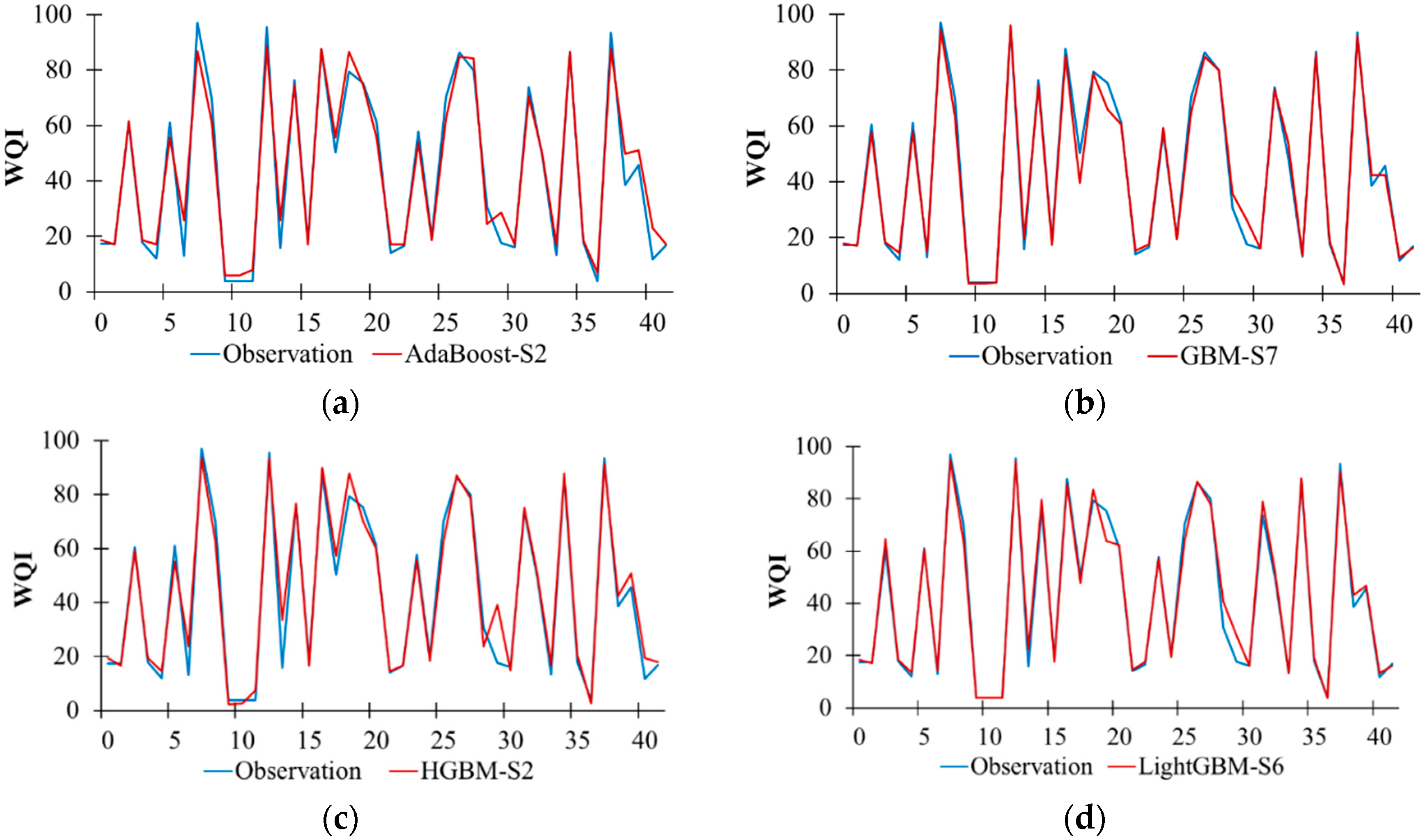
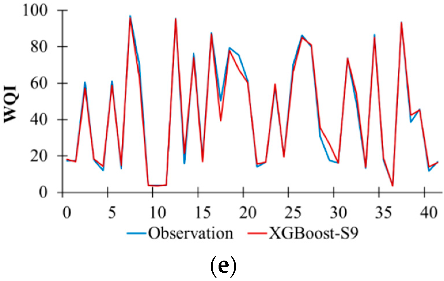
	R2	0.773	0.965	0.962	0.964	0.977	0.961	0.982	0.942	0.937	0.895

exhibits the model performance of the boosting-based algorithms during the testing process. Results showed that AdaBoost-S2 (R² = 0.973 and RMSE = 0.175) had the highest performance in predicting WQI among the AdaBoost models, GBM-S7 (R² = 0.989 and RMSE = 0.108) had the highest performance among the GBM models, HGBM-S2 (R² = 0.967 and RMSE = 0.183) had the highest performance among the GBM models, LightGBM-S6 (R² = 0.986 and RMSE = 0.119) had the highest performance among the LightGBM models, and XGBoost-S9 (R² = 0.989 and RMSE = 0.107) had the highest performance among the XGBoost models under the S1–S10 scenarios. Additionally, the comparison plots of the measured WQI values with the WQI values predicted by AdaBoost-S2, GBM-S7, HGBM-S2, LightGBM-S6, and XGBoost-S9 in the testing period are shown in Figure 2. Generally, these models replicated very well the measured WQI during the testing period. However, there are small discrepancies between the measured and predicted WQI high or low values (especially those of AdaBoost-S2 and HGBM-S2). On the whole, the comparison between the boosting-based models under the S1–S10 scenarios demonstrates the XGBoost-S9 model as the best performance model.

4.2. Performance Evaluation of Decision Tree-Based Models

Table 4 also presents the model performance of the decision tree-based algorithms during the testing process. The results indicated that DT-S5 (R² = 0.979 and RMSE = 0.147), ExT-S5 (R² = 0.985 and RMSE = 0.126), and RF-S5 (R² = 0.986 and RMSE = 0.121) had the highest performance in predicting WQI among the DT models, ExT models, and RF models under the S1–S10 scenarios, respectively. Figure 3 displays the comparisons between the predicted and measured WQI for the DT-S5, ExT-S5, and RF-S5 models during the testing period. In general, all three models reproduced well the measured WQI and small differences between the measured and predicted WQI high or low values can be seen. Regarding the model performance of the decision tree-based models, RF-S5 had the highest accurate prediction.

4.3. Performance Evaluation of ANN-Based Models

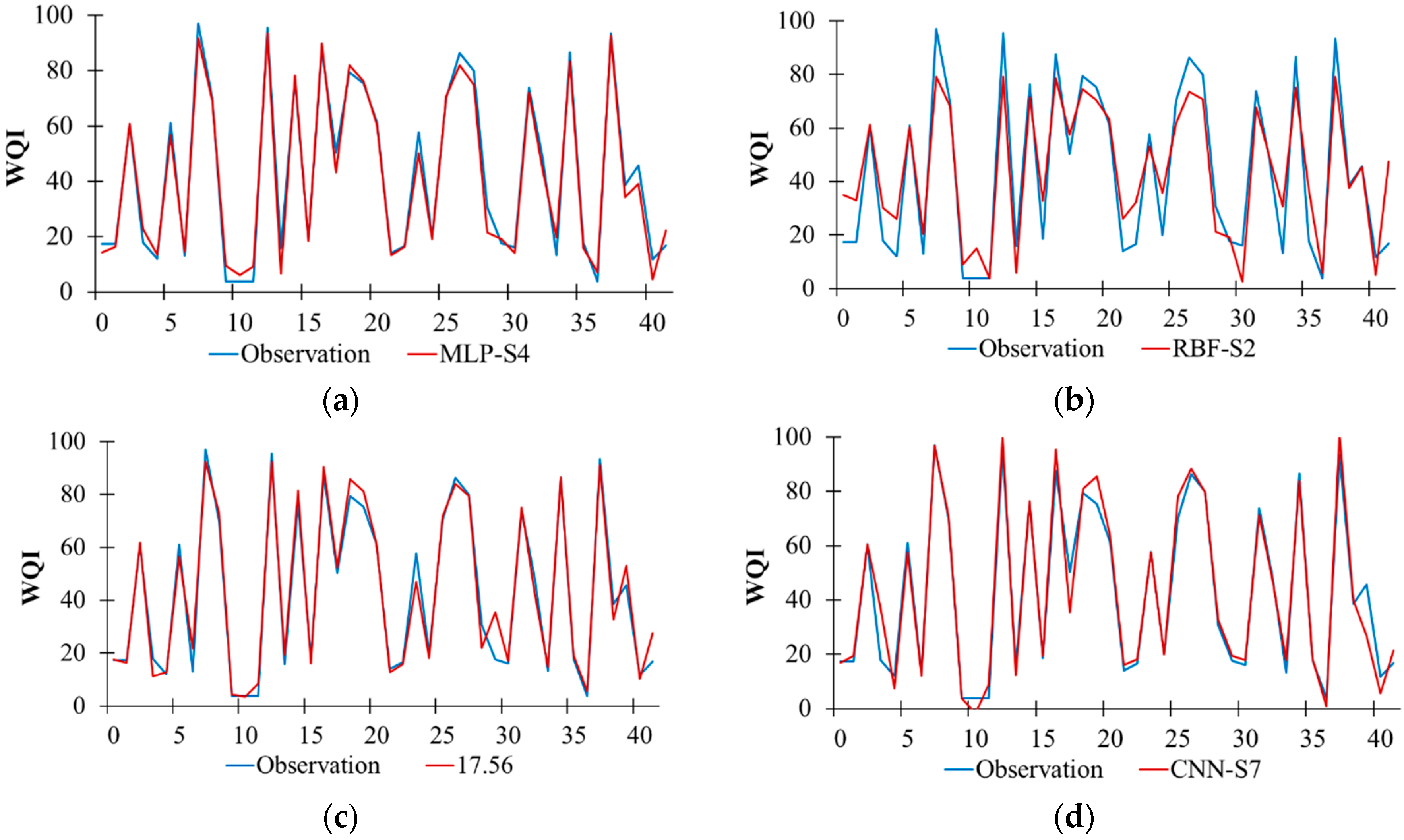
According to the model performance of the ANN-based algorithms during the testing period (Table 4), MLP-S4 (R² = 0.984 and RMSE = 0.132), RBF-S2 (R² = 0.887 and RMSE = 0.360), DFNN-S2 (R² = 0.973 and RMSE = 0.162), and CNN-S7 (R² = 0.982 and RMSE = 0.139) are the best models for predicting WQI among the MLP models, RBF models, DFNN models, and CNN models under the S1–S10 scenarios, respectively. Figure 4 illustrates the comparisons between the predicted and measured WQI for the MLP-S4, RBF-S2, DFNN-S2, and CNN-S7 models during the testing period. Generally, these four models reproduced well the measured WQI during the testing period. Moreover, small differences between the measured and predicted WQI high or low values can be observed for most models, except for RBF-S2, which show a considerable discrepancy. Regarding the model performance of the ANN-based models, MLP-S4 had the highest accurate prediction (R² = 0.984 and RMSE = 0.132).

4.4. Discussion

A comparison of twelve ML models, including five boosting-based algorithms (Adaboost, GBM, HGBM, LightGBM, and XGBoost), three decision tree-based algorithms (DT, ExT, and RF), and four ANN-based algorithms (MLP, RBF, DFNN, and CNN), was conducted to evaluate their performance in predicting the WQI based on the model efficiency statistics. Based on the model performance of the twelve ML models, our findings indicate that all ML models could predict the WQI well for this study area, but the best scenarios of input variables to the ML models are different. This can be explained by the fact that each ML algorithm will respond in a different way to different input variables and data patterns [31]. As reported by Morton and Henderson [32] and Yang and Moyer [33], water quality data are characterized by a nonlinear distribution. In general, Adaboost, HGBM, RBF, and DFNN achieved good results under the S2 scenario of the input variables; DT, ExT, and RF achieved good results under the S5 scenario; and GBM and CNN achieved good results under the S7 scenario. In addition, MLP, LightGBM, and XGBoost performed well in Scenarios S4, S6, and S9, respectively. These findings indicate that most accurate prediction is dependent on the ML model parameters for the given scenario of input variables, which is consistent with results of Hussain and Khan [31].

After comparison of all twelve ML models, it indicated that the XGBoost model outperforms other ML models in the study area. In comparison with other studies, DFNN performs better than XGBoost, MLP, and RF in the Mahanadi River Basin in India [5]. Asadollah et al. [4] indicated that ExT is superior to DT and support vector regression (SVR) in the Lam Tsuen River in Hong Kong. Moreover, DT performs better as compared to the MLP model in the Rawal Dam lake in Pakistan [14]. In general, different ML algorithms will give different performance when applied to different regions. Therefore, exploring and developing a generalized ML model for applications of water quality assessment is an ongoing struggle.

As stated in previous studies, an important gap is a lack of considering cross influences between the explanatory variables, namely, the cross-correlation between land-use classes and the cross-correlation between climate conditions in influencing river water quality [34,35,36]. Land-use change and climate change affect hydrological components, and consequently river discharge and pollutant transport [21]. Therefore, it is essential to take into account land-use and climate changes, which may improve the accuracy of the ML models.

5. Conclusions

This research work was conducted to investigate the capability of twelve ML models, namely, five boosting-based algorithms (Adaboost, GBM, HGBM, LightGBM, XGBoost), three decision tree-based algorithms (DT, ExT, and R)), and four ANN-based algorithms (MLP, RBF, DFNN, and CNN), in predicting the WQI. The four WQ monitoring stations alongside the La Buong River were considered as a case study. Two model efficiency statistics (i.e., R² and RMSE) were chosen for performance comparison of the different ML models. XGBoost achieved an R² of 0.989 and RMSE of 0.107 in the testing process, thus being the most appropriate ML algorithm in the study area. It was followed by GBM, LightGBM, RF, ExT, MLP, CNN, DT, DFNN, AdaBoost, HGBM, and RBF. Generally, our findings strengthen the argument that ML models, particularly XGBoost, can be utilized for predicting the WQI with a high degree of accuracy, which will further improve water quality management.

References

- Nouraki, A.; Alavi, M.; Golabi, M.; Albaji, M. Prediction of water quality parameters using machine learning models: A case study of the Karun River, Iran. Environ. Sci. Pollut. Res. 2021, 28, 57060–57072. [Google Scholar] [CrossRef] [PubMed]
- Ambade, B.; Sethi, S.S. Health Risk Assessment and Characterization of Polycyclic Aromatic Hydrocarbon from the Hydrosphere. J. Hazard. Toxic Radioact. Waste 2021, 25, 05020008. [Google Scholar] [CrossRef]
- Ambade, B.; Sethi, S.S.; Giri, B.; Biswas, J.K.; Bauddh, K. Characterization, Behavior, and Risk Assessment of Polycyclic Aromatic Hydrocarbons (PAHs) in the Estuary Sediments. Bull. Environ. Contam. Toxicol. 2022, 108, 243–252. [Google Scholar] [CrossRef] [PubMed]
- Asadollah, S.B.H.S.; Sharafati, A.; Motta, D.; Yaseen, Z.M. River water quality index prediction and uncertainty analysis: A comparative study of machine learning models. J. Environ. Chem. Eng. 2021, 9, 104599. [Google Scholar] [CrossRef]
- Singha, S.; Pasupuleti, S.; Singha, S.S.; Singh, R.; Kumar, S. Prediction of groundwater quality using efficient machine learning technique. Chemosphere 2021, 276, 130265. [Google Scholar] [CrossRef]
- Brown, R.M.; McClelland, N.I.; Deininger, R.A.; Tozer, R.G. A water quality index-do we dare. Water Sew. Work. 1970, 117, 339–343. [Google Scholar]
- Bui, D.T.; Khosravi, K.; Tiefenbacher, J.; Nguyen, H.; Kazakis, N. Improving prediction of water quality indices using novel hybrid machine-learning algorithms. Sci. Total Environ. 2020, 721, 137612. [Google Scholar] [CrossRef]
- Tiyasha; Tung, T.M.; Yaseen, Z.M. A survey on river water quality modelling using artificial intelligence models: 2000–2020. J. Hydrol. 2020, 585, 124670. [Google Scholar] [CrossRef]
- Nearing, G.S.; Kratzert, F.; Sampson, A.K.; Pelissier, C.S.; Klotz, D.; Frame, J.M.; Prieto, C.; Gupta, H.V. What Role does Hydrological Science Play in the Age of Machine Learning? Water Resour. Res. 2021, 57, e2020WR028091. [Google Scholar] [CrossRef]
- El Bilali, A.; Taleb, A.; Brouziyne, Y. Groundwater quality forecasting using machine learning algorithms for irrigation purposes. Agric. Water Manag. 2021, 245, 106625. [Google Scholar] [CrossRef]
- Nayan, A.-A.; Kibria, M.G.; Rahman, M.O.; Saha, J. River Water Quality Analysis and Prediction Using GBM. In Proceedings of the 2020 2nd International Conference on Advanced Information and Communication Technology (ICAICT), Dhaka, Bangladesh, 28–29 November 2020; IEEE: New York, NY, USA, 2020; pp. 219–224. [Google Scholar]
- Bedi, S.; Samal, A.; Ray, C.; Snow, D. Comparative evaluation of machine learning models for groundwater quality assessment. Environ. Monit. Assess. 2020, 192, 776. [Google Scholar] [CrossRef] [PubMed]
- Radhakrishnan, N.; Pillai, A.S. Comparison of Water Quality Classification Models using Machine Learning. In Proceedings of the 2020 5th International Conference on Communication and Electronics Systems (ICCES), Coimbatore, India, 10–12 June 2020; IEEE: New York, NY, USA, 2020; pp. 1183–1188. [Google Scholar]
- Ahmed, M.; Mumtaz, R.; Hassan Zaidi, S.M. Analysis of water quality indices and machine learning techniques for rating water pollution: A case study of Rawal Dam, Pakistan. Water Supply 2021, 21, 3225–3250. [Google Scholar] [CrossRef]
- Naloufi, M.; Lucas, F.S.; Souihi, S.; Servais, P.; Janne, A.; Wanderley Matos De Abreu, T. Evaluating the Performance of Machine Learning Approaches to Predict the Microbial Quality of Surface Waters and to Optimize the Sampling Effort. Water 2021, 13, 2457. [Google Scholar] [CrossRef]
- Gazzaz, N.M.; Yusoff, M.K.; Aris, A.Z.; Juahir, H.; Ramli, M.F. Artificial neural network modeling of the water quality index for Kinta River (Malaysia) using water quality variables as predictors. Mar. Pollut. Bull. 2012, 64, 2409–2420. [Google Scholar] [CrossRef] [PubMed]
- Hameed, M.; Sharqi, S.S.; Yaseen, Z.M.; Afan, H.A.; Hussain, A.; Elshafie, A. Application of artificial intelligence (AI) techniques in water quality index prediction: A case study in tropical region, Malaysia. Neural Comput. Appl. 2017, 28, 893–905. [Google Scholar] [CrossRef]
- Bowes, B.D.; Wang, C.; Ercan, M.B.; Culver, T.B.; Beling, P.A.; Goodall, J.L. Reinforcement learning-based real-time control of coastal urban stormwater systems to mitigate flooding and improve water quality. Environ. Sci. Water Res. Technol. 2022. [Google Scholar] [CrossRef]
- Prasad, D.V.V.; Venkataramana, L.Y.; Kumar, P.S.; Prasannamedha, G.; Harshana, S.; Srividya, S.J.; Harrinei, K.; Indraganti, S. Analysis and prediction of water quality using deep learning and auto deep learning techniques. Sci. Total Environ. 2022, 821, 153311. [Google Scholar] [CrossRef]
- MONRE. Decision No. 879/QD-TCMT on the Guidelines for Calculating Water Quality Index (WQI); Ministry of Natural Resources and Environment: Hanoi, Vietnam, 2011.
- Khoi, D.N.; Nguyen, V.; Sam, T.T.; Nhi, P. Evaluation on Effects of Climate and Land-Use Changes on Streamflow and Water Quality in the La Buong River Basin, Southern Vietnam. Sustainability 2019, 11, 7221. [Google Scholar] [CrossRef] [Green Version]
- Grayman, W.M.; Day, H.J.; Luken, R. Regional water quality management for the Dong Nai River Basin, Vietnam. Water Sci. Technol. 2003, 48, 17–23. [Google Scholar] [CrossRef]
- Najah Ahmed, A.; Binti Othman, F.; Abdulmohsin Afan, H.; Khaleel Ibrahim, R.; Ming Fai, C.; Shabbir Hossain, M.; Ehteram, M.; Elshafie, A. Machine learning methods for better water quality prediction. J. Hydrol. 2019, 578, 124084. [Google Scholar] [CrossRef]
- Zhou, Z.-H. Ensemble Methods: Foundations and Algorithms, 1st ed.; Chapman and Hall: Boca Raton, FL, USA, 2012. [Google Scholar]
- Schapire, R.E. The Boosting Approach to Machine Learning: An Overview. In Nonlinear estimation and classification; Springer: Berlin/Heidelberg, Germany, 2003; pp. 149–171. [Google Scholar]
- Wu, T.; Zhang, W.; Jiao, X.; Guo, W.; Hamoud, Y.A. Comparison of five Boosting-based models for estimating daily reference evapotranspiration with limited meteorological variables. PLoS ONE 2020, 15, e0235324. [Google Scholar] [CrossRef] [PubMed]
- Geetha, A.; Nasira, G.M. Data mining for meteorological applications: Decision trees for modeling rainfall prediction. In Proceedings of the 2014 IEEE International Conference on Computational Intelligence and Computing Research, Coimbatore, India, 18–20 December 2014; IEEE: New York, NY, USA, 2014; pp. 1–4. [Google Scholar]
- Ahmad, M.W.; Reynolds, J.; Rezgui, Y. Predictive modelling for solar thermal energy systems: A comparison of support vector regression, random forest, extra trees and regression trees. J. Clean. Prod. 2018, 203, 810–821. [Google Scholar] [CrossRef]
- Tahmasebi, P.; Kamrava, S.; Bai, T.; Sahimi, M. Machine learning in geo- and environmental sciences: From small to large scale. Adv. Water Resour. 2020, 142, 103619. [Google Scholar] [CrossRef]
- Krause, P.; Boyle, D.P.; Bäse, F. Comparison of different efficiency criteria for hydrological model assessment. Adv. Geosci. 2005, 5, 89–97. [Google Scholar] [CrossRef] [Green Version]
- Hussain, D.; Khan, A.A. Machine learning techniques for monthly river flow forecasting of Hunza River, Pakistan. Earth Sci. Informatics 2020, 13, 939–949. [Google Scholar] [CrossRef]
- Morton, R.; Henderson, B.L. Estimation of nonlinear trends in water quality: An improved approach using generalized additive models. Water Resour. Res. 2008, 44, W07420. [Google Scholar] [CrossRef]
- Yang, G.; Moyer, D.L. Estimation of nonlinear water-quality trends in high-frequency monitoring data. Sci. Total Environ. 2020, 715, 136686. [Google Scholar] [CrossRef]
- Kouadri, S.; Elbeltagi, A.; Islam, A.R.M.T.; Kateb, S. Performance of machine learning methods in predicting water quality index based on irregular data set: Application on Illizi region (Algerian southeast). Appl. Water Sci. 2021, 11, 190. [Google Scholar] [CrossRef]
- Kung, C.-C.; Wu, T. Influence of water allocation on bioenergy production under climate change: A stochastic mathematical programming approach. Energy 2021, 231, 120955. [Google Scholar] [CrossRef]
- Kung, C.-C.; Mu, J.E. Prospect of China’s renewable energy development from pyrolysis and biochar applications under climate change. Renew. Sustain. Energy Rev. 2019, 114, 109343. [Google Scholar] [CrossRef]
Figure 1.
The La Buong River and location of the WQ monitoring stations.
Figure 2.
Temporal variation in the observed and predicted WQI values for the best performance models using boosting-based algorithms during the testing period. (a) AdaBoost-S2. (b) GBM-S7. (c) HGBM-S2. (d) LightGBM-S6. (e) XGBoost-S9.
Figure 3.
Temporal variation in the observed and predicted WQI values for the best performance models using decision tree-based algorithms during the testing period. (a) DT-S5. (b) ExT-S5. (c) RF-S5.
Figure 4.
Temporal variation in the observed and predicted WQI values for the best performance models using ANN-based algorithms during the testing period. (a) MLP-S4. (b) RBF-S2. (c) DFNN-S2. (d) CNN-S7.