Measurement of Agricultural Water and Land Resource System Vulnerability with Random Forest Model Implied by the Seagull Optimization Algorithm

Abstract

To evaluate the state of an agricultural development more comprehensively, a vulnerability assessment is introduced into agricultural water and land resources system, and it is expected that the vulnerability assessment can provide a basis for improving system structure and function and realizing sustainable development. In the study, 27 evaluation indicators are selected from the agricultural water and land resources system (AWLRS), socio-economic system and ecological structure system to construct the evaluation index system for agricultural water and land resource system vulnerability (AWLRSV). Seagull optimization algorithm (SOA) is used to calibrate the parameters of the random forest (RF) model. SOA-RF model is applied to measure the AWLRSV of Heilongjiang Province in China. The results show that the SOA-RF model has higher accuracy and stronger stability than the traditional RF model and DA-RF model. The value of AWLRSV in Heilongjiang Province presents a downward–upward–downward trend from 2008 to 2018. The vulnerability levels are mainly level II and III, and level III is mainly distributed northwest and southeast of Heilongjiang Province. The novelty of this paper is to regard the agricultural water and land resources system as a compound system, put forward the vulnerability assessment framework. The findings may provide reference for regional sustainable development from a new research perspective.

1. Introduction

Agriculture is the basis of socio-economic development and the maintenance of ecological environment [1]. As the core resources of agricultural production, the utilization of agricultural water and land resources directly influences the degree of regional development. As a criterion to measure the degree of regional development, vulnerability research is becoming more and more important in the fields of regional sustainable development, global climate change development, and system development trends [2]. The area of black soil farmland in Heilongjiang Province is 12.08 million hm², accounting for about 44% of the black soil area in northeast China, which is one of the three black soil zones in the world [3]. Due to unreasonable farming practices, extensive use of chemical fertilizers, and excessive reclamation, soil quality has declined and food production has been severely restricted. Therefore, it is of great importance to evaluate the AWLRSV in Heilongjiang Province for rational planning of agricultural resources, and it can provide a new path for the sustainable development of countries and regions.

The concept of vulnerability, which originated in the field of natural hazard-related disasters, refers to the ability to deal with disruption that is below a certain critical threshold; it indicates that the area is vulnerable [4]. With the depletion of resources and the deterioration of the environment, vulnerability assessment has been widely addressed by scholars from diverse perspectives. Turner et al. revised and expanded the basic design of vulnerability analysis, and proposed the vulnerability assessment framework for a human–environment coupled system [5]. Kerzabi et al. used remote sensing and GIS to measure groundwater vulnerability, and the results showed the vulnerability map can provide a basis for delineating the areas for groundwater protection and land management [6]. Shen et al. considered the influence of four stressors on the vulnerability of urban ecosystem, and then evaluated its vulnerability, and the results can provide reference for decision makers to take measures to protect human health and environmental quality [7]. Men et al. developed an index of water resources system vulnerability by using the pressure–state–response model, and evaluated the water resources vulnerability based on the attribute recognition model. The results showed it was necessary to take corresponding measures to protect the water resources of the Heihe River Basin [8]. According to previous studies, vulnerability has been widely used in the fields of disaster management, ecology, geosciences, engineering, land use, sustainable science, etc. However, an in-depth view of the vulnerability research on the AWLRS is still very weak. Water resources and cultivated land resources are the basic components of agricultural development. Whether the utilization of water resources is reasonable or not will directly influence the production efficiency of land resources, and the quantity and quality of cultivated land resources also directly restrict the utilization of water resources, and they are interrelated, permeate and restrict each other [1]. Respective study of the system of water and land resources only separately will hinder the full play of the overall efficiency, and easily lead to the overload operation of the system. Therefore, it is necessary to evaluate the vulnerability of water and land resources system as a whole.

With regard to the in-depth study of vulnerability, lots of assessment tools have been developed. Zhang et al. used the index evaluation method to measure the ecosystem vulnerability of wetlands, and the results showed that the wetland ecosystem is moderately vulnerable in the Yellow River Delta from 2005 to 2014 [9]. Chen et al. studied the social-ecosystem vulnerability and analyzed the spatial differentiation characteristics and evolution trend of vulnerability in Yulin City from 2000 to 2011 by using RS and GIS spatial technology, and discussed the internal reasons for the spatio-temporal evolution of vulnerability [10]. Zhi used a fuzzy comprehensive method to build the vulnerability assessment model of water resources and establish corresponding evaluation criteria by taking the administrative district of Guangdong as research area [11]. The above methods provide a type of research method for vulnerability assessment, but there are still some shortcomings. (1) The index evaluation method ignores the internal relationship of indicators and has strong subjectivity, and so it is difficult to verify the results of vulnerability evaluation. (2) The method based on GIS and RS is limited by the imperfect theoretical system of vulnerability, and the development is slow. (3) The selection of the reference system of the fuzzy comprehensive method is subjective, and the evaluation results can only reflect the relative value. Therefore, when choosing the vulnerability quantification method, we should avoid the above problems and choose a model with a better comprehensive performance for evaluation purposes. Within the context of the wide application of artificial intelligence, the machine learning method has been recognized as useful. Been regarded as one of the best machine learning methods, random forest (RF) has excellent tolerance to noise, high prediction accuracy, strong data mining capabilities, and is good at dealing with multi-feature data [12,13,14]. Therefore, we choose the RF model to measure the AWLRSV. In the RF, the setting and selection of the number of subset size of attribute characteristics (mtry) and decision trees (ntree) is an important problem that affects the performance of the model [15]. SOA is proposed in 2018 as a new swarm intelligence optimization algorithm, and a previous study revealed that SOA is very competitive compared with nine well-known optimization algorithms [16]. Therefore, this paper introduces SOA to optimize RF to solve the uncertainty of optimal parameter (i.e., ntree and mtry) selection in traditional RF model.

The purpose of this paper is to introduce vulnerability assessment into agricultural water and land resources system as a basis for evaluating the development status of agricultural system, use SOA to improve the RF model, and evaluate the performance of the SOA-RF model. Specific objectives are as follows:

• Construct the index evaluation system based on the multi-system, and evaluate the AWLRSV based on SOA-RF model;
• Analyze the stability and accuracy of the SOA-RF model;
• Explore the spatio-temporal variation characteristics of AWLRSV in Heilongjiang Province.

2. Materials and Methods

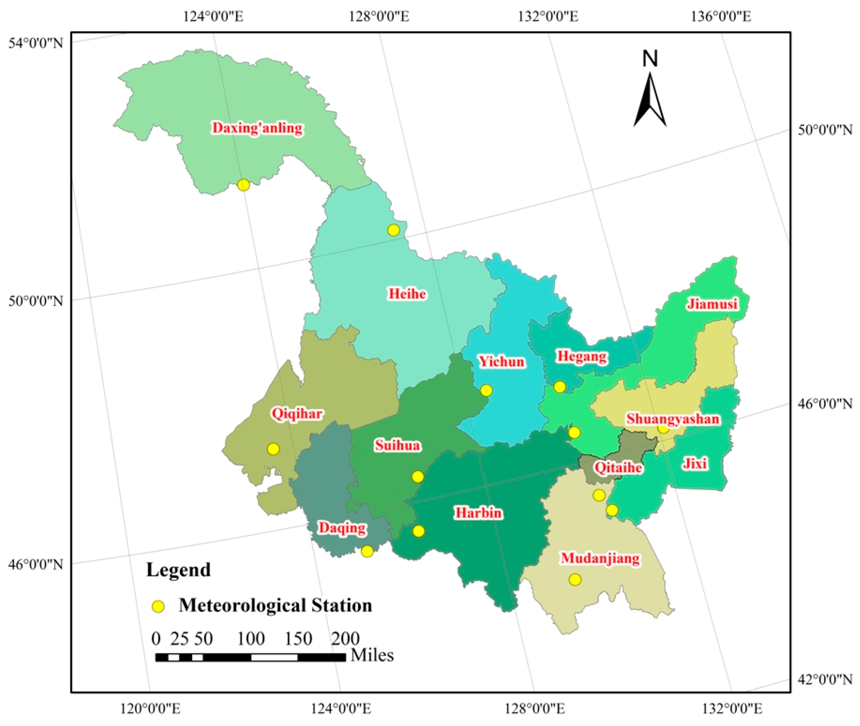
2.1. Study Area

Heilongjiang Province a major province of grain production in China, which is located in the north of Northeast China (Figure 1). The land is rich and fertile, the agricultural land area accounts for 88% of the total land area, and has two major commodity grain bases (Songnen Plain and Sanjiang Plain). The precipitation has obvious monsoon characteristics. The total amount of water resources is more than 74 billion m³, and the annual precipitation in each region is between 400~600 mm. However, the amount of water resources per unit area of cultivated land is only 1/3 of the national average level, the spatio-temporal distribution of water resources is uneven, widespread drought and water shortage are common, which seriously limits agricultural production capacity.

2.2. Data Sources

Limited by the availability of data, the data during the study were updated to 2018. Therefore, the period from 2008 to 2018 is selected as the research period in this paper. The study area includes 13 cities in the Heilongjiang Province as well as the respective rural areas. The data of water and land resources, social economy and other indicators were obtained from Heilongjiang Water Conservancy Statistical Bulletin, Heilongjiang Water Resources Bulletin and Heilongjiang Statistical Year Book. The land area was obtained by remote sensing monitoring, the ecological structure indexes such as habitat quality index, forest and grass coverage, water area ratio, cultivated land and construction land area ratio were obtained by calculation. The meteorological parameters such as temperature, precipitation, sunshine hours, and relative humidity were obtained from China Meteorological data Network (http://data.cma.cn (accessed on 1 May 2021)), and the meteorological stations were shown in Figure 1.

2.3. Random Forest Model

Random forest (RF) is an integrated algorithm composed of decision trees. In the integrated algorithm, several independent decision trees are constructed by bagging, and the results are determined according to the average or majority voting principle, so as to reduce the risk of data over-fitting [17,18]. In the process of forest generation, the number of mtry and ntree and are two important parameters which directly affects the performance of RF model [19]. In traditional RF model, the value of ntree and mtry are based on experience and have a certain degree of uncertainty.

The forest is composed of multiple decision trees $\left\{h\left({x,\theta }_j\right), m=1,2,3,\dots N\right\}$. The algorithm flow is as follows [15,18]:

Using the bootstrap method to repeat random extraction of original data to generate j sets ${\theta }_1{,\theta }_2$,…,${\theta }_j$, and the corresponding j decision trees.

If the feature is M-dimensional, specify the constant m, randomly select m sub-feature sets from M-dimensional features, and obtain the best segmentation according to the above way of establishing the decision tree.

Each decision tree grows without pruning and grows freely until it can no longer split.

Generating j decision trees to constitute a random forest, and determine the best decision tree by voting.

Taking the average value of j decision trees $h\left({x,\theta }_j\right)$ as the final result.

2.4. Seagull Optimization Algorithm

SOA is a bionic intelligent optimization algorithm, and its optimization idea comes from the migrating and attacking behaviors [16].

2.4.1. Migrating Behavior

During migrating, the algorithm simulates how a flock of seagulls moves from one location to another. The process contains three steps:

Avoiding collision: To avoid collisions between adjacent seagulls, an additional variable A is introduced to update the position.

$${\overrightarrow{C}}_s=A\times {\overrightarrow{P}}_s(t)$$

(1)

where ${\overrightarrow{C}}_s$ is the position where the search agent does not collide with other search agents, t is the current iteration, ${\overrightarrow{P}}_s$ is the current position of search agent, and A is the movement behavior of search agent.

$$A=f_c-(t\times (f_c/\mathrm{M}a{x}_{\mathrm{iteration}})),t=0,1,\cdots ,\mathrm{M}a{x}_{\mathrm{iteration}}$$

(2)

where f_c is introduced to control the frequency of employing variable A which is linearly decreased from f_c to 0.

Movement towards the direction of the best neighbor: The searchers are moving towards the direction of the best neighbor after avoiding collision.

$${\overrightarrow{M}}_s=B\times ({\overrightarrow{P}}_{bs}(t)-{\overrightarrow{P}}_s(t))$$

(3)

where ${\overrightarrow{M}}_s$ is the positions of search agent ${\overrightarrow{P}}_s$ towards the best fit search agent ${\overrightarrow{P}}_{bs}$. The behavior of B is randomized which is responsible for proper balancing between exploration and exploitation. B is calculated as:

$$B=2\times A^2\times r_d$$

(4)

where r_d is a random number in the range of [0, 1].

Stay close to the best searcher agent: the search agent can update its position with respect to the best search agent.

$${\overrightarrow{D}}_s=\left|{\overrightarrow{C}}_s+{\overrightarrow{M}}_s\right|$$

(5)

where ${\overrightarrow{D}}_s$ represents the distance between the search agent and the best fit search agent.

2.4.2. Attacking Behavior

While attacking the prey, the spiral movement behavior occurs in the air.

This behavior is described as follows.

$$x=r\times \cos (\beta )$$

(6)

$$y=r\times \sin (\beta )$$

(7)

$$z=r\times \beta$$

(8)

$$r=u\times e^{\beta v}$$

(9)

where r is the radius of each turn of the spiral, k is a random number in range [0 ≤ k ≤ 2π]. u and v are constants to define the spiral shape, and e is the base of the natural logarithm.

$${\overrightarrow{P}}_s(t)=({\overrightarrow{D}}_s\times x\times y\times z)+{\overrightarrow{P}}_{bs}(t)$$

(10)

where ${\overrightarrow{P}}_s(t)$ saves the best solution and updates the position of other search agents.

2.5. SOA-RF Model

In the traditional RF model, the setting and selection of the number of subset size of attribute characteristics (mtry) and decision trees (ntree) is an important problem that affects the performance of the model [15]. In order to solve the problem of uncertain parameter selection in traditional RF model, SOA-RF model is proposed for optimizing mtry and ntree. First, select the mtry and ntree of the RF for the seagull individual. In order to obtain the optimal value of mtry and ntree, the SOA-RF model is constructed by taking the root mean square error (RMSE) as objective function. The detailed process is as follows.

Step 1: Build the training sets and test sets needed for the simulation.

Step 2: Initialize setting for parameters, including the position of the seagull individual (ntree and mtry), the maximum iterations i, the number of seagull populations dim, and the lower and upper bound of the optimal value search range [lb, ub].

Step 3: Bring the current seagull individual into the RF.

Step 4: Determine the fitness of current seagull individual using RMSE, as follows:

$$RMSE=\sqrt{\frac{1}{c}{\displaystyle \sum _{i=1}^c{(a_i-b_i)}^2}}$$

(11)

where c is the number of training sets, b_i is the predicted value, and a_i is the true value.

Step 5: The iteration is ended when the number of iterations reaches expected maximum or conforms to the optimal value of the objective function. Otherwise, return to the Step 3.

Step 6: Output the optimal parameters (mtry and ntree) in SOA-RF model.

The SOA-RF model process is shown in Figure 2.

2.6. The Verification of Model Performance

2.6.1. Accuracy Analysis

The coincidence degree between the predicted value and the real value is expressed by the mean absolute percentage error (MAPE). The MAPE is calculated as follows:

$$MAPE=\frac{100\%}{n}{{\displaystyle \sum }}_{i=1}^n\left|\frac{{\widehat{y}}_i-y_i}{y}\right|$$

(12)

where n is the number of training sets; $y_i$ and ${\widehat{y}}_i$ are predicted value and real value, respectively. MAPE varies between 0 and 1, the smaller the MAPE is, the higher the coincidence degree is and the higher the accuracy of the model is.

The fitting degree between the predicted value and the real value is expressed by the coefficient of determination ($R^2$), and it is calculated as follows.

$$R^2=1-\frac{{{\displaystyle \sum }}_i{\left({\widehat{y}}_i-y_i\right)}^2}{{{\displaystyle \sum }}_i{\left(\overline{y}-y_i\right)}^2}$$

(13)

where $y_i$ and ${\widehat{y}}_i$ are predicted value and real value, respectively, $\overline{y}$ is the mean value of predicted value. $R^2$ varies between 0 and 1, the larger the $R^2$ is, the higher the fitting degree is, and the better the model performance is.

2.6.2. Stability Analysis

The stability of an evaluation method depends on the rationality of applying the evaluation method to the ranking of evaluation results. In order to analyze the stability of the evaluation method, the theories of serial number summation and Spearman correlation coefficient are introduced to compare the performance of different methods.

According to the sequence number summation theory, the reasonable sorting result is the sorting result of the sequence number summation of each method [20]. First of all, the evaluation objects are evaluated by different methods, and the sequence numbers of each evaluation results are added and reordered. Then, the Spearman correlation coefficients are calculated. The Spearman correlation coefficient is calculated as follows:

$$R=1-\frac{6\times {\displaystyle \sum D_i^2}}{n(n^2-1)}$$

(14)

where R is the correlation coefficient, n is the number of regions, $D_i$ represents the difference value between the ordering result and the reasonable ordering result. R varies between 0 and 1, and the larger the R is, the more stable the model is.

3. Results

3.1. The Establishment of Evaluation Index System for AWLRSV

According to the connotation of vulnerability and multi-system evaluation index system, 27 evaluation indicators were selected from the water and land resources system, socio-economic system and ecological structure system to construct the AWLRSV evaluation index system, as shown in

Table 1. AWLRSV evaluation index system.

System	Index	Type	Indicator Calculation
Water and land resources	Matching coefficient of agricultural water and land resources (C1)	+	Generalized water resources/cultivated area, as shown in the reference [21]
	Reclamation rate (C2)	+	Cultivated area/Total land area
	Precipitation (C3)	−	Get it from Heilongjiang Water Resources Bulletin
	Agricultural water quota (C4)	+	Agricultural water consumption/ Agricultural GDP
	Agricultural irrigation rate (C5)	+	Irrigation area/cultivated land area
	Planting proportion of crops with high water consumption (C6)	+	Rice area/Crop area
	Proportion of agricultural water use (C7)	+	Agricultural water consumption/Total water consumption
	Agricultural water consumption per unit cultivated land (C8)	+	Agricultural water consumption/Cultivated area
	Grain yield per unit water (C9)	+	Grain yield/Agricultural water consumption
	Grain yield per unit cultivated area (C10)	+	Grain yield/Cultivated area
	Drainage area (C11)	−	Obtain it from Heilongjiang Water Conservancy Statistical Bulletin
	Water and land loss control area (C12)	−	Obtain it from Heilongjiang Water Conservancy Statistical Bulletin
	Fertilizer application per unit area (C13)	+	Fertilizer use/cultivated land area
	Total reservoir capacity (C14)	−	Obtain it from Heilongjiang Water Conservancy Statistical Bulletin
Socio-economic	Total investment in water conservancy (C15)	−	Obtain it from Heilongjiang Water Conservancy Statistical Bulletin
	Urbanization rate (C16)	−	Urban population/total population
	Agricultural GDP per unit cultivated land (C17)	−	Agricultural GDP/Cultivated land area
	Per capita water resources (C18)	−	Total water resources/total population
	Population density(C19)	+	Total population/Total land area
	Proportion of agricultural GDP (C20)	+	Agricultural GDP/GDP
	Per capita cultivated area (C21)	−	Cultivated land area/total population
	Degree of Agricultural Mechanization (C22)	−	Total power of agricultural machinery/Cultivated land area
Ecological structure	Habitat quality index (C23)	−	“HJ192-2015 Technical Criterion for Ecosystem Status Evaluation”
	Forest and grass coverage (C24)	−	Sum of forest and grassland area/Total land area
	Proportion of water wetland area (C25)	−	Water wetland area/Total land area
	Proportion of cultivated and construction land (C26)	+	Sum of cultivated and construction land/Total land area
	Gray water footprint (C27)	+	Dilute the maximum amount of fresh water required for each pollutant in crop production, and as shown in the reference [21]

(Note: “+” represents the positive index, “−” and represents the negative index).

.

3.2. AWLRSV Rating Criteria

In order to observe the temporal and spatial variations changes of AWLRSV in Heilongjiang Province, the evaluation time interval is set from 2008 to 2018. The mean value of indicators is used as the passing value, the maximum value of positive indicators or the minimum value of negative indicators are used as the optimal value, the minimum value of positive indicators or the maximum value of negative indicators are used as the worst value, the average value between worst and passing value are used as worse value, the average value between optimal and passing value are used as better value. The feature nodes of each evaluation index are shown in

Table 2. Feature nodes of AWLRSV evaluation index.

Evaluation Index	Worst Value	Worse Value	Passing Value	Better Value	Optimal Value
Matching coefficient of agricultural water and land resources (C1)	0	0.25	0.35	0.48	1
Reclamation rate (C2)	0	4	40	55	80
Precipitation (C3)	600	283	188	103	9
Agricultural water quota (C4)	1	470	920	1760	6328
Agricultural irrigation rate (C5)	0	9	17	30	60
Planting proportion of crops with high water consumption (C6)	0	10	20	35.8	100
Proportion of agricultural water use (C7)	0	62	80	90	100
Agricultural water consumption per unit cultivated land (C8)	0	468	1040	1573	2700
Grain yield per unit water (C9)	4	36.8	193	1280	4500
Grain yield per unit cultivated area (C10)	0	2.38	3.48	5.19	8
Drainage area (C11)	421	265	132	45	2
Water and land loss control area (C12)	1074	626	312	133	21
Fertilizer application per unit area (C13)	80	165	237	344	500
Total reservoir capacity (C14)	968,798	460,506	151,617	47,692	0
Total investment in water conservancy (C15)	661,400	136,099	68,520	28,724	1600
Urbanization rate (C16)	90	75	59	48	25
Agricultural GDP per unit cultivated land (C17)	86,000	33,039	18,175	9683	1000
Per capita water resources (C18)	62,900	16,318	5360	2072	400
Population density(C19)	6	53	90	150	200
Proportion of agricultural GDP (C20)	2	14	24	36	63
Per capita cultivated area (C21)	120	72	48	29	10
Degree of Agricultural Mechanization (C22)	8	3.5	2.4	1.4	0
Habitat quality index (C23)	170	130	106	81	60
Forest and grass coverage (C24)	100	72	46	30	10
Water wetland area ratio (C25)	13	6.2	3.5	1.4	0
Proportion of cultivated and construction land (C26)	0	16	40	55	80
Gray water footprint (C27)	0	1.6	4.8	10	18

.

The eigenvalues of the index in Table 2 are taken as the upper and lower limits of each interval, and 800 samples are randomly generated in each interval, of which 600 are training samples and the remaining 200 are test samples. The training samples and the corresponding levels are used as input source and output source to be brought into the SOA-RF model. The simulation structure model is established after training and learning, and four simulation grades (I–IV) of AWLRSV were obtained after simulation as shown in

Table 3. Simulation grades based on SOA-RF model.

Level	Little Vulnerability (I)	Less Vulnerability (II)	More Vulnerable (III)	Very Vulnerable (IV)
Interval	(1.000, 1.478]	(1.478, 2.544]	(2.544, 3.354]	(3.354, 4.000]

.

Finally, the relevant data of the research area are brought into the simulation model, and the vulnerability level of the relevant area is obtained according to Table 3.

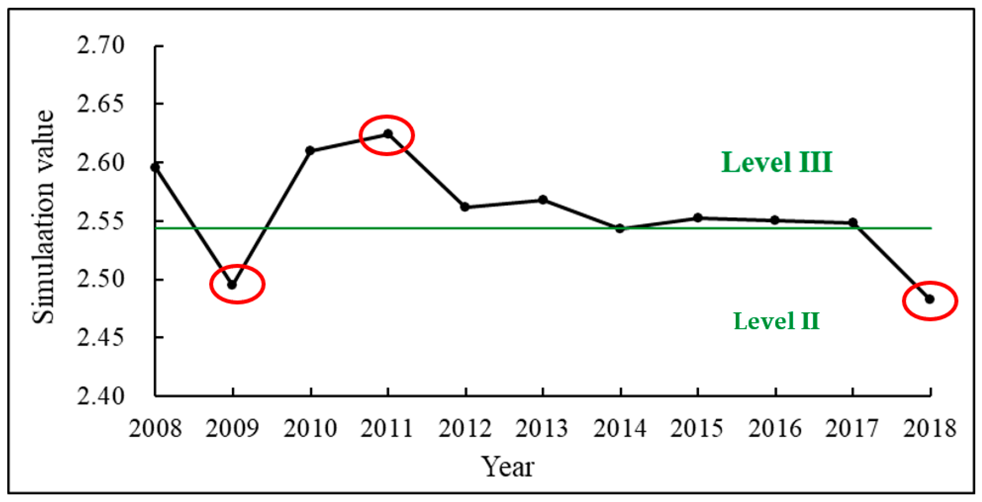
3.3. Spatio-Temporal Variation Characteristics of AWLRSV

In order to obtain the temporal variation of the AWLRSV, the relevant index data from 2008 to 2018 were brought into the SOA-RF model by taking Heilongjiang Province as the research base. The temporal variation curve was as shown in Figure 3.

From 2008 to 2018, the AWLRSV presents a downward–upward–downward trend in Heilongjiang Province. The results showed that the AWLRSV levels were mainly in II and III, and the extreme values appeared in 2009, 2011, and 2018. Three stages are divided according to the temporal variation characteristics of the AWLRSV. In the first stage (2008–2009), the level changed from level III to level II, the AWLRSV improves rapidly. According to Heilongjiang Water Resources Bulletin, the year 2009 in Heilongjiang Province is a rainy year with more precipitation, which directly affects the evaluation results of vulnerability. In the second stage (2019–2011), the AWLRSV degenerated rapidly, and the level changed from level II to level III. The main reason is that grain production and the application of chemical fertilizer increased rapidly according to data from 2009 to 2011. In the third stage (2011–2018), the level changed from level III to level II, the AWLRSV improved slowly. With the slow increase of grain output, the improvement of mechanization and the support of policies, the AWLRSV tended to get better from 2011 to 2018.

By bringing the data of evaluation index for the 13 regions in Heilongjiang Province from 2008 to 2009, 2009 to 2011, and 2011 to 2018 into the established SOA-RF model, the corresponding evaluation results and levels can be calculated as shown in

Table 4. Evaluation results and levels of AWLRSV.

Region	Evaluation Result			Evaluation Level
	2008–2009	2009–2011	2011–2018	2008–2009	2009–2011	2011–2018
Harbin	2.597	2.605	2.634	III	III	III
Qiqihar	2.526	2.691	2.738	II	III	III
Jixi	2.604	2.609	2.616	III	III	III
Hegang	2.530	2.579	2.681	II	III	III
Shuangyashan	2.584	2.519	2.471	III	II	II
Daqing	2.786	2.833	2.855	III	III	III
Yichun	2.311	2.303	2.282	II	II	II
Jiamusi	2.761	2.799	2.890	III	III	III
Qitaihe	2.705	2.778	2.755	III	III	III
Mudanjiang	2.270	2.253	2.087	II	II	II
Heihe	2.317	2.323	2.160	II	II	II
Suihua	2.979	2.977	2.912	III	III	III
Daxing’anling	2.113	2.221	2.122	II	II	II
Average	2.545	2.617	2.554	III	III	III

.

Table 4 shows that the average value of AWLRSV of 13 cities in Heilongjiang Province was 2.545 from 2008 to 2009, 2.617 from 2009 to 2011, and 2.554 from 2011 to 2018, and all the average evaluation grades were level III. Therefore, the AWLRSV is still very serious from the overall point of view of Heilongjiang Province, and continuous improvement measures should be implemented.

To illustrate the spatial distribution of AWLRSV level, the spatial distribution map of AWLRSV in Heilongjiang Province in 2008, 2009, 2011, and 2018 were plotted, as shown in Figure 4. Seen from Figure 4, the vulnerability levels are mainly level II and III, and level III is mainly distributed northwest and southeast of Heilongjiang Province.

4. Discussion

4.1. Accuracy Analysis of SOA-RF Model

RMSE is calculated based on the Formula (11), MAPE is calculated based on the Formula (12), R² is calculated based on the Formula (13), and the results are shown in

Table 5. SOA-RF model performance indicators.

Indicator Name	RMSE	R2	MAPE
RF	0.0123	0.9998	−2.1833 × 10−4
SOA-RF	0.0050	0.9999	4.1556 × 10−6
DA-RF	0.0060	0.9999	−3.3333 × 10−5

.

As shown in Table 5, the RMSE, R² and MAPE of the SOA-RF model are 0.0050, 0.9999, 4.1556 × 10⁻⁶, respectively, which indicate that the SOA-RF model has high evaluation accuracy and can be used as an evaluation method for the vulnerability of agricultural water and land resources system. Compared with other models, due to the higher optimization performance of SOA, the fitting result of SOA-RF model is more accurate and shows better fitting ability.

4.2. Stability Analysis of SOA-RF Model

In order to analyze the stability of the SOA-RF model, the reasonable order is obtained based on the theory of serial number summation as shown in

Table 6. The serial number summation and reasonable order.

	RF	DA-RF	SOA-RF	Serial Number Summation	Reasonable Order
Harbin	8	7	7	22	7
Qiqihar	6	4	5	15	5
Jixi	7	8	8	23	8
Hegang	4	6	6	16	6
Shuangyashan	9	9	9	27	9
Daqing	2	2	3	7	2
Yichun	10	10	10	30	10
Jiamusi	3	3	2	8	3
Qitaihe	5	5	4	14	4
Mudanjiang	12	13	12	37	12
Heihe	11	11	11	33	11
Suihua	1	1	1	3	1
Daxing’anling	13	12	13	38	13

, and the Spearman correlation coefficient is calculated based on Formula (14) as shown in

Table 7. Spearman correlation coefficient of each model.

Indicator Name	RF	DA-RF	SOA-RF
Spearman correlation coefficient	0.9780	0.9890	0.9945

.

As seen from Table 6 and Table 7, the Spearman correlation coefficients of RF, DA-RF, and SOA-RF are 0.9780, 0.9890, and 0.9945, which indicates that the RF model optimized by intelligent algorithm has high stability, and the SOA-RF model is more stable than others.

4.3. Analysis of Variation Characteristics of AWLRSV

As the three major forest areas in the northwest of Heilongjiang Province, the AWLRSV of Daxing’anling, Heihe, and Yichun belong to level II all the time. Mudanjiang took the lead in implementing the project of returning farmland to forest in Heilongjiang Province in 1998, so the AWLRSV of Mudanjiang also belongs to level II. Previous studies have shown that returning farmland to forest has improved the quality of regional ecological environment, and alleviated the vulnerability of regional ecological environment [22]. The AWLRSV of Shuangyashan changed from level III to level II. The main reasons for this are attaching importance to the construction of ecological civilization, paying attention to the development of agriculture, and improving the degree of agricultural mechanization and planting technology. The AWLRSV of the other areas are all level III. According to the actual local situation, each region can take measures such as paying attention to the construction of ecological environment and returning farmland to forests to alleviate vulnerability with reference to the above-mentioned regions. The evaluation results based on the SOA-RF model are in line with the actual local situation in recent years, which further shows that the SOA-RF model can be used as a new method for evaluating the AWLRSV.

It is worth noting that the AWLRSV of each region has not yet entered level I. Corresponding adjustment directions should be proposed combining the specific key driving factors.

5. Conclusions

In this paper, a new model was constructed using the SOA to optimize RF model to assess the level of AWLRSV of 13 regions in Heilongjiang Province. The results showed that the vulnerability levels are mainly level II and III, and level III is mainly distributed northwest and southeast of Heilongjiang Province. AWLRSV improved rapidly from 2008 to 2009, degenerated rapidly from 2009 to 2011, and improved slowly from 2011 to 2018. According to the evaluation results of different areas, measures such as returning farmland to forest, attaching importance to the construction of ecological civilization, paying attention to the development of agriculture and improving the degree of agricultural mechanization and planting technology can improve the level of vulnerability. Compared with the traditional RF model and DA-RF model, the SOA-RF model has higher model accuracy and stronger stability, and it can be used as an evaluation method for the vulnerability assessment of the agricultural water and land resources system.

The agricultural water and land resources system is a huge and complex system, but due to the limitations of data acquisition, resulting in the lack of some data, the selected research period is not long, and the vulnerability evolution cannot be predicted. In future, we will focus on exploring the internal mechanism of vulnerability under different spatio-temporal scales, and further reveal its functional relationship and feedback process, in order to provide a basis for regional development policies in major grain producing areas.

References

1. Ren, S.D.; Fu, Q.; Wang, K. Regional agricultural water and soil resources carrying capacity based on macro-micro scale in Sanjiang Plain. Trans. CSAE 2011, 27, 8–14. (In Chinese) [Google Scholar]
2. Yang, F.; Ma, C.; Fang, H. Research progress on vulnerability: From theoretical research to comprehensive practice. Acta Ecol. Sin. 2019, 39, 441–453. (In Chinese) [Google Scholar]
3. Li, N.N.; Zhao, Y.S.; Zhu, L.J. The Present Management Situation, Difficulties and Countermeasures of Soil and Water Loss for Black Land in Heilongjiang Province. J. Agric. Mech. Res. 2015, 37, 259–263. (In Chinese) [Google Scholar]
4. Cumming, G.S.; Barnes, G.; Perz, S.G.; Schmink, M.; Holt, T.V. An Exploratory Framework for the Empirical Measurement of Resilience. Ecosystems 2015, 8, 975–987. [Google Scholar] [CrossRef]
5. Turner, B.; Kasperson, R.E.; Matson, P.A.; Mccarthy, J.J.; Schiller, A. A framework for vulnerability analysis in sustainability science. Proc. Natl. Acad. Sci. USA 2003, 100, 8074–8079. [Google Scholar] [CrossRef] [Green Version]
6. Kerzabi, R.; Mansour, H.; Yousfi, S.; Marín, A.I.; Navarro, B.A.; Bensefia, K.E. Contribution of remote sensing and GIS to mapping groundwater vulnerability in arid zone: Case from Amour Mountains- Algerian Saharan Atlas. J. Afr. Earth Sci. 2021, 182, 104277. [Google Scholar] [CrossRef]
7. Shen, J.; Lu, H.; Zhang, Y.; Song, X.; He, L. Vulnerability assessment of urban ecosystems driven by water resources, human health and atmospheric environment. J. Hydrol. 2016, 536, 457–470. [Google Scholar] [CrossRef]
8. Men, B.; Liu, H. Water resource system vulnerability assessment of the Heihe River Basin based on pressure-state-response (PSR) model under the changing environment. Water Sci. Technol. Water Supply 2018, 18, 1956–1967. [Google Scholar] [CrossRef]
9. Zhang, X.; Wang, L.; Fu, X.; Li, H.; Xu, C. Ecological vulnerability assessment based on PSSR in Yellow River Delta. J. Clean. Prod. 2017, 167, 1106–1111. [Google Scholar] [CrossRef]
10. Chen, J.; Yang, X.J.; Yin, S.; Wu, K.S. The vulnerability evolution and simulation of the social-ecological systems in the semi-arid area based on the VSD framework. Acta Geogr. Sin. 2016, 71, 1172–1188. (In Chinese) [Google Scholar]
11. Zhi, L.S. Vulnerability Evaluation of Water Resources in Guangdong Province; Xi’an University of Technology: Xi’an, China, 2018. (In Chinese) [Google Scholar]
12. Iverson, L.R.; Prasad, A.M.; Matthews, S.; Peters, M. Estimating potential habitat for 134 eastern US tree species under six climate scenarios. For. Ecol. Manag. 2008, 254, 390–406. [Google Scholar] [CrossRef]
13. Yaseen, Z.M.; Zaher, M.; Sulaiman, S.O. An enhanced extreme learning machine model for river flow forecasting: State-of-the-art, practical applications in water resource engineering area and future research direction. J. Hydrol. 2019, 569, 387–408. [Google Scholar] [CrossRef]
14. Liu, D.; Fan, Z.R.; Fu, Q.; Li, M.; Faiz, M.A.; Ali, S.; Li, T.X.; Zhang, L.L.; Khan, M.I. Random forest regression evaluation model of regional flood disaster resilience based on the whale optimization algorithm. J. Clean. Prod. 2019, 250, 119468. [Google Scholar] [CrossRef]
15. Rodriguez-Galiano, V.F.; Ghimire, B.; Rogan, J.; Chica-Olmo, M.; Rigol-Sanchez, J.P. An assessment of the effectiveness of a random forest classifier for land-cover classification. ISPRS J. Photogramm. Remote Sens. 2012, 67, 93–104. [Google Scholar] [CrossRef]
16. Dhiman, G.; Kumar, V. Seagull optimization algorithm: Theory and its applications for large-scale industrial engineering problems. Knowl. -Based Syst. 2019, 165, 169–196. [Google Scholar] [CrossRef]
17. Breiman, L. Random forests. Mach. Learn 2001, 45, 5–32. [Google Scholar] [CrossRef] [Green Version]
18. Strobl, C.; Malley, J.; Tutz, G. An introduction to recursive partitioning: Rationale, application, and characteristics of classification and regression trees, bagging, and random forests. Psychol. Methods 2009, 14, 323–348. [Google Scholar] [CrossRef] [Green Version]
19. Li, X.; Liu, J.; Liu, D.; Fu, Q.; Khan, M.I. Measurement and analysis of regional agricultural water and soil resource composite system harmony with an improved random forest model based on a dragonfly algorithm. J. Clean. Prod. 2021, 305, 127217. [Google Scholar] [CrossRef]
20. Lv, X.P. The evaluation and improvement of the current composite index of economic returns in industrial enterprises according to the theory of the total of orders. J. Ind. Eng. Eng. Manag. 1996, 10, 61–65. (In Chinese) [Google Scholar]
21. Zhao, D.; Chen, X.; Han, Y.; Zhao, Y.; Men, X. Study on the Matching Method of Agricultural Water and Land Resources from the Perspective of Total Water Footprint. Water 2022, 14, 1120. [Google Scholar] [CrossRef]
22. Zhang, B.; Wang, Z.M.; Lei, G.P.; Song, K.S.; Ren, C.Y.; Song, G.; Ning, J. Effects of grain project on the eco-environmental vulnerability of Mudanjiang region, Heilongjiang Province. J. Geo-Inf. Sci. 2010, 12, 321–328. (In Chinese) [Google Scholar]
Figure 1. The location of Heilongjiang Province in China.
Water 14 01575 g001
Figure 2. SOA-RF model process [16,19].
Water 14 01575 g002
Figure 3. The temporal variation curve of AWLRSV based on SOA-RF in Heilongjiang Province from 2008 to 2018.
Water 14 01575 g003
Figure 4. Spatial distribution of AWLRSV in Heilongjiang Province in 2008, 2009, 2011, and 2018.
Water 14 01575 g004aWater 14 01575 g004b