
Hierarchical Statistics-Based Nonlinear Vertical Velocity Distribution of Debris Flow and Its Application in Entrainment Estimation


1
School of Civil Engineering, Central South University, Changsha 410075, China
2
Hunan Provincial Key Laboratory for Disaster Prevention and Mitigation of Rail Transit Engineering Structures, Changsha 410075, China
*
Author to whom correspondence should be addressed.
Water 2022, 14(9), 1352; https://doi.org/10.3390/w14091352
Submission received: 4 March 2022
/
Revised: 14 April 2022
/
Accepted: 19 April 2022
/
Published: 21 April 2022
(This article belongs to the Special Issue Remote Sensing and GIS for Geological Hazards Assessment)
Abstract
:The vertical distribution of debris flow profile velocity is the key to studying debris flow, impulse and the sediment carrying process. At present, the linear distribution model based on flume test results cannot describe the vertical distribution of debris flow velocity effectively due to the limitation of measurement methods. In this paper, the smooth particle hydrodynamics (SPH) numerical model based on the Herschel–Bulkley–Papanastasiou (HBP) constitutive model is utilized to invert the three-dimensional dynamic process of debris flow based on a large-scale debris flow flume experiment. With a hierarchical statistical approach, a huge number of particle velocity data were analyzed and processed to obtain the vertical distribution law of velocity. We proposed a nonlinear vertical distribution model of debris flow velocity based on logarithm function accordingly. We also applied the proposed model to the existing debris flow entrainment estimation framework. A flume dam break test case was inverted to verify the performance of erosion calculations. The results show that the numerical simulation results of erosion depth are close to the experimental values. The error percentage of maximum erosion depth is 4.1%. The average error percentage of erosion depth simulation results is 15.5%.
1. Introduction
Debris flow is a non-Newtonian fluid mixed by mountain sediment and water. The vertical distribution of debris flow velocity is as remarkable as that of water flow [1,2,3]. Many studies indicate that understanding and predicting the erosion behavior and impact force of debris flow is dependent on the vertical distribution of flow velocity, which represents the correlation between flow depth and flow velocity [4,5,6].
A previous study shows that the base velocity of fluid must be obtained to calculate the erosion amount of debris flow, which is difficult to measure directly through experiments and can only be calculated using the vertical distribution of velocity and the overall average velocity [5]. In impact force calculation, since the impact force of a debris flow is proportional to the square of flow velocity, the vertical distribution of flow velocity results in uneven impact force depth direction [7]. At present, the distribution of impact force is not considered in the design of structures such as sand barrier dams and bridge piers, which makes the structure bear uneven force in debris flow disasters, leading to the disaster cases of structural failure of prevention engineering in recent years. As a result, determining the vertical distribution of debris flow velocity is pivotal for analyzing the dynamic process of debris flow and designing prevention and control engineering.
The study of vertical distribution of debris flow velocity primarily uses field prototype observation and model testing currently. Through field observation, Iverson et al. [8] and Tecca et al. [9] proposed a transverse asymmetric distribution of the surface velocity of debris flow fluid, in which the velocity in the middle of the fluid is greater than on both sides. This phenomenon can be explained in part by the Manning–Strikler equation, that flow depth along the thalweg is usually greater than both sides, leading to a greater velocity according to Ferguson [10]. In the aspect of studies on vertical distribution, Johnson et al. [2] also observed that the flow velocity of debris flow was much higher in the vertical distribution on the free surface of fluid than at the bottom. However, it is challenging to collect debris flow velocity in field observation since debris flow typically happens without warning and lasts only a few seconds. Hence, many researchers use the laboratory flume test to investigate the vertical distribution of debris flow velocity [11,12]. Some remarkable studies can be referred to, e.g., Takahashi [13,14] measured the velocity profile of debris flow in a flume test for the first time, and deduced that the velocity distribution presented a power-law relationship based on the Bagnold model. Egashira et al. [15], Hotta et al. [16] and Drago et al. [17] confirmed the distribution characteristic of debris flow that the velocity on the free surface is higher than on the bottom, and proposed various linear distribution models to fit the measurement results. Generally, the linear model is able to represent the velocity distribution feature through flow depth; however, as we demonstrated in our previous study [18], the linear model shows obvious error at the free surface and the bottom of the fluid.
In general, there are few experimental studies on the vertical distribution of debris flow velocity. On one side, the dynamic process of debris flow is complicated. The particle size of the solid phase is complex since it is a two-phase mixed fluid. Perfect gradation sand and gravel are frequently used in experiments to simulate debris flow, which makes it difficult to portray the complicated rheological properties of debris flow. On the other hand, in experiments it is difficult to precisely collect fluid velocity at different flow depths due to the limitations of equipment and setup conditions. For example, concerning particle image velocimetry (PIV), which is suitable for transparent media such as flood, it is difficult to observe the internal flow state of the opaque fluid of mud and sand such as debris flow. It is difficult to restore the vertical distribution of debris flow velocity because only a few sampling points can be established in a section to collect data due to the large equipment volume of the commonly used stratified current meter.
Due to the aforementioned challenges, the linear distribution model developed by Iverson et al. [4] is currently widely used in the existing vertical distribution model of flow velocity [19]. The vertical profile of debris flow velocity is assumed to follow the law:
where is the basal velocity for the debris flow, is mean velocity of flow in depth, is the linear distribution parameter. When , it indicates that the fluid flows up and down at constant velocity; when , it means that the velocity in the whole fluid changes linearly with the depth. The empirical distribution coefficient is incorporated into the model in order to produce better velocity fitting results, and the recommended value range for is 0.25 to 0.75 [4]. The sensitivity is strong since the velocity values at different depths are linearly correlated with the coefficient. In a previous study, we discovered that yielded the best-fitting flow velocity distribution [5]. In essence, the vertical linear distribution model of debris flow velocity incorporating empirical distribution coefficient is a velocity adjustment along the flow depth direction based on the average velocity of the cross-section. Even if the fitting results are good in the middle of the fluid, it will generate large errors near the free surface and at the bottom [20]. So, in general, velocity distribution characteristics of debris flow fluid in the direction of flow depth are more comparable to nonlinear distribution, as shown in recent research on velocity distribution of two-phase flow and debris flow [21,22].
Recently, numerical simulation has been applied to the study of various fluid phenomena [23,24,25]. A significant number of velocity data in the flow depth direction are required for nonlinear regression analysis of the vertical distribution of debris flow velocity. Numerical simulation provides an effective means to obtain these velocity data. The 3D smooth particle hydrodynamics approach (SPH) based on a high number of discrete particles can reproduce the dynamic process of debris flow from a 3D perspective [26,27,28,29,30].
Traditional numerical studies of debris flow mostly use the shallow water wave assumption to 2D simplify the Navier–Stokes equations in a Euler grid and conduct a finite difference solution. While it is possible to obtain a complex three-dimensional terrain on debris flow velocity and time-varying flow depth distribution, the fluid velocity profile cannot be analyzed [31,32,33]. The 3D discontinuous large deformation analysis technique (DDA), particle flow code simulation (PFC) and other methods are limited by the constitutive model and can only simulate debris flow as pyroclastic flows and cannot replicate the real flow characteristics [6,34,35,36,37]. Due to its particle features, the three-dimensional SPH method has a significant advantage over the classic grid method in resolving the velocity field of a fluid segment. While debris flow fluid mass is regarded as a set of discrete particles, its behavior may be described simply by solving the Navier–Stokes equation, eliminating the need for depth integration and the shallow water hypothesis.
Many previous studies have substantiated that the SPH method shows a better performance for simulating laminar flow with low Reynolds number, while it may be insufficient to resolve turbulent flow with high Reynolds number, e.g., Price [38] and Meister et al. [39]. In general, the Reynolds number is critical for determining the laminar or turbulent regimes of fluids. The fluidity of a debris flow varies by grain size and relative flow depth. As demonstrated by Sakai and Hotta [40], debris flow with relative flow depth of approximately 10 is entirely laminar, while it becomes partially turbulent water flow with a greater relative flow depth. In this sense, many previous studies, with respect to the SPH numerical simulation, assumed the debris flow as viscous laminar regime fluid. Some remarkable studies are Jakob et al. [41], Li et al. [42] and Huang et al. [43]. We developed a three-dimensional SPH numerical model based on the Herschel–Bulkley–Papanastasiou (HBP) constitutive model from the perspective of debris flow rheology, which effectively simulated the dynamic process of debris flow and the erosion process of loose deposits in gully beds [20,29]. The above studies demonstrate that the three-dimensional SPH approach can effectively mimic the dynamic process and flow pattern of debris flow, providing support for analyzing the vertical velocity distribution of debris flow.
Based on the previously proposed three-dimensional HBP-SPH numerical model [29], this paper reproduced the debris flow flume test conducted by the USGS in 2010 to invert the dynamic process of debris flow [1]. In addition, particle stratified statistical algorithms were used to extract the velocity distribution characteristics in the flow direction. Based on the regression analysis of a large number of velocity samples, a logarithmic function based vertical nonlinear distribution model of velocity was proposed. Furthermore, the model is applied to the calculation of debris flow erosion. A flume test is simulated by a numerical method to verify the calculation accuracy. The results show that the entrainment estimation method which integrates the nonlinear velocity distribution model can accurately calculate the erosion depth.
2. Model and Methodology
2.1. HBP-SPH Numerical Simulation Method
In the SPH method, debris flow and other fluids are treated as continuous and incompressible fluids and characterized by a set of discrete particles whose behavior can be described by solving the Navier–Stokes equation, thus providing a solution to obtain velocity fields in three dimensions. In order to simulate the dynamic characteristics of debris flow, the SPH model based on HBP constitutive model is adopted in this paper [29,30] (i.e., the three-dimensional HBP-SPH model). The HBP rheological model is expressed as follows:
where, is the shear stress tensor, is the equivalent viscosity coefficient, is the local strain rate tensor, is the Bingham viscosity coefficient, and . are the constant and power law index controlling the stress growth under different shear rates, respectively, is the yield stress under the Mohr–Coulomb yield criterion, is the cohesive force of soil, is the Angle of internal friction, represents normal stress. The Mohr–Coulomb yield criterion is responsible for the energy dissipation when debris flow is propagating [44]. represents shear strain rate, which is defined as:
In the Lagrange form, the three-dimensional SPH framework integrates the HBP rheological model, and the Navier–Stokes equation composed of the momentum conservation equation effectively describes the dynamic process of debris flow.
where represents the kernel function; and represent particle velocity and gravity, respectively. Our previous studies [29,30] have shown that the HBP-SPH model has good applicability in the analysis of the dynamic process of debris flow and can better simulate the velocity distribution of real debris flow.
2.2. Particle Hierarchical Statistical Algorithm
After the HBP-SPH method is used to simulate the dynamic process of debris flow, the spatial positions and velocity vectors of a large number of particles at different time steps can be obtained, which provides a large number of data samples for the fitting analysis of velocity distribution at different flow depths of debris flow, where the spatial coordinate of the particle is the position of in the three directions of the overall coordinate system, and the velocity vector can also be resolved as the velocity component of in the three directions of the overall coordinate system.
Since the flow direction of debris flow is not parallel to the axis of the overall coordinate system, the particle data directly derived cannot be used to draw the profile directly. In order to facilitate the study of the vertical distribution of velocity of debris flow, it is often necessary to convert the coordinate system to convert the obtained particle data into the following coordinate system: The . axis is parallel to the flow direction of debris flow and is positive in the forward direction of debris flow; the axis is upward in the vertical flow direction. We use the following formula to coordinate conversion operations.
Here, for the general tilting flume test, the following calculation formula applies.
Similarly, the following formula is used to change the direction of the velocity. As a vector, it does not need to translate the velocity but to change its direction.
The fluid depth in the section is then counted. Particles located within a certain width of the target cross-section are screened first, that is, the coordinate of the direction of the debris flow along a selected section and the width range of the selected statistical particles. The particle in scope can be determined by the coordinate condition to determine whether the particle is within the selected cross-section. Then, the maximum Z-coordinate of the particles within the range was counted as the flow depth of the target position.
As for the particle data within the section range, the velocity profile cannot be drawn directly because the particles do not really exist in the same section and there may be multiple particle velocities at the same height, it is necessary to conduct stratified statistics according to the depth position in the flow depth direction of and calculate the flow depth and average velocity of each layer. This requires first obtaining the maximum and minimum depth of particles in the scope.
To make the data more obvious and easier to analyze, the coordinates of the highest and lowest points are rounded according to the single-layer height , and the rounded coordinates of the highest and lowest points are labeled and .
The average height of the layer is then:
where . represents the single layer height of particle layering, and represents the number of particle layers.
The entire number of particles in layer should be counted in order to calculate the average velocity of layer .
Calculate the sum of the velocity components of the particles in layer along the flow direction .
Finally, calculate the average velocity of the particles in layer i.
After processing, the average velocities of particles in the direction of different deep flows and their corresponding heights are obtained to draw velocity profiles. The average velocity is taken as the abscissa and the flow depth as the ordinate. In this section the velocity statistics method has been implemented in Python. The schematic diagram of the statistical method of section velocity is shown in Figure 1.
3. Numerical Simulation of Flume Test of Large Debris Flow
3.1. HBP-SPH Numerical Simulation
In order to analyze the vertical distribution of debris flow velocity, the SPH method based on the HBP constitutive model was used to conduct numerical simulation experiments on the large-scale flume test case of the USGS [1]. In the experiment, the straight concrete channel was 95 m in length and 2 m in width, and the channel was inclined at an angle of 31° from the horizontal. A series of large-scale flume tests of debris flow were carried out to explore the complex dynamic process of debris flow. By changing the volumetric water content of the bed sediment, a total of 10 groups of tests were completed, including two control tests without setting up the sediment layer. In addition, pore water pressure sensors, flow depth sensors and erosion sensors were installed at observation point x = 32 m, and several groups of erosion sensors were also set up from x = 13 m to x = 43 m. In the above 10 groups of tests, the initial volume of debris flow slurry in each group is 6 m3, and the slurry of debris flow is composed of 56% gravel, 37% sand and 7% mud fine particles. The debris flow slurry in each group of tests is water saturated. The nearly tabular sediment beds averaged 12 cm in thickness and covered the uniformly sloping flume bed from x = 6 m to 53 m, where x = 0 denotes the headgate location. According to relevant literature records [1], the debris flow slurry density is 1650 kg/m3, the number of dynamic viscous systems is 0.001Pa·s, the cohesion is 0 Pa and the internal friction angle is 40°. HBP parameters m and n are set to 100 and 1.0, respectively. Key parameters used in the numerical simulation of the debris flow flume test are summarized in Table 1. Because this experiment has been carried out with many tests on debris flow in a real scale, a large number of reliable and comparable experimental data have been obtained, which provides powerful data support for numerical simulation research.
The SPH method is used to simulate the experiment. The numerical model is shown in Figure 2. In SPH numerical simulation, the flume is treated as a boundary consisting of fixed particles. Debris flow in the gate area is also separated into a large number of moving particles. The particle model is established with the initial particle distance of dp = 0.04 m. The discretization results produced 486,694 boundary particles and 87,591 fluid particles. The total time of debris flow simulation is 25 s and the increment of each time step is 0.00001 s. It takes 48 h to complete a numerical simulation of debris flow flume test. Three groups of numerical simulations are completed in this paper.
In order to verify the accuracy of velocity simulation, we compared the time series of simulated coordinates of the front position of debris flow with the experimental data of Iverson et al. [1]. As shown in Figure 3, the flow front position in the numerical simulation is very close to that in the experimental data, which means that the overall velocity of debris flow is in good agreement with the experimental results in the numerical simulation.
3.2. Velocity Profile Result
The results of velocity distribution are shown in Figure 4, in which the particle number distribution at the x = 6.0 m section and velocity profiles of four typical time steps obtained by numerical model analysis are respectively shown. Due to the large number of fluid particles at these time points, the velocity error after stratified statistics is smaller. The results show that when timestep = 14, the flow depth reaches the position of x = 6.0 m, and the flow velocity profile presents a distribution pattern of nonlinear decrease of flow velocity from the free surface of fluid along the flow depth direction. The basal velocity is small, at about 1.2 m/s, and the velocity of the free surface is large, at about 6.2 m/s. With time passing by, the velocity profile gradually evolves from nonlinear distribution to linear distribution, and the maximum velocity decreases gradually compared with the previous. From timestep = 24 to timestep = 32, it can be seen that the bending radius of the velocity profile gradually increases and approaches a linear distribution, and the difference between the surface velocity and the basement velocity gradually decreases. The law of the flow velocity profile shows that the tangential flow velocity of fluid basically conforms to the law of increasing height from base to surface. However, a decrease of surface velocity was observed in the velocity profiles of timestep = 16 and timestep = 24, which needs further study. The maximum velocity of timestep = 16 appears at the height of h = 0.31 m, not at the fluid surface.
Figure 5 shows the velocity distribution at seven different depths from 0.1 m to 0.4 m in the velocity profile corresponding to timestep = 14. In this timestep, a total of 2487 particles were distributed in the selected section. In order to explain the distribution of particle velocity in each layer, a separate statistical analysis of the particle velocity in the 0.25 m depth layer was carried out, and the frequency distribution histogram of the velocity was drawn. Due to the large number of monolayer particles, the number of particles can be approximately regarded as the frequency, and the normal distribution curve is used to fit. It can be seen that the average velocity of each layer is distributed in the position with the maximum probability, so it is reasonable to use the average velocity to represent the velocity of single layer particles. The curve formed by the connection line of the mean velocity in Figure 5 is the velocity profile at the location of this section.
4. Nonlinear Model of Vertical Distribution of Velocity
4.1. Flow Velocity Distribution Fitting Equation
In order to clarify the regularity of vertical distribution of flow velocity in the debris flow section, a nonlinear regression analysis was carried out on the flow velocity profile at x = 6.0 m. Chen et al. [45] proposed that the velocity profile curve could be described by an exponential function based on natural numbers. However, in order to facilitate the description of flow rates at different depths, this paper needs to adopt a function model in the form of . Therefore, it is reasonable to choose the logarithmic function. In order to show the distribution law of velocity directly, it is necessary to exchange horizontal and vertical coordinates to draw the velocity profile. Therefore, the flow velocity is still selected as the abscissa and the flow depth as the ordinate.
Two velocity profiles with timesteps 14 and 16 were analyzed by regression analysis. The result is shown in Figure 6. It can be seen that the function equation based on logarithmic form fits the velocity profile of the three time points well. To simplify the analysis, the same logarithmic function form is adopted for the two profiles:
where, and represent the dimensionless values of velocity and depth after normalization. The value range is . Let us call them and for the sake of statement. represents the maximum flow rate at this section, and represents the flow depth at this section. In Formula (19), is the introduced fitting control parameter. The model assumes that the maximum velocity occurs at the free surface of the fluid. That is, the function always satisfies when . The values of parameter and regression index are shown in Figure 6. It can be seen from the results that the law in logarithmic form can well fit the velocity profile when timestep = 14 and timestep = 16. The regression coefficient R2 at both moments exceeded 0.9. The validity of the logarithmic distribution model is proved.
4.2. Parameter Analysis of the Fitting Equation
In order to further explore the influence of parameter on the flow velocity profile, the profiles obtained with different values were studied in this paper. The values of = 0.05, = 0.10, = 0.15 and = 0.20 were analyzed. The result is shown in Figure 7. It can be seen that, with the increase of parameter , the curvature radius of the curve increases gradually, and the degree of curve bending decreases gradually. The value of the dependent variable corresponding to the same independent variable decreases, and the upper part of the flow velocity profile gradually approaches linearity.
5. Application in Entrainment Estimation
In order to apply the proposed nonlinear velocity distribution model, we integrate it into the existing erosion calculation framework [5]. The framework first uses a two-dimensional SWE based on the grid method to simulate the dynamic process of debris flow, and outputs the flow velocity and flow depth data of each time step. Then, the ratio relationship between average velocity and basal velocity is calculated by integrating the nonlinear distribution model. The specific ratio relationship and schematic diagram are shown in Figure 8. Finally, the erosion rate of each time step can be calculated according to the obtained data of base velocity and flow depth. The erosion rate calculation formula used is shown below.
where represents the gravitational acceleration constant, which is generally 9.8 m/s2; represents the depth of debris flow; represents the slope angle of the flume; represents the bulk basal friction angle of the debris-flow mass; represents the pore pressure coefficient; represents the angle of internal friction of sediment; represents the base velocity of debris flow.
Among them, the nonlinear velocity distribution model was used to calculate , as shown below.
where represents the nonlinear model of vertical distribution of velocity, represents the average velocity and represents the basal velocity of debris flow.
A dam break test was inverted to verify the proposed erosion calculation method [46]. In this dam break test, six high-speed photographic devices were used to record the flow velocity of the debris flow and the change of the flow depth at different locations at different times in detail, which provided rich and comparable data for the study. The schematic diagram of the device is shown in Figure 9. The flume is placed horizontally with a length of 6 m and a width of 0.25 m. The gate is located at the middle coordinate x = 3 m of the water tank. Before the test, debris flow slurry was injected into a 3 m wide area on the left side of the flume with an initial flow depth of 0.35 m. The sediment bed at the bottom of the flume is 0.1 m thick, and the sediment bed is composed of uniform coarse sand.
According to the data provided in reference [46], and are selected as 12° and 30°, respectively. Since the value of is not provided, this paper adopts the Monte Carlo method proposed by Han et al. [5], and the selected base of is 0.86. The flume in this dam break test is placed horizontally, so is 0. For the value of parameter in the velocity distribution model, this paper refers to the fitting value of Figure 6 and finally selected 0.2 as the value of the control parameter. The total simulation time is 1.5 s, and the selected time increment is 0.01 s.
The calculation results of erosion based on debris flow velocity distribution are shown in Figure 10. The results show that the erosion caused by the dam-break flow is mainly concentrated near the gate, i.e., x = 2 m to x = 3.2 m, and the erosion range increases gradually with time.
In order to directly illustrate the accuracy of erosion depth calculation results, erosion distribution results of simulation results and experimental data are plotted in Figure 11a. To evaluate the accuracy of the results quantitatively from a statistical point of view, the error percentage of erosion depth simulation results corresponding to each point is plotted in Figure 11b. It can be seen from Figure 11a that the simulated erosion range is in good agreement with the experimental results, which are in the range of 2.5~3.2 m. The maximum erosion depth in both the simulation results and the test results occurs near x = 3.04 m. In terms of the change of erosion depth with position, in the simulation results, erosion starts at x = 2.5 m, increases gradually along the positive direction of x = 3.04 m, reaches its maximum value at x = 3.05 m, and finally decreases to 0 at x = 3.20 m. The test results also show the same rule. As can be seen from Figure 11b, the error percentage of simulation results in the middle position of the erosion area is small, while the error percentage of simulation results at both ends of the erosion area is large. The possible reason for this is that the erosion depth at both ends is smaller, leading to a smaller difference and a larger percentage calculated. The maximum error percentage appears at the position of x = 3.15 m, which is 48.8%. The smallest error percentage appeared at the position of x = 2.85 m, which is 0.89%. The dotted line in Figure 11b shows the average error percentage of the simulated results in the erosional area, which is 15.5%. Figure 11b shows quantitatively that the calculation results of erosion depth are close to the experimental data. In general, the comparison between simulation results and experimental results proves the rationality of the erosion algorithm based on velocity vertical distribution, and also reflects the accuracy of the velocity vertical distribution law in describing the velocity profile.
6. Discussion
6.1. Time Evolution of Velocity Profiles
When the linear distribution model of vertical velocity proposed by Johnson et al. [2] is used for description, it can be seen from formula 20 that has the following relationship:
where represents the flow velocity parallel to the direction of the flume at the base of the debris flow. In this study, the average flow velocity of the bottom layer is used as the base flow velocity , and represents the average flow velocity of the vertical section of the debris flow, which is calculated by the following formula.
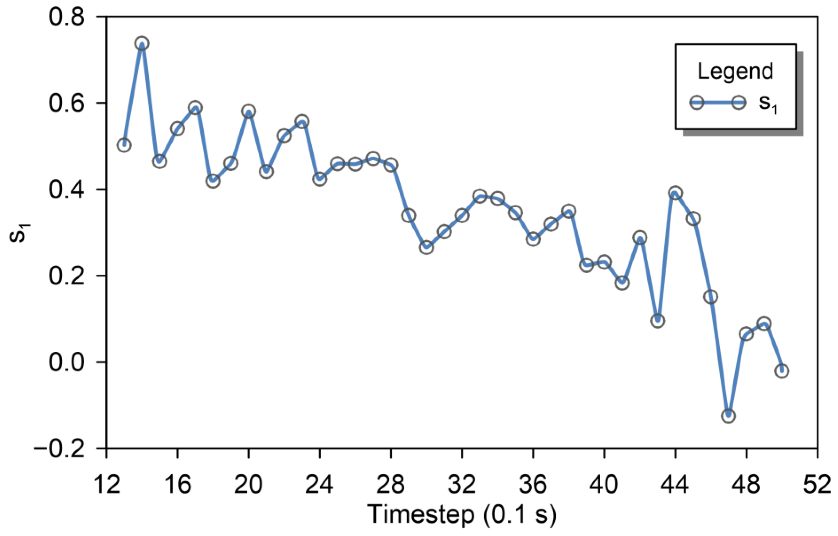
Because the peak flow of debris flow is concentrated within the first 50 timesteps, the subsequent flow through the monitoring point is small fluid. In order to avoid the error effect caused by too few particles, only the velocity profiles of the first 50 timesteps are taken for analysis. Figure 12 shows the time-varying relationship of calculated from the velocity distribution data at the monitoring point x = 6.0 m. It can be seen that the best fit value of changes. When the debris flow flood peak just reaches the monitoring point, it increases to 0.68 rapidly. Then it gradually decreases with time, and finally stabilizes between −0.2 and 0.2. In the first 50 timesteps, varies from −0.2 to 0.7. It can be seen that it is very difficult to find a constant value of to fit the whole flow process in such a large range of changes. Therefore, the linear distribution model has significant limitations in describing the vertical velocity distribution of debris flow. As can be seen from Figure 4, the velocity profile presents a very obvious nonlinear distribution.
However, the proposed velocity nonlinear distribution model still has limitations in reflecting the time-varying relationship of the velocity profile, which can be clearly seen in Figure 12. The evolution of the debris flow velocity profile with time will affect the accuracy of entrainment process estimation. Authors have said that such a limitation will be the next step toward making the presented model perform better for the calculation of basal velocity and estimation of entrainment of debris flow.
6.2. Uniform Particle Simplification
Debris flow shows complex physical characteristics because of its complex particle size composition. Many studies show that the physical characteristics of debris flow are related to its particle size composition [21,22]. Due to the limitations of SPH numerical simulation methods, it is difficult to simulate non-Newtonian fluids with multiple particle sizes. In this paper, in order to reduce computational complexity, a compromise method is adopted. Debris flow is treated as a single uniform particle, and its complex rheological properties are described by an HBP non-Newtonian fluid constitutive model. The strong phase separation in debris flows by uneven particle size in fluid is not thoroughly considered. The effects of this simplification require further study.
7. Conclusions
In this paper, a particle stratified statistical method based on HBP-SPH is proposed to study the vertical distribution of debris flow velocity. In this method, debris flow is simulated by the SPH method integrating the HBP constitutive model. In order to obtain the velocity profile of debris flow, we proposed a particle stratified statistical method. A large number of particle data are analyzed to calculate the average particle velocity within each height layer. A new velocity distribution model based on the logarithm function is presented. The vertical distribution model of velocity is more accurate to describe the nonlinear distribution characteristics of velocity in the depth direction.
In order to verify the proposed method, the large-scale debris flow flume test of USGS was simulated and its 3D dynamic process was inverted. The results show that the proposed method successfully simulates the complex dynamic process of debris flow. By regression analysis of the velocity profile at different times, a nonlinear velocity distribution model based on parameter is proposed. The model is integrated into the existing calculation framework of debris flow erosion depth. A flume dam break test case is used to verify the validity of the framework. The results show that the average erosion depth error of each point in the erosion area is only 15.1%, which proves the validity of the erosion calculation method.
Author Contributions
Z.H. lead the research program, Y.L. designed the simulation. Z.H. and C.Z. wrote the manuscript. Y.L. reviewed and edited the manuscript. All authors have read and agreed to the published version of the manuscript.
Funding
This study was funded by the National Key R&D Program of China (grant number 2018YFD1100401); the National Natural Science Foundation of China (grant number 52078493); the Natural Science Foundation for Outstanding Youth of Hunan Province (grant number 2021JJ20057); the Innovation Provincial Program of Hunan Province (grant number 2020RC3002); the Scientific and Technological Project of Changsha (grant number kq2106018).
Institutional Review Board Statement
Not applicable.
Informed Consent Statement
Not applicable.
Data Availability Statement
The data used in this study are available on request from the corresponding author.
Conflicts of Interest
The authors declare no conflict of interest.
References
- Iverson, R.M.; Reid, M.E.; Logan, M.; LaHusen, R.G.; Godt, J.W.; Griswold, J.P. Positive feedback and momentum growth during debris-flow entrainment of wet bed sediment. Nat. Geosci. 2011, 4, 116–121. [Google Scholar] [CrossRef]
- Johnson, C.G.; Kokelaar, B.P.; Iverson, R.M.; Logan, M.; LaHusen, R.G.; Gray, J.M.N.T. Grain-size segregation and levee formation in geophysical mass flows. J. Geophys. Res.-Earth Surf. 2012, 117. [Google Scholar] [CrossRef]
- Han, Z.; Ma, Y.; Li, Y.; Zhang, H.; Chen, N.; Hu, G.; Chen, G. Hydrodynamic and topography based cellular automaton model for simulating debris flow run-out extent and entrainment behavior. Water Res. 2021, 193, 116872. [Google Scholar] [CrossRef] [PubMed]
- Iverson, R.M. Elementary theory of bed-sediment entrainment by debris flows and avalanches. J. Geophys. Res.-Earth Surf. 2012, 117. [Google Scholar] [CrossRef]
- Han, Z.; Chen, G.; Li, Y.; Tang, C.; Xu, L.; He, Y.; Wang, W. Numerical simulation of debris-flow behavior incorporating a dynamic method for estimating the entrainment. Eng. Geol. 2015, 190, 52–64. [Google Scholar] [CrossRef]
- He, S.; Liu, W.; Li, X. Prediction of impact force of debris flows based on distribution and size of particles. Environ. Earth Sci. 2016, 75, 1–8. [Google Scholar] [CrossRef]
- Ma, Z.; Zhang, J.; Liao, H. Numerical simulation of viscous debris flow block engineering. Rock Soil Mech. 2007, 28, 389–392. (In Chinese) [Google Scholar] [CrossRef]
- Iverson, R.M.; Vallance, J.W. New views of granular mass flows. Geology 2001, 29, 115–118. [Google Scholar] [CrossRef]
- Tecca, P.R.; Deganutti, A.M.; Genevois, R.; Galgaro, A. Velocity distributions in a coarse debris flow. In Debris-Flow Hazards Mitigation: Mechanics, Prediction, and Assessment, Proceedings of the 3rd International Conference; Rickenmann, D., Chen, C.-L., Eds.; Millpress: Rotterdam, The Netherlands, 2003; pp. 905–916. [Google Scholar]
- Ferguson, R. Flow resistance equations for gravel-and boulder-bed streams. Water Resour. Res. 2007, 43. [Google Scholar] [CrossRef] [Green Version]
- Termini, D.; Fichera, A. Experimental Analysis of Velocity Distribution in a Coarse-Grained Debris Flow: A Modified Bagnold’s Equation. Water 2020, 12, 1415. [Google Scholar] [CrossRef]
- Wei, F.; Yang, H.; Hu, K.; Chernomorets, S. Measuring internal velocity of debris flows by temporally correlated shear forces. J. Earth Sci. 2012, 23, 373–380. [Google Scholar] [CrossRef]
- Takahashi, T. Mechanical characteristics of debris flow. J. Hydraul. Eng. 1978, 104, 1153–1169. [Google Scholar] [CrossRef]
- Takahashi, T. Debris flow on prismatic open channel. J. Hydraul. Eng. 1980, 106, 381–396. [Google Scholar] [CrossRef]
- Egashira, S.; Ashida, K.; Yajima, H.; Takahama, J. Constitutive equation of debris flow. Annu. Disaster Prev. Res. Inst. Kyoto Univ. 1989, 32, 487–501. [Google Scholar]
- Hotta, N.; Miyamoto, K.; Suzuki, M.; Ohta, T. Pore-water pressure distribution of solid-water phase flow in a rolling mill. J. Jpn. Soc. Eros. Cont. Eng. 1998, 50, 11–16. [Google Scholar] [CrossRef]
- Drago, M. A coupled debris flow–turbidity current model. Ocean Eng. 2002, 29, 1769–1780. [Google Scholar] [CrossRef]
- Han, Z.; Chen, G.; Li, Y.; Wang, W.; Zhang, H. Exploring the velocity distribution of debris flows: An iteration algorithm based approach for complex cross-sections. Geomorphology 2015, 241, 72–82. [Google Scholar] [CrossRef]
- Han, Z.; Wang, W.; Li, Y.; Huang, J.; Su, B.; Tang, C.; Qu, X. An integrated method for rapid estimation of the valley incision by debris flows. Eng. Geol. 2018, 232, 34–45. [Google Scholar] [CrossRef]
- Han, Z.; Su, B.; Li, Y.; Dou, J.; Wang, W.; Zhao, L. Modeling the progressive entrainment of bed sediment by viscous debris flows using the three-dimensional SC-HBP-SPH method. Water Res. 2020, 182, 116031. [Google Scholar] [CrossRef]
- Domnik, B.; Pudasaini, S.P. Full two-dimensional rapid chute flows of simple viscoplastic granular materials with a pressure-dependent dynamic slip-velocity and their numerical simulations. J. Non-Newton. Fluid Mech. 2012, 173, 72–86. [Google Scholar] [CrossRef]
- Domnik, B.; Pudasaini, S.P.; Katzenbach, R.; Miller, S.A. Coupling of full two-dimensional and depth-averaged models for granular flows. J. Non-Newton. Fluid Mech. 2013, 201, 56–68. [Google Scholar] [CrossRef]
- Calomino, F.; Alfonsi, G.; Gaudio, R.; D’Ippolito, A.; Lauria, A.; Tafarojnoruz, A.; Artese, S.J.W. Experimental and numerical study of free-surface flows in a corrugated pipe. Water 2018, 10, 638. [Google Scholar] [CrossRef] [Green Version]
- Lauria, A.; Alfonsi, G.; Tafarojnoruz, A.J.F. Flow pressure behavior downstream of ski jumps. Water 2020, 5, 168. [Google Scholar] [CrossRef]
- Tafarojnoruz, A.; Lauria, A. Large eddy simulation of the turbulent flow field around a submerged pile within a scour hole under current condition. Coast Eng. J. 2020, 62, 489–503. [Google Scholar] [CrossRef]
- Huang, Y.; Cheng, H.; Dai, Z.; Xu, Q.; Liu, F.; Sawada, K.; Yashima, A. SPH-based numerical simulation of catastrophic debris flows after the 2008 Wenchuan earthquake. Bull. Eng. Geol. Environ. 2015, 74, 1137–1151. [Google Scholar] [CrossRef]
- Dai, Z.; Huang, Y.; Cheng, H.; Xu, Q. SPH model for fluid–structure interaction and its application to debris flow impact estimation. Landslides 2017, 14, 917–928. [Google Scholar] [CrossRef]
- Wang, W.; Chen, G.; Han, Z.; Zhou, S.; Zhang, H.; Jing, P. 3D numerical simulation of debris-flow motion using SPH method incorporating non-Newtonian fluid behavior. Nat. Hazards 2016, 81, 1981–1998. [Google Scholar] [CrossRef]
- Han, Z.; Su, B.; Li, Y.; Wang, W.; Wang, W.; Huang, J.; Chen, G. Numerical simulation of debris-flow behavior based on the SPH method incorporating the Herschel-Bulkley-Papanastasiou rheology model. Eng. Geol. 2019, 255, 26–36. [Google Scholar] [CrossRef]
- Han, Z.; Su, B.; Li, Y.; Wang, W.; Wang, W.; Huang, J.; Chen, G. Smoothed particle hydrodynamic numerical simulation of debris flow process based on Herschel-Bulkley-Papanastasiou constitutive model. Rock Soil Mech. 2019, 40, 477–485. (In Chinese) [Google Scholar] [CrossRef]
- Pudasaini, S.P. A general two-phase debris flow model. J. Geophys. Res.-Earth Surf. 2012, 117. [Google Scholar] [CrossRef]
- Kafle, J.; Pokhrel, P.R.; Khattri, K.B.; Kattel, P.; Tuladhar, B.M.; Pudasaini, S.P. Submarine landslide and particle transport in mountain lakes, reservoirs and hydraulic plants. Ann. Glaciol. 2016, 57, 232–244. [Google Scholar] [CrossRef] [Green Version]
- Mergili, M.; Emmer, A.; Juřicová, A.; Cochachin, A.; Fischer, J.T.; Huggel, C.; Pudasaini, S.P. How well can we simulate complex hydro-geomorphic process chains? The 2012 multi-lake outburst flood in the Santa Cruz Valley (Cordillera Blanca, Perú). Earth Surf. Process. Landf. 2018, 43, 1373–1389. [Google Scholar] [CrossRef] [PubMed]
- Wu, W.; Wang, X.; Zhu, H.; Shou, K.J.; Lin, J.S.; Zhang, H. Improvements in DDA program for rockslides with local in-circle contact method and modified open-close iteration. Eng. Geol. 2020, 265, 105433. [Google Scholar] [CrossRef]
- Zhou, J.; Li, Y.X.; Jia, M.C.; Li, C.N. Numerical simulation of failure behavior of granular debris flows based on flume model tests. Sci. World J. 2013, 2013, 603130. [Google Scholar] [CrossRef] [Green Version]
- Zhang, B.; Huang, Y.; Lu, P.; Li, C. Numerical Investigation of Multiple-Impact Behavior of Granular Flow on a Rigid Barrier. Water 2020, 12, 3228. [Google Scholar] [CrossRef]
- Wang, W.; Yin, K.; Chen, G.; Chai, B.; Han, Z.; Zhou, J. Practical application of the coupled DDA-SPH method in dynamic modeling for the formation of landslide dam. Landslides 2019, 16, 1021–1032. [Google Scholar] [CrossRef]
- Price, D.J. Resolving high Reynolds numbers in smoothed particle hydrodynamics simulations of subsonic turbulence. Mon. Not. Roy. Astron. Soc. 2012, 420, L33–L37. [Google Scholar] [CrossRef] [Green Version]
- Meister, M.; Burger, G.; Rauch, W. On the Reynolds number sensitivity of smoothed particle hydrodynamics. J. Hydraul. Res. 2014, 52, 824–835. [Google Scholar] [CrossRef] [Green Version]
- Sakai, Y.; Hotta, N. Laminar-turbulent transition in debris flow: Measurement of basal pore fluid pressure in an open channel flow experiment. In Proceedings of the EGU General Assembly Conference Abstracts, Online, 4 May 2020; p. 4345. [Google Scholar] [CrossRef]
- Jakob, M.; Hungr, O.; Jakob, D.M. Debris-Flow Hazards and Related Phenomena; Springer: Berlin, Germany, 2005; Volume 739. [Google Scholar]
- Li, S.; Peng, C.; Wu, W.; Wang, S.; Chen, X.; Chen, J.; Chitneedi, B.K. Role of baffle shape on debris flow impact in step-pool channel: An SPH study. Landslides 2020, 17, 2099–2111. [Google Scholar] [CrossRef]
- Huang, Y.; Zhang, W.; Xu, Q.; Xie, P.; Hao, L. Run-out analysis of flow-like landslides triggered by the Ms 8.0 2008 Wenchuan earthquake using smoothed particle hydrodynamics. Landslides 2012, 9, 275–283. [Google Scholar] [CrossRef]
- Naef, D.; Rickenmann, D.; Rutschmann, P.; McArdell, B.W. Comparison of flow resistance relations for debris flows using a one-dimensional finite element simulation model. Nat. Hazards Earth Syst. Sci. 2006, 6, 155–165. [Google Scholar] [CrossRef] [Green Version]
- Chen, H.; Hu, K.; Cui, P.; Chen, X. Investigation of vertical velocity distribution in debris flows by PIV measurement. Geomat. Nat. Hazards Risk 2017, 8, 1631–1642. [Google Scholar] [CrossRef] [Green Version]
- Spinewine, B.; Zech, Y. Small-scale laboratory dam-break waves on movable beds. J. Hydraul. Res. 2007, 45 (Suppl. 1), 73–86. [Google Scholar] [CrossRef]
Figure 1.
Illustration of particle stratification statistics method.
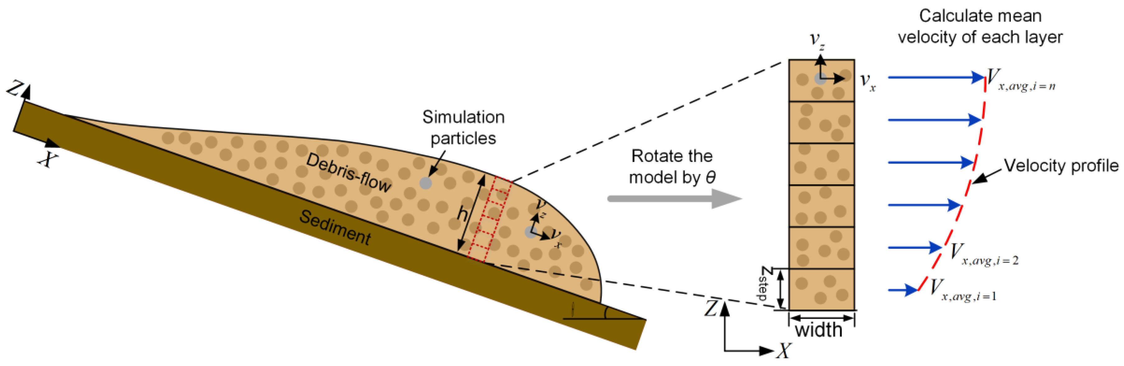
Figure 2.
Numerical model for debris flow flume test.
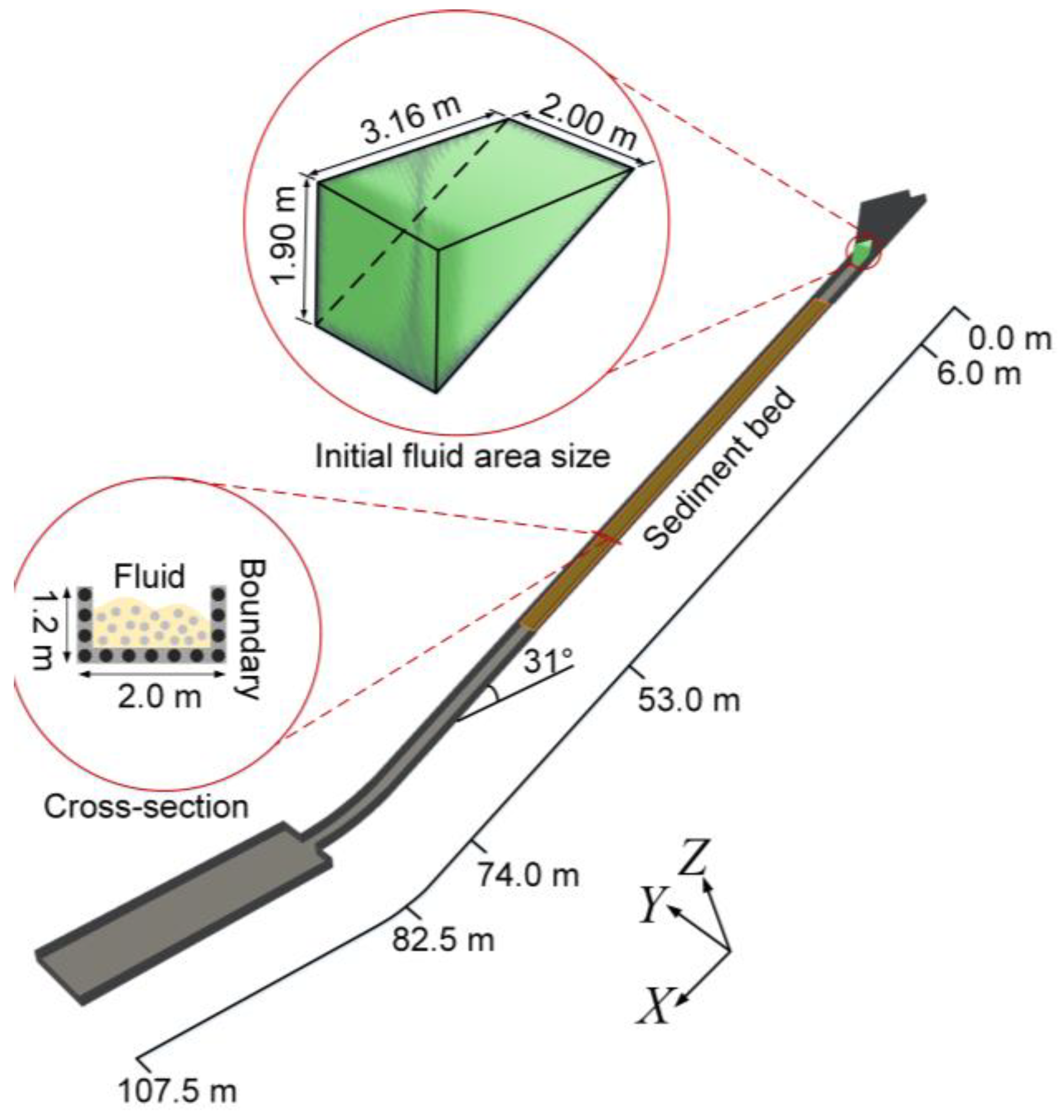
Figure 3.
Flow front position at different times.
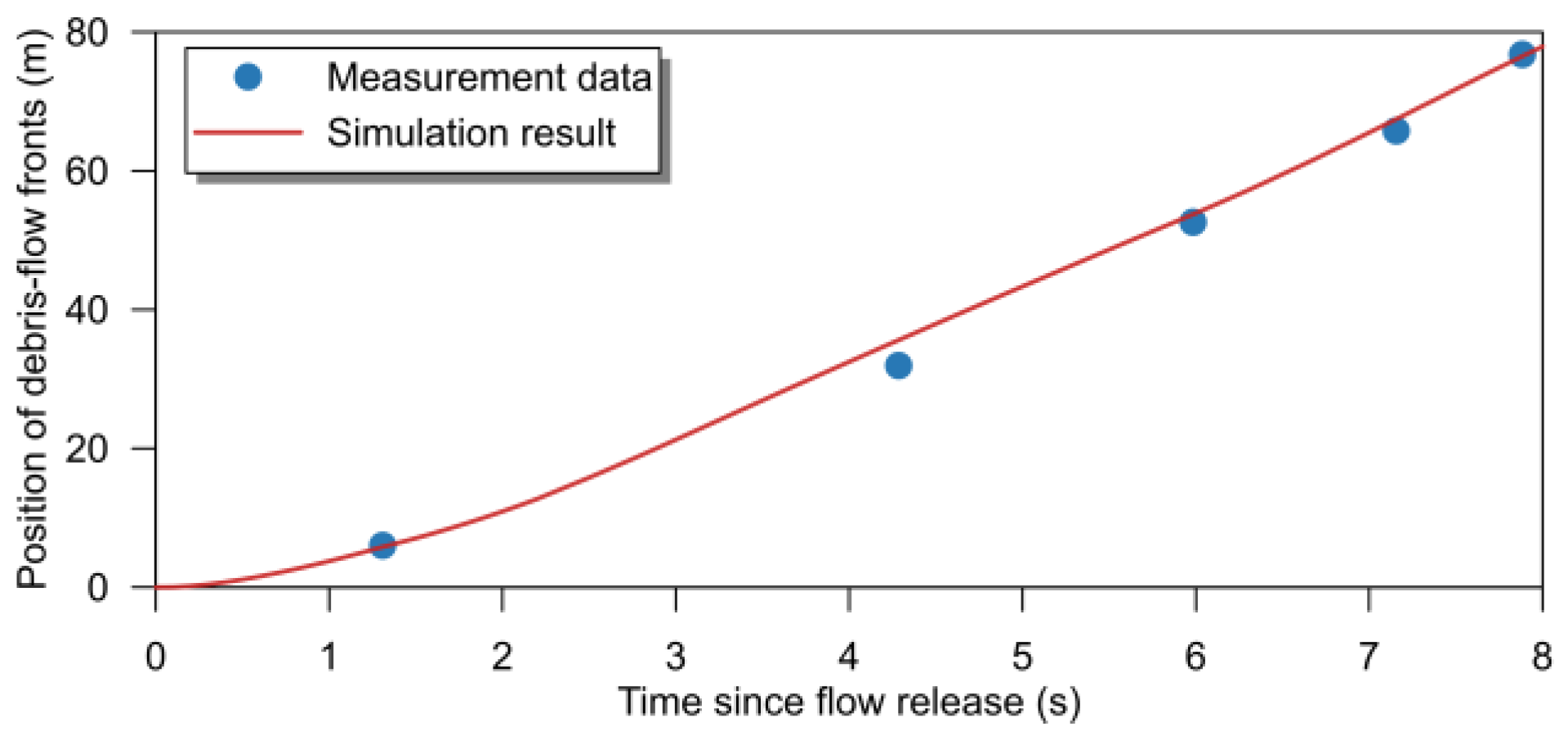
Figure 4.
The result of velocity profile in four timesteps. (a) The number of particles over time. (b) The velocity profile at timestep = 14. (c) The velocity profile at timestep = 16. (d) The velocity profile at timestep = 24. (e) The velocity profile at timestep = 32.
Figure 4.
The result of velocity profile in four timesteps. (a) The number of particles over time. (b) The velocity profile at timestep = 14. (c) The velocity profile at timestep = 16. (d) The velocity profile at timestep = 24. (e) The velocity profile at timestep = 32.

Figure 5.
The boxplot of the single-layer particle velocity profile.

Figure 6.
Velocity profile fitting regression analysis. (a) Regression analysis of velocity profile at timestep = 14. (b) Regression analysis of velocity profile at timestep = 16.
Figure 6.
Velocity profile fitting regression analysis. (a) Regression analysis of velocity profile at timestep = 14. (b) Regression analysis of velocity profile at timestep = 16.

Figure 7.
Analysis of the parameter of the fitting function.
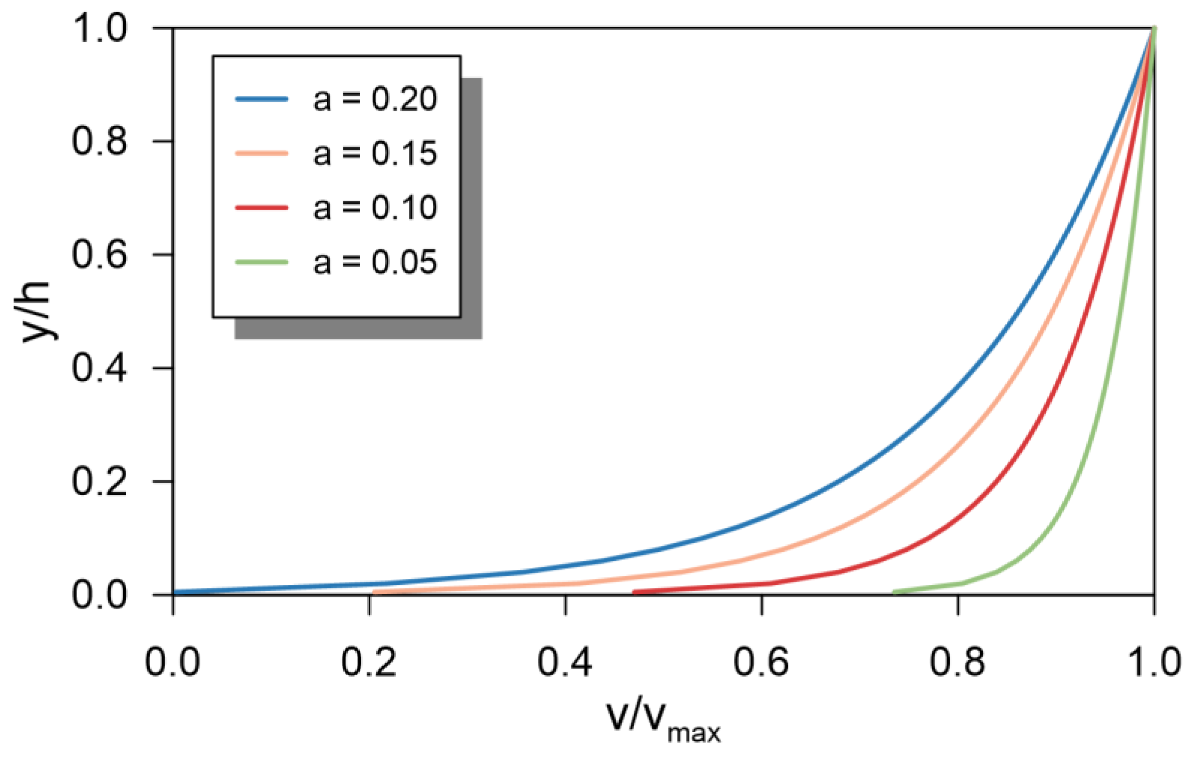
Figure 8.
Diagram of relationship between base velocity and mean velocity.
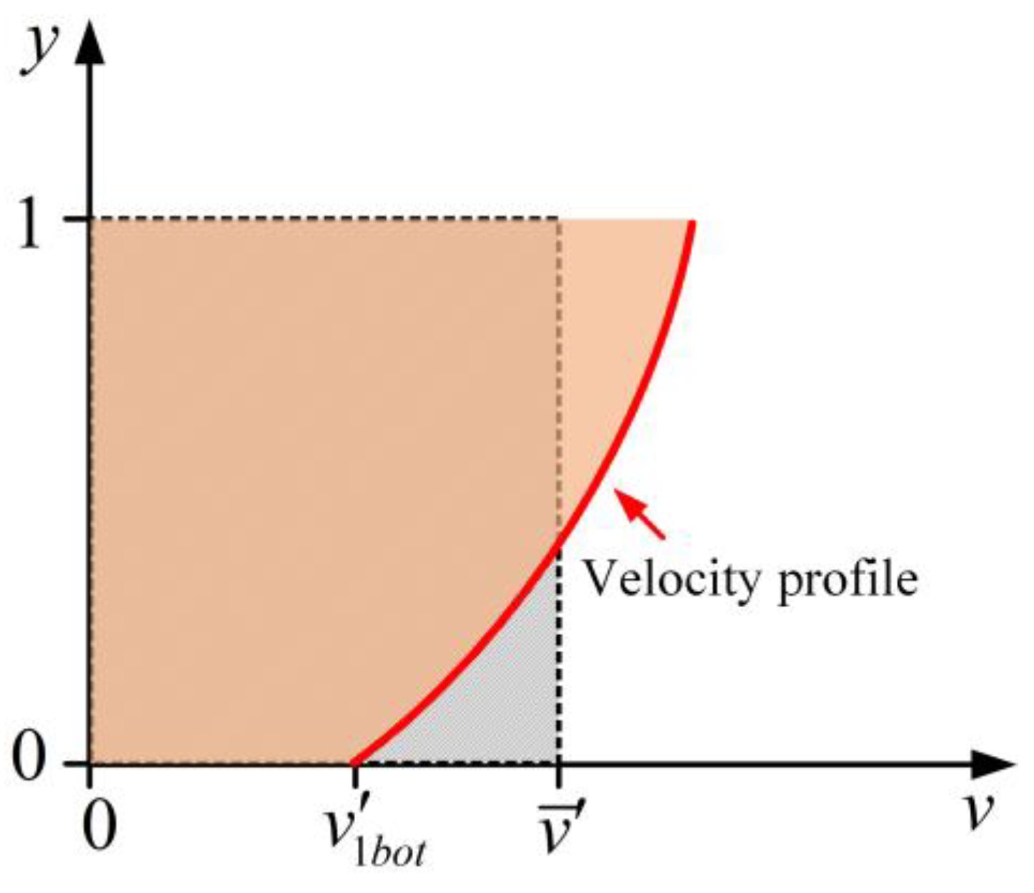
Figure 9.
Schematic diagram of dam break test model size.
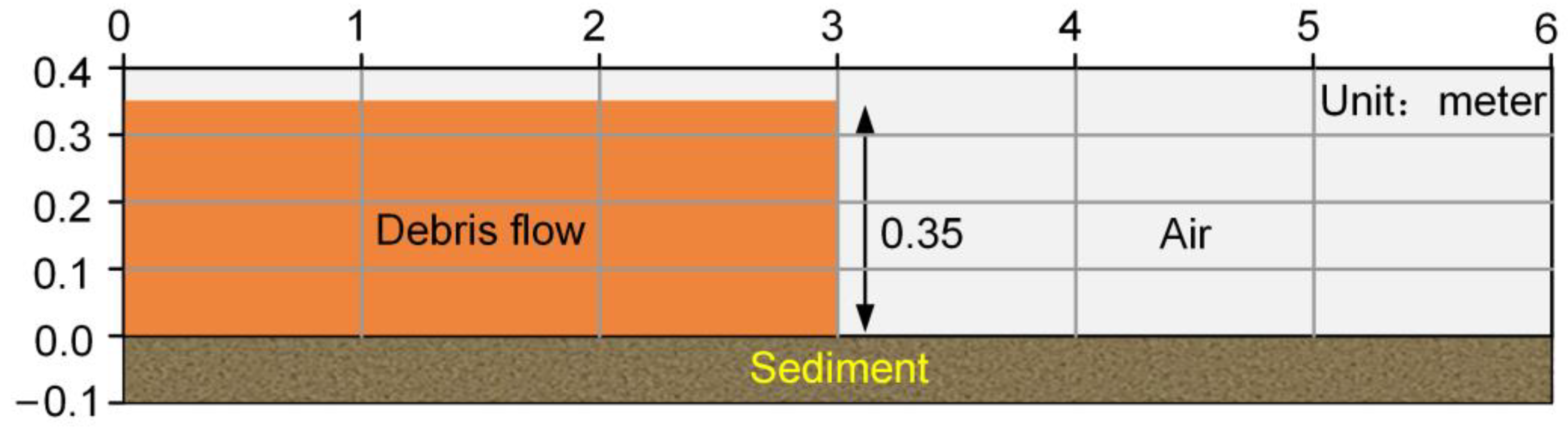
Figure 10.
Erosion depth distribution at different time.
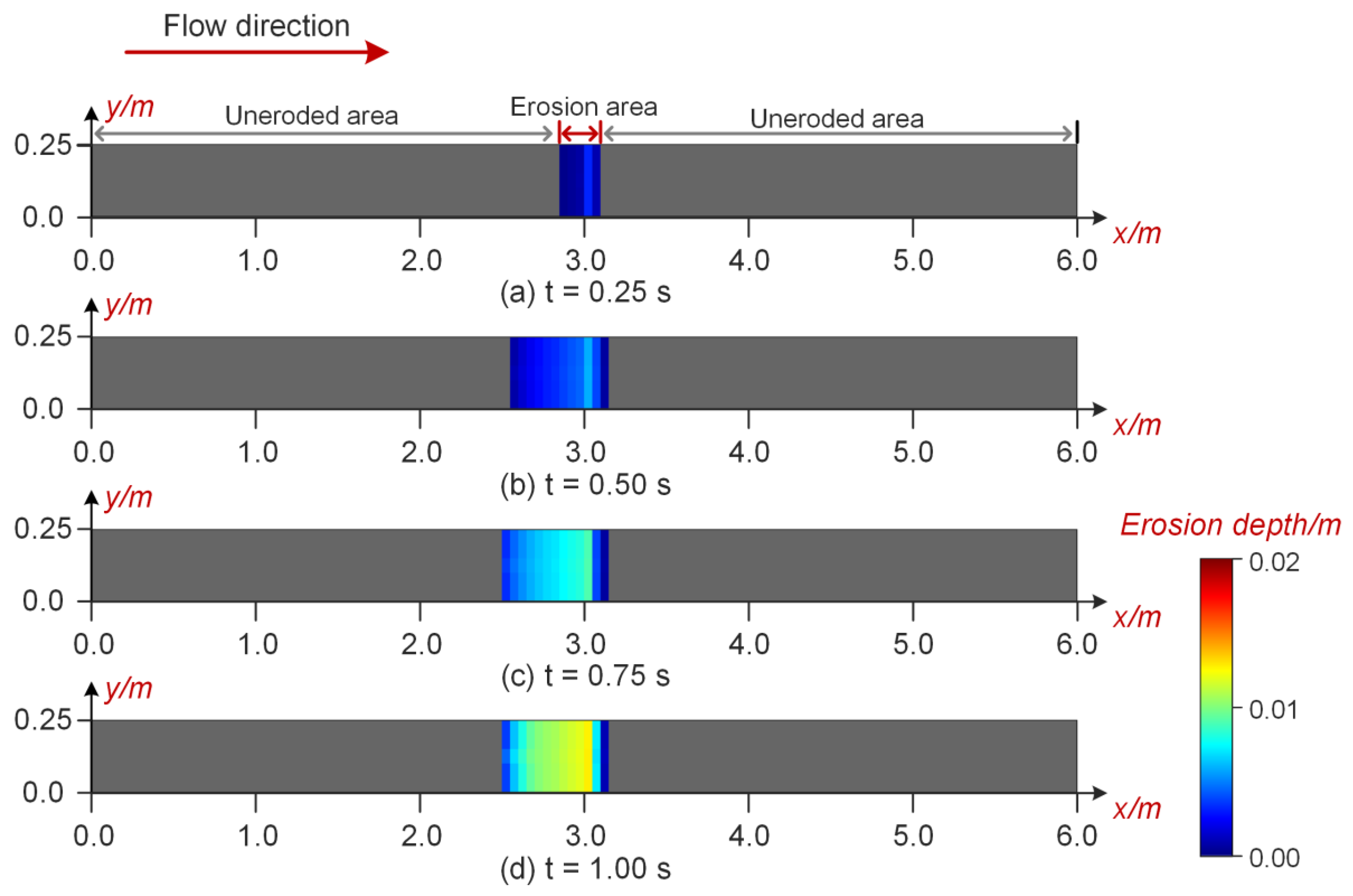
Figure 11.
Erosion depth distribution at different locations at t = 1.5 s. (a) Comparison of experimental data and numerical simulation results. (b) Error percentage of erosion depth numerical simulation results.
Figure 11.
Erosion depth distribution at different locations at t = 1.5 s. (a) Comparison of experimental data and numerical simulation results. (b) Error percentage of erosion depth numerical simulation results.

Figure 12.
The relationship between and time.

Table 1.
Key parameter of numerical simulation.
| Parameter | Notation | Unit | Value |
|---|---|---|---|
| Density of debris flow | kg/m3 | 1650 | |
| Apparent dynamic viscosity | Pa·s | 0.001 | |
| Yield strength | c | Pa | 0 |
| ° | 40 | ||
| Key coefficients of HBP model | / | 100 | |
| / | 1.00 | ||
| Particle distance | m | 0.04 | |
| Smoothing length | m | 0.0866 | |
| Total number of fluid particles | / | 87,591 | |
| Total number of boundary particles | / | 486,694 | |
| Debris flow duration | s | 25 | |
| Initial time interval | s | 0.00001 |
Publisher’s Note: MDPI stays neutral with regard to jurisdictional claims in published maps and institutional affiliations. |
© 2022 by the authors. Licensee MDPI, Basel, Switzerland. This article is an open access article distributed under the terms and conditions of the Creative Commons Attribution (CC BY) license (https://creativecommons.org/licenses/by/4.0/).
Share and Cite
MDPI and ACS Style
Han, Z.; Zeng, C.; Li, Y. Hierarchical Statistics-Based Nonlinear Vertical Velocity Distribution of Debris Flow and Its Application in Entrainment Estimation. Water 2022, 14, 1352. https://doi.org/10.3390/w14091352
AMA Style
Han Z, Zeng C, Li Y. Hierarchical Statistics-Based Nonlinear Vertical Velocity Distribution of Debris Flow and Its Application in Entrainment Estimation. Water. 2022; 14(9):1352. https://doi.org/10.3390/w14091352
Chicago/Turabian StyleHan, Zheng, Chuicheng Zeng, and Yange Li. 2022. "Hierarchical Statistics-Based Nonlinear Vertical Velocity Distribution of Debris Flow and Its Application in Entrainment Estimation" Water 14, no. 9: 1352. https://doi.org/10.3390/w14091352
Note that from the first issue of 2016, this journal uses article numbers instead of page numbers. See further details here.