
Agricultural Total Water Consumption Coefficient and Its Spatial Correlation Network in Yangtze River Economic Belt

1
College of Sciences, North China University of Science and Technology, Tangshan 063210, China
2
College of Water Sciences, Beijing Normal University, Beijing 100875, China
3
South to North Water Transfer Planning and Design Administration, Ministry of Water Resources, Beijing 100038, China
4
Changjiang River Scientific Research Institute, Changjiang Water Resources Commission, Wuhan 430010, China
5
Hubei Provincial Key Laboratory of Basin Water Resources and Ecological Environment, Changjiang River Scientific Research Institute, Wuhan 430010, China
*
Author to whom correspondence should be addressed.
Water 2023, 15(11), 2055; https://doi.org/10.3390/w15112055
Submission received: 24 March 2023
/
Revised: 18 May 2023
/
Accepted: 26 May 2023
/
Published: 29 May 2023
(This article belongs to the Special Issue Sustainable Management of Agricultural Water)
Abstract
:Agriculture contributes extensively to the economic development of countries; however, it is one of the main water-consuming industries. Revealing the characteristics and network structure of agricultural water use efficiency (AWUE) is conducive to green and coordinated development of agriculture. Considering that analyzing the variation of AWUE is helpful to calculating the AWUE, this study aims to calculate the total water consumption coefficient of the agricultural sector in the Yangtze River Economic Belt (YEB) by using the China interregional input-output tables in 2012 and 2017. The gravity model was modified to deduce the spatial correlation network of agricultural total water consumption coefficient (ATWCC), and the social network analysis method was used to analyze the network structural characteristics. The results show that: (1) compared to 2012, the AWUE of YEB in 2017 improved, with a decrease of ATWCC from 532.5 to 387.5 m3/10,000-yuan, account for 27.2%; (2) The network relevance of ATWCC of YEB’s 11 provinces (cities) enhanced, the rank relationship within the network and the network structure was relatively stable; (3) The spatial correlation network formed several network centers, Zhejiang and Jiangsu in the eastern coastal area were the main destinations of the spatial spillover of the spatial correlation network.
1. Introduction
Agriculture is an irreplaceable important sector that highly relies on water resources [1]. However, the global risk of water shortages poses a severe challenge to the sustainable development of agriculture [2]. Thus, it is of great significance to analyze the agricultural water use efficiency (AWUE) and put forward the countermeasures.
At present, the research on AWUE mainly focuses on two aspects: the technical research on improving AWUE [3,4,5,6,7], and the measurement and analysis of AWUE [8,9,10,11]. While the latter reveals existing problems and identifies directions for improvement, the former is aimed at specific implementation.
Measurement and analysis of AWUE have frequently used the data envelopment analysis (DEA) method based on input-output tables [7,9,12]. Recently, combining DEA with other analysis methods has become an important research direction. Shi et al. coupled the DEA model and Social Network Analysis (SNA) to evaluate the AWUE of YEB from 2010 to 2019 [11]. Zhang et al. adopted a slacked-based model to measure China’s AWUE [13], etc. As the economy and society developed, the relationship among regions or sectors becomes increasingly interconnected, and water flow becomes more frequent. However, current AWUE research primarily focuses on direct water use in the agricultural sector, neglecting the virtual water consumption of other sector products used by the agricultural sector. Xu et al. put forward the calculation method of direct water consumption coefficient (DWCC) and total water consumption coefficient (TWCC) [14], which provides a solution to deal with this issue.
According to Xu et al. [14], the water resources calculated in DWCC are mainly natural forms, but water resources involved both the virtual form and the real form. In actual production, not only are a large number of natural form water resources consumed by the different sectors, but tons of virtual water are also consumed through the exchange of products and services. The two parts of water resource constitute TWCC, which refers to the total water resource consumed by the whole economic system to increase one unit of products in a sector. TWCC has become an important tool to account for the virtual water and optimize the industrial structure [15,16,17,18]. It is worth emphasizing that the characteristics of TWCC mentioned above make it a more objective indicator for measuring AWUE. Specifically, the larger the TWCC value, the lower the AWUE of the agricultural sector. Therefore, the agricultural total water consumption coefficient (ATWCC) is a crucial tool for objectively and comprehensively assessing AWUE, which has received limited attention in current research. Furthermore, with the advancement of regional coordinated development strategies, the flow of labor, capital, technology, products, and virtual resources among regions has accelerated [19]. The spatial correlation between regional industries and consumption has surpassed geographical proximity limitations, forming a spatial correlation network. At present, spatial association network analysis has become one of the important research contents for regional coordination and sustainable development [20,21,22]. Therefore, revealing the spatial correlation network of AWUE is helpful for the formulation and implementation of relevant policies and measures.
As an important component of social and economic activities, the spatial effects of agricultural water use may also exceed geographical proximity and create a spatial correlation network. However, few studies have been conducted within this field. As one of China’s important strategic development areas, the Yangtze River Economic Belt (YEB), which spans the East, middle, and west of China, covers six of 13 major grain-producing areas. YEB plays a crucial role in China’s agricultural production and coordinated development. Therefore, based on the above analysis, considering YEB as the research area, this study aims to explore ATWCC and its spatial correlation network, and provide support for YEB’s agricultural sector water resources utilization and management.
2. Materials and Methods
2.1. Study Area
YEB is a major strategic development area in China, including 11 provinces (cities) (Figure 1) (Sichuan, Guizhou, Yunnan and Chongqing; Hubei, Hunan and Jiangxi; Shanghai, Jiangsu, Zhejiang and Anhui). The total area of YEB is about 2.05 × 10⁶ km2, accounting for 21.4% of China [23]. YEB has abundant water resources, which account for more than 40% of China’s total. YEB is the largest food production and processing base in China, which has six provinces (cities) in China, namely Jiangsu and Anhui in the upper reaches, three provincial administrative regions in the middle reaches, and Sichuan in the lower reaches [24]. YEB plays an important role in ensuring China’s food security. However, agricultural water use efficiency in YEB is low. In 2017, the food-sowing area of YEB accounted for 36.5% of China, while the water-saving irrigation area accounted for only 27.3%. The water-saving irrigation area was 9.38 × 10⁶ hm2, accounting for only 21.75% of the food sowing area. Therefore, studying AWUE and its network structure in YEB is of great practical significance.
2.2. Data Preparation
To account for water consumption in the agricultural sector (Agriculture, forestry, animal husbandry, and fishery), the interregional input-output table of 31 provinces (cities, autonomous regions) in China was utilized.
The areas outside YEB were aggregated as “China outside YEB”. The balance rule was applied to verify the Input-Output table, ensuring that the total input equals the total output [25], as shown in Table 1.
All the data involved in this study are from the water resources bulletin and statistical yearbook of China and each province (city) in YEB (2012 and 2017); Economic census yearbook, energy statistical yearbook, wine sector yearbook, agricultural products processing sector yearbook of China (2013 and 2018) and EPS data platform.
2.3. Agricultural Total Water Consumption Coefficient (ATWCC)
The input–output analysis is a common analysis method in Econometrics [26], since 1960, it has been widely used in the research of leading sectors and industrial linkages [14,25], resource circulation and environmental impact [27]. To quantify the agricultural water consumption in the 11 provinces (cities) of YEB, the inter provincial circulation relations must be considered. Therefore, it is necessary to use the Multi-Regional Input–Output (MRIO) model for accounting.
The MRIO table of water consumption for YEB was constructed (Table 1). The monetary unit is 10,000-RMB yuan. There are 12 regions, , representing Shanghai, Jiangsu, Zhejiang, Anhui, Jiangxi, Hubei, Hunan, Chongqing, Sichuan, Guizhou, Yunnan and the areas outside YEB in China. Each region has n sectors, . The row balance relationship is as follows [26].
where, and are any two regions. is the total output of sector in the region . is the intermediate input provided by sector of region to sector of region ; is the input of sector in region to the final demand of region . is the output of sector in region .
The direct water consumption coefficient (DWCC) is as follows:
Bring Formula (2) into Formula (1):
Expressed as the matrix form:
Further,
where, is Leontief inverse matrix. is the input of sector to meet the production needs of a unit product of sector in region .
To establish the connection between economic and water resources data, water resource consumption was introduced into the MRIO table. The DWCC represents the total amount of water resources invested by each sector in the process of producing a unit of product [14], and the formula is:
where, refers to the total amount of the water resource to be consumed in unit products or services of sector in region . refers to the amount of water resources consumed by sector in region ; is the total output of sector in region .
According to DWCC, the TWCC can be calculated as follows:
2.4. Modified Gravity Model
To identify whether the ATWCC of 11 provinces (cities) in YEB has spatial correlation network characteristics, it is necessary to construct the gravity matrix in the first place. According to the relative research works [20,28], a modified gravity model to measure the spatial correlation gravity intensity of ATWCC was constructed as follow:
where, refers to the gravity of ATWCC between the and provinces (cities) of YEB. , , , , and respectively refers to the ATWCC, agricultural GDP and agricultural GDP per agricultural worker in the and provinces (cities). refers to the geographical distance obtained by the ArcGIS distance tool between the and provinces (cities).
After calculating gravity, the spatial correlation network matrix can be constructed. Here, taking the mean value of gravitation in each row as the comparison value, those greater than the average level are recorded as 1, otherwise as 0.
2.5. Social Network Analysis (SNA)
SNA is a scientific method to analyze the correlation networks based on “relationship data”, which has been widely used in many fields [29,30,31,32,33]. This study uses SNA to analyze the structural characteristics of the ATWCC spatial correlation network in YEB. This characteristic is mainly analyzed by five indicators: network relationships number, density, correlation, rank and efficiency. The network relationships number refers to the actual relationships number between different provinces (cities). When the network relationships number is greater, the network density is greater, indicating that the ATWCC of 11 provinces (cities) is more closely related, and the impact of ATWCC among provinces (cities) is also stronger. The network density can be calculated as follows:
where, and represent the number of provinces (cities) and the network relationships respectively.
The network correlation reflects the robustness of the network. When it is 1, it indicates that the ATWCC of 11 provinces (cities) has a spatial network effect, and the network is robust. The calculation formula is:
where, refers to the number of unreachable point pairs.
The network rank reflects the status difference of ATWCC in 11 provinces (cities). The higher the rank, the greater the rank difference formed in the spatial correlation network. The calculation formula of network rank is:
where, and denote the number of symmetric reachable point pairs and the number of maximum symmetric reachable point pairs respectively.
The network efficiency reflects the stability of the network. A lower network efficiency indicates a more stable spatial correlation network. The calculation formula for network efficiency is:
where, and represent the number of redundant links between provinces(cities) and the number of maximum possible redundant links, respectively.
The individual characteristic of spatial correlation networks is mainly analyzed by three indicators: point center degree (PCD), closeness center degree (CCD) and intermediation center degree (ICD). PCD is used to measure the number of other provinces connected to a province in the network, which can be divided into point-out degrees and point-in degrees. In this study, the higher the PCD, the closer the province (city) is to the network center, and the stronger its effect on other network nodes. There are two measurement methods: absolute and relative.
Relative PCD is the most commonly used, which can be expressed as:
CCD is used to describe the degree to which a province(city) is not controlled by others. If the distance between a province(city) and others is short, it has more obvious advantages in transmitting information, and its closeness to the center will be higher. When a province (city) is closer to the center, it indicates that it is closer to others in the network. The CCD can be expressed as:
where, refers to the shortcut distance between the and province (city).
ICD is used to measure the intermediary role of a province (city) in other point pairs. If a province (city) is on many other points to point shortcuts, it has a high ICD. When a province (city)’s ICD is higher, it plays a stronger role in controlling and regulating the ATWCC of others in the network. ICD can be expressed as:
where, , and ; indicates the ratio of the number of shortcuts () passing through the province (city) and connecting the and the to the total number of shortcuts between the and ().
Using the plate model analysis method, this paper discusses the role of each plate in the ATWCC spatial correlation network in 11 provinces (cities) of YEB. Referring to the research of WASSERMAN and FAUST [34], the spatial association network is divided into four attributes. The attributes of the plate are judged according to the number of received and issued relationships inside and outside the plate, and the number of members inside the plate (Table 2), revealing the position and role of each plate in the spatial network, as well as the connection and interaction between the internal and external of the plate, in which and represent the number of members in the plate and in the whole network relationship.
Here, the CONCOR algorithm of UCINET 6.0 was used to cluster the ATWCC spatial association network.
3. Results
3.1. ATWCC in YEB in 2012 and 2017
Based on the MRIO model and Equations (2), (6), and (7), the ADWCC and ATWCC of YEB in 2012 and 2017 were calculated, as shown in Figure 2.
Figure 2a,b indicates that the proportion of ADWCC in ATWCC in YEB was relatively high, 80.29% (2012) and 81.30% (2017), which remained basically unchanged. Among them, the proportion in Shanghai in 2017 was as high as 92.51%, which may indicate that the agricultural modernization level in this region is relatively high and it is less dependent on other sectors. Figure 2c,d shows that from 2012 to 2017, both ADWCC and ATWCC in YEB have decreased to a certain extent. Among them, the average value of ADWCC decreased from 427.4 to 315.1 kg/10,000 yuan, with a decrease rate is 26.27%, while the average value of ATWCC decreased from 532.5 to 387.5 kg/10,000-yuan, with a decrease rate is 27.2%.
Regarding sector-wide consumption, Figure 2d shows that the AWUE of YEB has improved in the past five years, and the same agricultural input has obtained more economic output. On the one hand, agricultural production efficiency has been improved under the development of agricultural science and technology. The application of agricultural information technology and new irrigation equipment has improved the AWUE. On the other hand, the awareness of water conservation among agricultural employees has increased with the in-depth promotion of high-quality development and green development strategy, leading to a transformation from extensive water use to intensive water conservation, which has achieved remarkable results.
Based on the data from different provinces and cities in YEB, it was found that ATWCC decreased to varying degrees over the past five years. Guizhou showed the largest decrease, with a downtrend of 48.4%, followed by Chongqing and Hubei with 37.9% and 37.7%, respectively. In 2017, Chongqing had the lowest ATWCC, only 166 kg/10,000-yuan, while Shanghai had the highest, reaching 614.1 kg/10,000 yuan. The main reason for this difference is that Shanghai has a highly developed economy with a low proportion of primary industry, whereas Chongqing has a reasonable industrial structure and relatively high agricultural water technology, being an economically developed municipality directly under the central government and adjacent to three of China’s major grain-producing areas. On the other hand, Jiangxi’s agricultural production is relatively backward compared to Hunan and Hubei and the developed coastal areas in the East, resulting in the largest ATWCC of 619.4 kg/10,000 yuan. Overall, the ATWCC in YEB has been effectively controlled, and the AWUE has been greatly improved. However, there is still room for improvement in the region.
3.2. ATWCC’s Spatial Correlation Network
3.2.1. Overall Characteristics
By taking the ATWCC of 11 provinces (cities) in YEB in 2012 and 2017 as the basic data, a spatial correlation binary matrix of ATWCC for the 11 provinces (cities) in YEB was constructed using a combination of gravity calculations with Equation (8). The UCINET software was then used to create a spatial network topology map of the ATWCC for the 11 provinces (cities) in YEB (Figure 3), and the spatial network structure was analyzed. The results show that the ATWCC in the 11 provinces (cities) of YEB has transcended the traditional spatial geographical proximity overflow attribute. There are no isolated points in the network, and the overall network exhibits the characteristics of a complex spatial correlation network.
Using UCINET 6.0, the overall characteristic indexes of the ATWCC spatial correlation network of 11 provinces (cities) in YEB in 2012 and 2017 are calculated (Table 3).
Table 3 shows a slight upward trend in the number of network relationships in the ATWCC spatial correlation networks of 11 provinces (cities) in YEB, from 28 in 2012 to 32 in 2017, an increase of 14.29%. The network density also increased from 0.255 to 0.291, an increase of 25.88%. These changes indicate that the association intensity between provinces (cities) in terms of ATWCC has increased from 2012 to 2017, and the interaction between them has been strengthened. This can be attributed to the gradual improvement of the market economic system, which has facilitated the circulation of agricultural production and management factors. Additionally, the rapid development of transportation and information networks in YEB has supported agricultural water agglomeration, technology diffusion, and labor transfer, which have strengthened the correlation between agricultural production and operation among provinces (cities) and facilitated the formation of the spatial correlation of ATWCC.
In addition, during these five years, the implementation of the regional development strategy of YEB has accelerated the coordinated development within the region, and also provided impetus and support for the flow of various agricultural factors across the country. From 2012 to 2017, the number of network relationships has improved to a certain extent, but there is still a very large gap compared with the maximum possible total of 110 relationships. Therefore, there is still a lot of room for improvement.
From 2012 to 2017, the network correlation degrees were all 1, showing that all 11 provinces (cities) were included in the network, and the network structure of this spatial correlation network is stable, the ATWCCs of all provinces (cities) are interconnected, and the spatial spillover effect of ATWCC is wide, not limited to the adjacent areas. The network rank is relatively stable, falling from 0.773 in 2012 to 0.746 in 2017, reflecting that the internal rank is obvious and relatively stable. YEB spans the eastern, central, and western regions of China and there are significant regional differences in the level of agricultural development and water resources endowment in the upper, middle, and lower reaches.
Therefore, to achieve coordinated development within the YEB region, it is essential to uphold the fundamental principles of upper and lower reaches, left and right banks co-management, and systematic governance. The overall network efficiency experienced a slight decline from 0.711 in 2012 to 0.689 in 2017, representing a 3.1% decrease and indicating a strengthened network stability. This trend may be attributed to the continued implementation of the national key development strategy of YEB, which has facilitated the coordination of regional economic and social development, resulting in an increased correlation relationship among ATWCC in each province (city). The heightened spatial correlation lines between nodes have brought the network closer together, leading to stable improvement.
3.2.2. Individual Structure Characteristics
Using UCINET 6.0, the individual structure indicators of the ATWCC spatial correlation network in 11 provinces (cities) of YEB in 2017 are calculated (Table 4).
Table 4 shows that the average PCD of the ATWCC spatial correlation network of 11 provinces (cities) in YEB in 2017 was 39.669. Among them, the PCD of Jiangsu, Zhejiang and Chongqing is higher than the average, indicating that these provinces (cities) are closer to the center of the network than other provinces (cities) in the network, and have more connections with other provinces (cities). These provinces (cities) play a key role in the formation and stable development of the overall network. Among them, Jiangsu and Zhejiang are located in developed coastal areas. These areas have advanced agricultural technology, rapid economic development, and convenient transportation network, which enable them to have an important impact on the agricultural economic output of other provinces (cities) through agricultural technology transfer, agricultural investment, absorption of agricultural labor, etc.; Chongqing, the only municipality directly under the central government in Southwest China, is the economic development area in the upper reaches of YEB, and is at the key node connecting the upper and middle reaches. The low PCD of Jiangxi and Shanghai may be mainly due to the geographical location and ultra-high ATWCC. Shanghai’s economy is highly developed, however, in 2017, the proportion of the primary industry was only 0.3%. The higher ATWCC, as high as 614.1 m3/10,000 yuan, was less than that of Jiangxi, which was 619.4 m3/10,000-yuan. From the perspective of network structure, Shanghai has a network relationship with neighbor provinces Jiangsu and Zhejiang, and the situation of Jiangxi and Shanghai remains the same.
4. Discussion
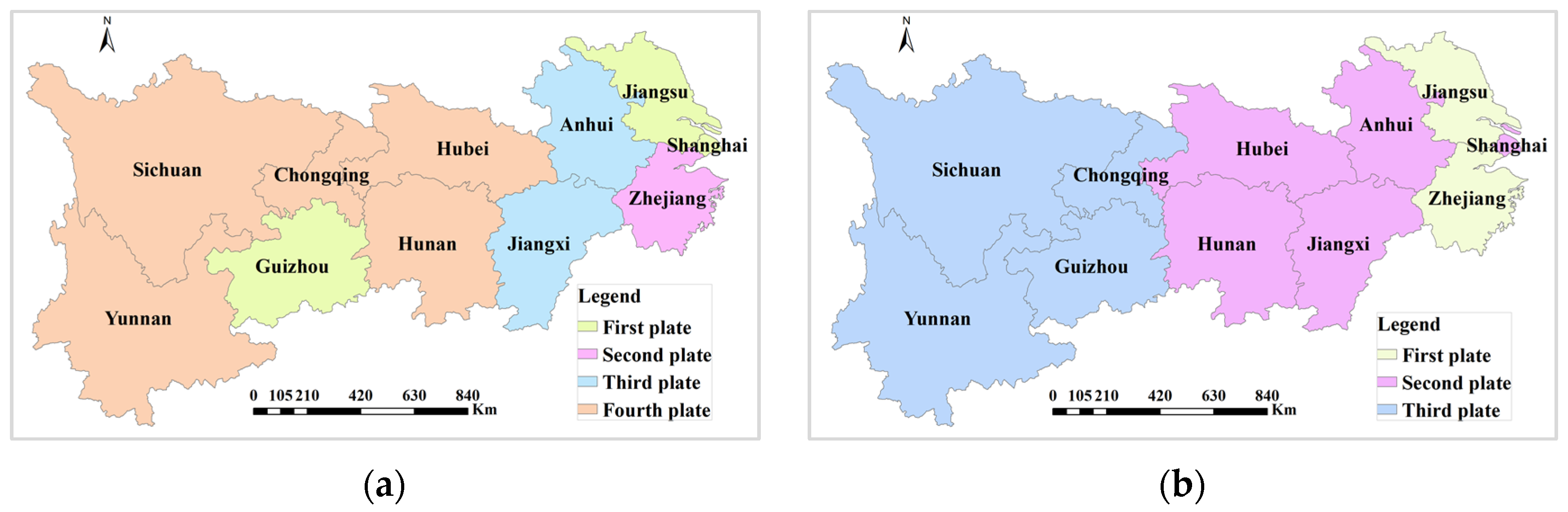
The study uses the CONCOR algorithm to analyze the ATWCC spatial association network of 11 provinces (cities) in YEB. Here, the maximum segmentation density was set to 2 and the convergence standard was set to 0.2. Then, the overall network was respectively divided into four plates (2012) and three plates (2017), as shown in Figure 4.
Figure 4 shows that the ATWCC network structure of YEB has obvious regional characteristics, and this trend is becoming more and more obvious.
In 2017, the division of plates was almost the same as that of upper, middle, and lower reaches., as shown in Table 5.
It can be seen from Table 5 that there are 8 inside plate correlations and 24 outside plate correlations, accounting for 25% and 75% of the total network correlation number in 2017, showing that there are spatial agglomeration effects and spatial spillovers among the provinces (cities) in the ATWCC. Among them, the first plate includes Zhejiang and Jiangsu, with 0 internal relations, 18 received relationships outside the plate, and 5 issued relationships outside the plate. The expected internal relationship ratio is more than the actual internal relationship ratio, making it a net beneficiary region that mainly benefits from the input of factors from other regions. The second plate includes Shanghai, Hunan, Jiangxi, Anhui, and Hubei. It has 3 inside plate relations, 6 received relations outside the plate and 10 issued relationships outside the plate. The expected internal relationship ratio is more than the actual internal relationship ratio. It belongs to the broker plate. It has close spatial relations with both inside and outside plate members and acts as a link for element communication in the spatial correlation network. As an important port and trading venue, Shanghai has close connections with other cities, accompanied by the circulation of virtual water resources for agricultural products. Hunan, Hubei, Jiangxi, and Anhui are located in the central part of YEB, occupying an important geographical connection position, providing convenience for the circulation of products from the east to the west, which to some extent reflects the good regional coordination relationship of YEB as an economic demonstration belt.
The third plate includes 4 provinces (cities), that is, Chongqing, Sichuan, Guizhou and Yunnan, with 9 inside plate relationships, 0 off plate received relationships, and 9 outside plate issued relationships. The expected internal relationship ratio is less than the actual internal relationship ratio, belonging to the net overflow plate. Most of these regions are important provinces (cities) rich in water resources in China. The upper reaches of YEB are rich in natural resources, abundant in water resources, and have good agricultural production conditions. It has taken on important basic support in YEB’s national strategy and coordinated development, delivering a large amount of virtual water resources to the middle and lower reaches.
On this basis, the density matrix of the ATWCC spatial correlation network was calculated by using the condensed subgroup analysis path, and the R-squared is equal to 0.607. Then, the elements in the density matrix that are greater than the density of the ATWCC spatial correlation network of 11 provinces (cities) in YEB in 2017 (0.291 measured above) were recorded as 1, and vice versa, they are 0 to obtain the image matrix (Table 6).
It can be seen that the ATWCC of the second and third plates overflows into the first plate; The ATWCC of the first plate has a certain space overflow to the second plate; The first and the second plate show asymmetric two-way spillover effect; On the whole, Zhejiang and Jiangsu are the main destinations of ATWCC spatial spillovers.
5. Conclusions
In this study, after the interregional input–output tables of 31 provinces (cities, autonomous regions) in China in 2012 and 2017, the water resource consumption row was added, and the input–output table of water resource use in YEB was constructed. Then the ATWCC of YEB was calculated. On this basis, the spatial correlation network structure of ATWCC in 11 provinces (cities) of YEB is analyzed by using a modified gravity model and social network analysis method. The main conclusions are as follows:
- (1)
- from 2012 to 2017, the AWUE in all 11 provinces (cities) of YEB have improved to some extent, especially Guizhou (increase of 48.4%). Zhejiang, Hubei, Chongqing and Yunnan are all more than 30%. For YEB, the ATWCC decreased from 532.5 to 387.5 m3/10,000 yuan, correspondingly, AWUE increased by 27.2%.
- (2)
- ATWCC’s spatial effect presents the characteristics of spatial correlation; the network density shows an upward trend, rising to 0.291 from 0.255, indicating that the ATWCC interaction between provinces (cities) was strengthened. The network structure of this spatial correlation network is stable, the ATWCCs of all provinces (cities) are interconnected, and the spatial spillover effect of ATWCC is wide, not limited to the adjacent areas. The network rank is relatively stable with a little fall of 3.49%, reflecting that the internal rank is obvious and relatively stable. The overall network efficiency showed a slight downward trend, indicating that network stability has been enhanced.
- (3)
- The spatial correlation network has formed several network centers, such as Zhejiang, Chongqing and Jiangsu, which has played an important role in the formation of the spatial correlation network and has an impact and control on ATWCC in the 11 provinces (cities); In terms of cluster structure characteristics, YEB has obvious regional characteristics. Especially in 2017, the division between the upper, middle and lower reaches and the three plates has been basically continuous. Zhejiang and Jiangsu in the eastern coastal area are the main destinations of the spatial spillover of the spatial correlation network.
ATWCC accounting and its network correlation analysis are helpful to reveal the water use situation and complex status of regional agricultural sectors and can provide some decision support for the improvement of AWUE and regional coordinated development. Accurate and timely data acquisition is the premise of ATWCC accounting and the key approach to improving the reliability of results. However, China’s latest interregional input-output table is the 2017 version, which inevitably leads to insufficient timeliness. In any case, this meaningful work will continue after the next version is available.
Author Contributions
Conceptualization, Y.Y. and H.W.; methodology, Y.Y. and Y.G.; software, R.Z. and H.Y.; validation, Y.Y., Y.G. and R.Z.; formal analysis, R.Z.; investigation, J.X.; resources, H.W. and J.X.; data curation, R.Z.; writing—original draft preparation, Y.Y.; writing—review and editing, Y.Y., R.Z. and Y.G.; supervision, J.X. and H.W.; funding acquisition, H.W. and Y.Y. All authors have read and agreed to the published version of the manuscript.
Funding
This research was funded by the CRSRI Open Research Program (Program SN: CKWV20221035/KY), Beijing Natural Science Foundation (8222057), the National Natural Science Foundation of China (52279005), and the 111 Project (Grant No. B18006).
Data Availability Statement
The data that support the findings of this study are available from the corresponding author upon reasonable request.
Conflicts of Interest
The authors declare no conflict of interest.
Abbreviations
| Abbreviation | Meaning |
| AWUE | Agricultural water use efficiency |
| TWCC | Total water consumption coefficient |
| DWCC | Direct water consumption coefficient |
| YEB | Yangtze River Economic Belt |
| ADWCC | Agricultural direct water consumption coefficient |
| ATWCC | Agricultural total water consumption coefficient |
| MRIO | Multi regional input-output |
| DEA | Data envelopment analysis |
| SNA | Social network analysis |
| PCD | Point center degree |
| CCD | Closeness center degree |
| ICD | Intermediation center degree |
References
- Liu, B.; Mei, X.; Li, Y.; Yang, Y. The Connotation and Extension of Agricultural Water Resources Security. Agric. Sci. China 2007, 6, 11–16. [Google Scholar] [CrossRef]
- Wallace, J.S. Increasing agricultural water use efficiency to meet future food production. Agric. Ecosyst. Environ. 2000, 82, 105–119. [Google Scholar] [CrossRef]
- Deng, X.; Shan, L.; Zhang, H.; Turner, N.C. Improving agricultural water use efficiency in arid and semiarid areas of China. Agric. Water Manag. 2006, 80, 23–40. [Google Scholar] [CrossRef]
- Wang, G.; Chen, J.; Wu, F.; Li, Z. An integrated analysis of agricultural water-use efficiency: A case study in the Heihe River Basin in Northwest China. Phys. Chem. Earth Parts A/B/C 2015, 89–90, 3–9. [Google Scholar] [CrossRef]
- Baguskas, S.A.; Clemesha, R.E.S.; Loik, M.E. Coastal low cloudiness and fog enhance crop water use efficiency in a California agricultural system. Agric. For. Meteorol. 2018, 252, 109–120. [Google Scholar] [CrossRef]
- Fischer, B.M.C.; Manzoni, S.; Morillas, L.; Garcia, M.; Johnson, M.S.; Lyon, S.W. Improving agricultural water use efficiency with biochar—A synthesis of biochar effects on water storage and fluxes across scales. Sci. Total Environ. 2019, 657, 853–862. [Google Scholar] [CrossRef] [PubMed]
- Lu, S.; Tian, F. Spatiotemporal variations of agricultural water use efficiency and its response to the Grain to Green Program during 1982–2015 in the Chinese Loess Plateau. Phys. Chem. Earth Parts A/B/C 2021, 121, 102975. [Google Scholar] [CrossRef]
- Geng, Q.; Ren, Q.; Nolan, R.H.; Wu, P.; Yu, Q. Assessing China’s agricultural water use efficiency in a green-blue water perspective: A study based on data envelopment analysis. Ecol. Indic. 2019, 96, 329–335. [Google Scholar] [CrossRef]
- Wei, J.; Lei, Y.; Yao, H.; Ge, J.; Wu, S.; Liu, L. Estimation and influencing factors of agricultural water efficiency in the Yellow River basin, China. J. Clean. Prod. 2021, 308, 127249. [Google Scholar] [CrossRef]
- Lu, C.; Ji, W.; Hou, M.; Ma, T.; Mao, J. Evaluation of efficiency and resilience of agricultural water resources system in the Yellow River Basin, China. Agric. Water Manag. 2022, 266, 107605. [Google Scholar] [CrossRef]
- Shi, C.; Li, L.; Chiu, Y.; Pang, Q.; Zeng, X. Spatial differentiation of agricultural water resource utilization efficiency in the Yangtze River Economic Belt under changing environment. J. Clean. Prod. 2022, 346, 131200. [Google Scholar] [CrossRef]
- Cao, X.; Ren, J.; Wu, M.; Guo, X.; Wang, Z.; Wang, W. Effective use rate of generalized water resources assessment and to improve agricultural water use efficiency evaluation index system. Ecol. Indic. 2018, 86, 58–66. [Google Scholar] [CrossRef]
- Zhang, F.; Xiao, Y.; Gao, L.; Ma, D.; Su, R.; Yang, Q. How agricultural water use efficiency varies in China—A spatial-temporal analysis considering unexpected outputs. Agric. Water Manag. 2022, 260, 107297. [Google Scholar] [CrossRef]
- Xu, J.; Chen, X.; Yang, C. Calculation method of direct water consumption coefficient and complete water consumption coefficient. Water Resour. Plan. Des. 2002, 4, 28–30. [Google Scholar]
- Yue, S.; Xu, Y.; Hu, Y. Difference analysis of water resources consumption between different industries in Yangtze River Delta. Resour. Sci. 2014, 36, 2003–2011. [Google Scholar]
- Guo, X.; Liu, H.; Han, Y. Study of coordination degree between regional virtual water and industry system. Water Resour. Power 2015, 33, 139–142. [Google Scholar]
- Cao, T.; Wang, S.; Chen, B. Virtual water analysis for the Jing-Jin-Ji region based on multiregional input-output model. Acta Ecol. Sin. 2018, 38, 788–799. [Google Scholar]
- Liu, S. Study on Spatial Transfer of Water Resources Utilization in China Based on MRIO Model. Master’s Thesis, Liaoning Normal University, Dalian, China, 2019. [Google Scholar]
- Yue, L.; Huo, Y. Construction of spatially linked network of green water resources efficiency in the Yellow River Basin and its evolutionary factors. J. Northwest Norm. Univ. (Soc. Sci.) 2022, 59, 62–74. [Google Scholar]
- Shang, J.; Ji, X.; Shi, Y.; Zhu, M. Structure and driving factors of spatial correlation network of agricultural carbon emission efficiency in China. Chin. J. Eco-Agric. 2022, 30, 543–557. [Google Scholar]
- Liu, P.; Qin, Y.; Luo, Y.; Wang, X.; Guo, X. Structure of low-carbon economy spatial correlation network in urban agglomeration. J. Clean. Prod. 2023, 394, 136359. [Google Scholar] [CrossRef]
- Chen, X.; Di, Q.; Jia, W.; Hou, Z. Spatial correlation network of pollution and carbon emission reductions coupled with high-quality economic development in three Chinese urban agglomerations. Sustain. Cities Soc. 2023, 94, 104552. [Google Scholar] [CrossRef]
- Zhang, Y.; Sun, M.; Yang, R.; Li, X.; Zhang, L.; Li, M. Decoupling water environment pressures from economic growth in the Yangtze River Economic Belt. Ecol. Indic. 2021, 122, 107314. [Google Scholar] [CrossRef]
- Deng, Y.; Chen, Z.; Qi, H. Evaluation on Food Safety in Yangtze River Economic Zone Based on ANP Model. Hubei Agric. Sci. 2017, 56, 4641–4646. [Google Scholar]
- Jin, G. Measurement and Analysis of Embodied Energy in China’s International Trade Based on Multinational I-O Model. Master’s Thesis, Zhejiang University, Hangzhou, China, 2015. [Google Scholar]
- Xu, J. Econometrics; Higher Education Press: Beijing, China, 2014. [Google Scholar]
- Ren, Y. Inter-Regional Virtual Water Flow in China Based on Resource and Environment-Oriented Multi-Regional Input-Output Approach. Master’s Thesis, Beijing Forestry University, Beijing, China, 2020. [Google Scholar]
- An, Y.; Zhao, L. Spatial network structure of land finance competition and its mechanism. China Land Sci. 2020, 34, 97–105. [Google Scholar]
- Cheng, H.; Xu, Q.; Zhao, M. Research on spatial correlation network structure of China’s tourism eco-efficiency and its influencing factors. Ecol. Sci. 2020, 39, 169–178. [Google Scholar]
- Ghorbani, M.; Azadi, H.; Janečková, K.; Sklenička, P.; Witlox, F. Sustainable Co-Management of arid regions in southeastern Iran: Social network analysis approach. J. Arid. Environ. 2021, 192, 104540. [Google Scholar] [CrossRef]
- Woodland, R.H.; Douglas, J.; Matuszczak, D. Assessing organizational capacity for diffusion: A school-based social network analysis case study. Eval. Program Plan. 2021, 89, 101995. [Google Scholar] [CrossRef]
- Nabiafjadi, S.; Sharifzadeh, M.; Ahmadvand, M. Social network analysis for identifying actors engaged in water governance: An endorheic basin case in the Middle East. J. Environ. Manag. 2021, 288, 112376. [Google Scholar] [CrossRef]
- Gan, C.; Voda, M.; Wang, K.; Chen, L.; Ye, J. Spatial network structure of the tourism economy in urban agglomeration: A social network analysis. J. Hosp. Tour. Manag. 2021, 47, 124–133. [Google Scholar] [CrossRef]
- Wasserman, S.; Faust, K. Social Network Analysis: Methods and Application; Cambridge University Press: London, UK, 1994. [Google Scholar]
Figure 1.
Geographical location of YEB.

Figure 2.
ATWCCs of 11 provinces (cities) in YEB (2012 and 2017). (a) Comparison of ADWCC and ATWCC in 2012; (b) Comparison of ADWCC and ATWCC in 2017. (c) Comparison of ADWCC between 2012 and 2017; (d) Comparison of ATWCC between 2012 and 2017.
Figure 2.
ATWCCs of 11 provinces (cities) in YEB (2012 and 2017). (a) Comparison of ADWCC and ATWCC in 2012; (b) Comparison of ADWCC and ATWCC in 2017. (c) Comparison of ADWCC between 2012 and 2017; (d) Comparison of ATWCC between 2012 and 2017.
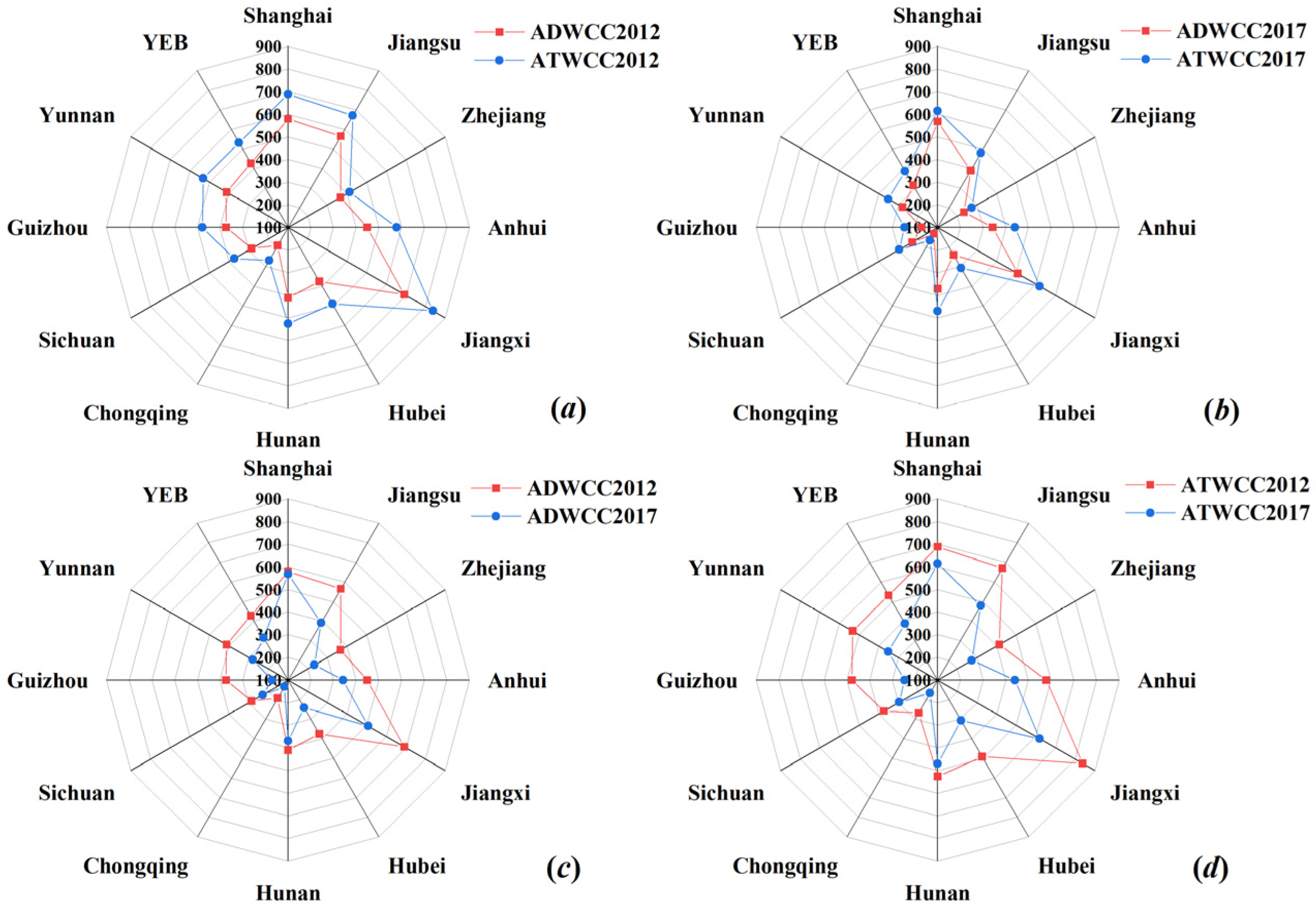
Figure 3.
Topologies of ATWCC in 11 provinces (cities) of YEB in (a) 2012 and (b) 2017.
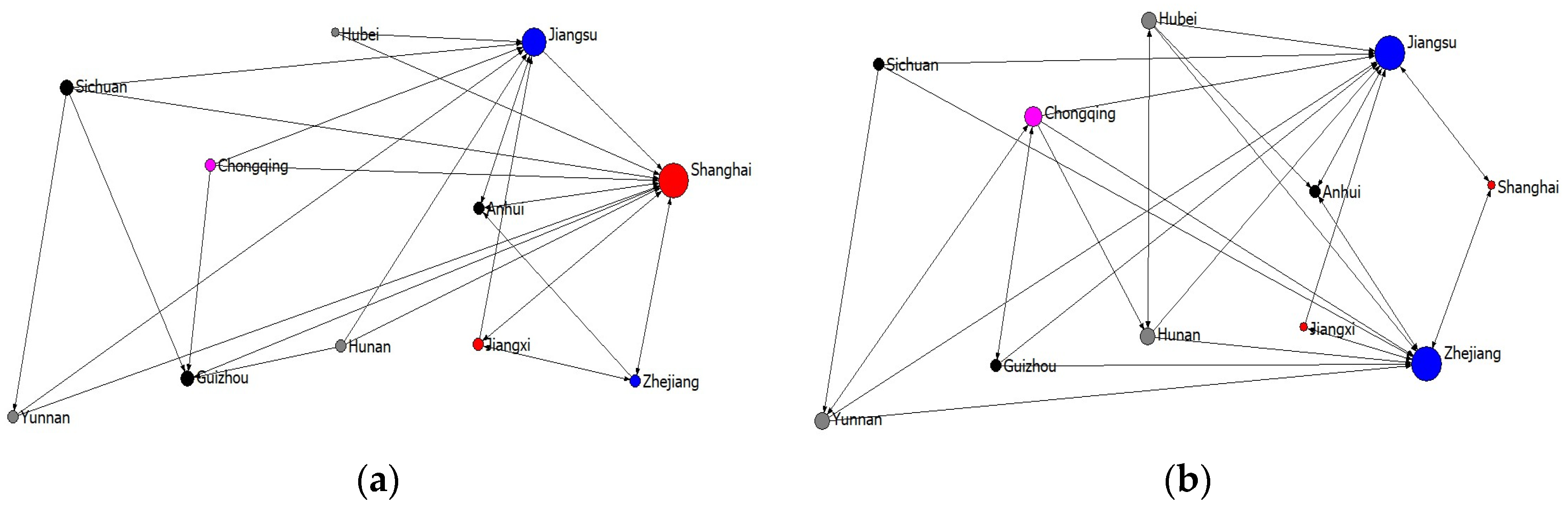
Figure 4.
Division of spatial correlation plates of ATWCC of YEB in (a) 2012 and (b) 2017.

Table 1.
Multi-regional input and output table of YEB.
| Intermediate Consumption | Final Consumption | Export | Total Output | |||||||||||||||
|---|---|---|---|---|---|---|---|---|---|---|---|---|---|---|---|---|---|---|
| Shanghai | … | Yunnan | China Outside YEB | Shanghai | … | Yunnan | China Outside YEB | |||||||||||
| S1 | … | Sn | … | S1 | … | Sn | S1 | … | Sn | |||||||||
| Intermediate input | Shanghai | S1 | … | … | … | … | … | … | … | |||||||||
| … | … | … | … | … | … | … | … | … | … | … | … | … | … | … | … | … | ||
| Sn | … | … | … | … | … | … | … | |||||||||||
| …… | …… | … | … | … | … | … | … | … | … | … | … | … | … | … | … | … | … | |
| Yunnan | S1 | … | … | … | … | … | … | … | ||||||||||
| … | … | … | … | … | … | … | … | … | … | … | … | … | … | … | … | … | ||
| Sn | … | … | … | … | … | … | … | |||||||||||
| China outside YEB | S1 | … | … | … | … | … | … | … | ||||||||||
| … | … | … | … | … | … | … | … | … | … | … | … | … | … | … | … | … | ||
| Sn | … | … | … | … | … | … | … | |||||||||||
| Import input | … | … | … | … | … | … | ||||||||||||
| Added value | … | … | … | … | … | … | ||||||||||||
| Total investment | … | … | … | … | … | … | ||||||||||||
| Water consumption | … | … | … | … | … | … | ||||||||||||
Table 2.
Classification of ATWCC plate attributes in the plate model.
| Proportion of Relationships within the Location | Proportion of Relationships Received by This Position | |
|---|---|---|
| Two-way overflow plate | Net benefit plate | |
| Net overflow plate | Broker plate | |
Table 3.
Overall characteristic indexes of spatial correlation network in 11 provinces (cities) of YEB in 2012 and 2017.
Table 3.
Overall characteristic indexes of spatial correlation network in 11 provinces (cities) of YEB in 2012 and 2017.
| Year | Network Relationship Number | Network Density | Network Correlation | Network Rank | Network Efficiency |
|---|---|---|---|---|---|
| 2012 | 28 | 0.255 | 1 | 0.773 | 0.711 |
| 2017 | 32 | 0.291 | 1 | 0.746 | 0.689 |
Table 4.
Structural central analysis of the spatial correlation network of ATWCC in 11 provinces (cities) of YEB in 2017.
Table 4.
Structural central analysis of the spatial correlation network of ATWCC in 11 provinces (cities) of YEB in 2017.
| Provinces (Cities) | PCD | CCD | ICD | |||||
|---|---|---|---|---|---|---|---|---|
| Point-Out Number | Point-In Number | Center Degree | Order | Center Degree | Order | Center Degree | Order | |
| Shanghai | 2 | 2 | 18.182 | 10 | 34.723 | 4 | 1.333 | 6 |
| Jiangsu | 2 | 9 | 81.818 | 1 | 52.304 | 2 | 7.333 | 3 |
| Zhejiang | 3 | 9 | 81.818 | 1 | 52.497 | 1 | 16.333 | 1 |
| Anhui | 2 | 3 | 27.273 | 7 | 36.357 | 3 | 1.333 | 6 |
| Jiangxi | 2 | 1 | 18.182 | 10 | 31.945 | 5 | 0.333 | 8 |
| Hubei | 4 | 1 | 36.364 | 4 | 16.969 | 11 | 0.333 | 8 |
| Hunan | 3 | 2 | 36.364 | 4 | 17.247 | 10 | 4 | 4 |
| Chongqing | 5 | 2 | 45.455 | 3 | 27.007 | 7 | 9 | 2 |
| Sichuan | 3 | 0 | 27.273 | 7 | 28.355 | 6 | 0 | 10 |
| Guizhou | 3 | 1 | 27.273 | 7 | 24.543 | 9 | 0 | 10 |
| Yunnan | 3 | 2 | 36.364 | 4 | 24.692 | 8 | 4 | 4 |
| Mean | 2.909 | 2.909 | 39.669 | 31.512 | 3.998 | |||
Table 5.
Division of spatial correlation plates of ATWCC in 11 provinces (cities) of YEB in 2017.
| Plate | Area | Number of Received Relationships | Number of Issued Relationships | Expected Internal Relationship Ratio (%) | Actual Internal Relationship Ratio (%) | ||
|---|---|---|---|---|---|---|---|
| Inside | Outside | Inside | Outside | ||||
| First plate | Zhejiang, Jiangsu | 0 | 18 | 0 | 5 | 10 | 0.000 |
| Second plate | Shanghai, Hunan, Jiangxi, Anhui. Hubei | 3 | 6 | 3 | 10 | 40 | 23.077 |
| Third plate | Chongqing, Sichuan, Guizhou. Yunnan | 5 | 0 | 5 | 9 | 30 | 35.714 |
Table 6.
Density matrix and image matrix of the spatial correlation plate of ATWCC in 11 provinces (cities) of YEB in 2017.
Table 6.
Density matrix and image matrix of the spatial correlation plate of ATWCC in 11 provinces (cities) of YEB in 2017.
| Plate | Density Matrix | Image Matrix | ||||
|---|---|---|---|---|---|---|
| First Plate | Second Plate | Third Plate | First Plate | Second Plate | Third Plate | |
| First plate | 0.000 | 0.500 | 0.000 | 0 | 1 | 0 |
| Second plate | 1.000 | 0.150 | 0.000 | 1 | 0 | 0 |
| Third plate | 1.000 | 0.050 | 0.417 | 1 | 0 | 1 |
Disclaimer/Publisher’s Note: The statements, opinions and data contained in all publications are solely those of the individual author(s) and contributor(s) and not of MDPI and/or the editor(s). MDPI and/or the editor(s) disclaim responsibility for any injury to people or property resulting from any ideas, methods, instructions or products referred to in the content. |
© 2023 by the authors. Licensee MDPI, Basel, Switzerland. This article is an open access article distributed under the terms and conditions of the Creative Commons Attribution (CC BY) license (https://creativecommons.org/licenses/by/4.0/).
Share and Cite
MDPI and ACS Style
Yang, Y.; Gao, Y.; Zhang, R.; Xu, J.; Yuan, H.; Wang, H. Agricultural Total Water Consumption Coefficient and Its Spatial Correlation Network in Yangtze River Economic Belt. Water 2023, 15, 2055. https://doi.org/10.3390/w15112055
AMA Style
Yang Y, Gao Y, Zhang R, Xu J, Yuan H, Wang H. Agricultural Total Water Consumption Coefficient and Its Spatial Correlation Network in Yangtze River Economic Belt. Water. 2023; 15(11):2055. https://doi.org/10.3390/w15112055
Chicago/Turabian StyleYang, Yafeng, Yuanyuan Gao, Ru Zhang, Jijun Xu, Haohan Yuan, and Hongrui Wang. 2023. "Agricultural Total Water Consumption Coefficient and Its Spatial Correlation Network in Yangtze River Economic Belt" Water 15, no. 11: 2055. https://doi.org/10.3390/w15112055
Note that from the first issue of 2016, this journal uses article numbers instead of page numbers. See further details here.