
Numerical Simulation of a Three-Stage Electrical Submersible Pump under Stall Conditions


1
National Research Center of Pumps, Jiangsu University, Zhenjiang 212013, China
2
School of Energy and Power Engineering, Jiangsu University, Zhenjiang 212013, China
3
Zhejiang Zhenxing Petrochemical Machinery Co., Ltd., Wenzhou 325204, China
4
Department of Agricultural and Biosystems Engineering, Alexandria University, Alexandria 21526, Egypt
*
Author to whom correspondence should be addressed.
Water 2023, 15(14), 2619; https://doi.org/10.3390/w15142619
Submission received: 8 June 2023
/
Revised: 13 July 2023
/
Accepted: 14 July 2023
/
Published: 19 July 2023
(This article belongs to the Special Issue Hydrodynamics in Pumping and Hydropower Systems)
Abstract
:This paper focuses on investigating the stall phenomenon of a three-stage electrical submersible pump using numerical methods by examining the internal and external characteristics of the pump under design conditions and critical stall and deep stall conditions. The energy losses inside the impeller and diffuser are also discussed. The internal flow at all pump stages under stall conditions is analyzed, highlighting differences and correlations. Under critical stall conditions, multiple vortices appear in the impeller channel of the first stage, while the flow in the secondary and final impeller remains smooth. Flow separation occurs in the diffusers at all three stages. Under deep stall conditions, the inlet setting angle causes all stages to enter a synchronous stall state. The range and intensity of vortices in the diffusers of all stages are further increased, seriously affecting the mainstream. This paper provides valuable insights for the research of internal flow and optimal design of electrical submersible pumps.
1. Introduction
Petroleum, as the primary fossil energy source, plays a crucial role in the development of modern society. With its advantages of high stability, high lift, and large displacement, the electrical submersible pump has become an important piece of equipment for artificial lifting and is widely used in high-yield wells and offshore oil production fields. In the process of petroleum development, the flow rate and pressure at the bottom of a well are constantly changing, and it is difficult to accurately estimate the actual production capacity of the oil well. As such, the electrical submersible pump needs to operate for long periods under conditions that deviate from the design parameters.
When an electrical submersible pump operates under low flow conditions, it is prone to stall. At low flow rates, the inlet angle of attack increases, leading to flow separation. As the stall develops, the flow separates and expands around the suction surface of the blades [1,2]. During stall conditions, the centrifugal pump’s flow head performance curve exhibits a positive slope, resulting in a saddle-shaped performance curve [3]. Additionally, the stall generates dynamic load on the impeller, which can result in vibration, fatigue, and even blade fracture at high-stress points [4,5,6]. The stall phenomenon not only reduces the pump efficiency but also has a severe negative impact on the safety and stability of the pump system [7,8].
In recent years, computational fluid dynamics (CFD) is increasingly employed in various engineering fields, particularly in the design and optimization of fluid machinery. Using CFD has dramatically improved the efficiency and accuracy of fluid machinery design and has become an essential tool in modern engineering [9,10]. The distribution of physical quantities, such as velocity and pressure inside the fluid machinery [11,12], can be obtained to identify the main energy losses and optimize the hydraulic performance of fluid machinery using CFD technology [13,14,15].
The performance characteristics of the pump under stall conditions have been studied by many authors. Wang et al. [16] studied a centrifugal pump with a diffuser and found that the rotational stall occurs in the diffuser when the flow rate is below 0.4 Qdes. At the same time, a positive slope segment appears on the performance curve. Pan et al. [17] investigated the external characteristic curve of a mixed-flow pump and observed a saddle-shaped curve. Their findings suggested that a vortex formed at the shroud of the pump, which reduced the effective outside diameter of the impeller outlet. Feng et al. [18] analyzed the internal flow pattern of a centrifugal pump under stall conditions and found that stall vortex frequently leads to the formation of a vortex at the outlet downstream. This phenomenon disrupts the flow pattern inside the pump and can cause a decrease in the pump’s head and efficiency. Li et al. [19] studied the impeller inlet prerotation in centrifugal pumps. Their research revealed that the presence of prerotation does not impact the occurrence of a positive slope in the external characteristic curve of the pump. However, prerotation may cause a sudden head drop, negatively affecting the pump performance. Hu et al. [20] conducted research on mixed-flow water jet propulsion pumps operating under low flow conditions. Their findings indicated that the presence of a diffuser did not impact the stall effect within the impeller.
Many authors have studied the internal flow characteristics of pumps under stall conditions. Fujisawa et al. [21] examined the progression of the rotational stall in a centrifugal compressor and observed that the separation flow on the hub side of the diffuser’s leading edge developed into a vortex with a tornado-like shape. JESE et al. [22] highlighted the importance of understanding the unsteady flow behavior in turbine pumps, particularly under stall conditions, to improve their performance and efficiency. Liu et al. [23] used Particle Image Velocity (PIV) technology to study the internal stall process of a two-blade centrifugal pump. As the flow rate decreases, flow separation occurs on the pressure surface of the blade and falls off to form a vortex. Li et al. [24] studied the stall conditions of a mixed-flow pump. They observed that when a rotary stall occurs, an unstable vortex occupies the inlet of the impeller. Miyabe et al. [25] studied a mixed-flow pump’s internal flow field under low flow conditions. Their results show that only one stall vortex is observed in the impeller when a rotating stall occurs. With a further reduction in the flow rate, the stall vortex develops into two. Ying et al. [26] conducted a numerical simulation of an electrical submersible pump under low flow conditions, and a region with large vortices in the current was formed at the leading edge and trailing edge of the first stage blade. Stel et al. [27] studied multi-stage electrical submersible pumps. Under 0.5 Qdes conditions, vortices in the impeller gathered at the suction surface, and the range and intensity of the vortices at all stages were slightly different.
Currently, research on pump stall conditions mostly focuses on single-stage pumps, whereas there is only minor research on multi-stage pumps with more complex structures and internal flow. In particular, there is a lack of systematic research on the differences between stages in the internal flow field of multi-stage pumps. This paper conducts a detailed analysis of multiple operating points in the saddle area of an electrical submersible pump, exploring the flow field and vortex distribution at all stages during stall conditions. The findings provide valuable insights for future research on the distinctions and relationships between multi-stage pumps.
2. Numerical Methods
2.1. Turbulence Model
Turbulence models are essential for achieving precise and efficient simulation results using the Reynolds-Averaged Navier–Stokes (RANS) equations. In the numerical simulation of fluid machinery, RANS together with an appropriate turbulence model is the most widely used method [28,29]. Currently, the two-equation turbulence models are most widely used in predicting the flow field characteristics of centrifugal pumps, namely, the standard k-ε model and k-ω model [30]. The two-equation models introduce two transport equations to calculate the eddy viscosity; they have shown good accuracy in predicting the pump flow field under design conditions [31,32].
The shear stress transport (SST) k-ω turbulence model proposed by Menter [33] in 1993 has been widely used in various flows and has demonstrated high accuracy in both the freestream and near-wall regions. The original k-ω model is retained near the wall, and the k-ε model is applied far away from the wall with the following turbulence coefficients.
The transport equations for k and ω are
The eddy viscosity of turbulent motion can be expressed as:
In the above equation, each constant is a mix of the internal constant and the external constant :
The expressions of the mixed function and other closed function equations are:
The constant values in the equation are shown in Table 1.
2.2. Entropy Production
According to the second law of thermodynamics, irreversible factors such as friction and unstable turbulence cause irreversible entropy production, which induces hydraulic losses in rotating machinery and then leads to energy dissipation and a decrease in efficiency. The entropy production distribution can be used to directly analyze the energy loss region of an electrical submersible pump and quantify the energy loss caused by unstable flow [34]. The entropy production inside an electrical submersible pump is mainly composed of three parts: velocity fluctuation, time-averaged velocity, and the wall effect [35]. The specific entropy production rate caused by velocity fluctuation, which is called the turbulent entropy production rate, is defined as follows:
In the SST k-ω turbulence model, the formula for calculating the turbulent entropy production rate can be written as follows [36]:
where ρ represents fluid density, kg/m3; ω represents the turbulent eddy frequency, s–1; k represents the turbulent energy, m2/s2; and T represents Kelvin temperature, 298.15 K.
The specific entropy production rate caused by time-averaged velocity, which is called the direct entropy production rate, is defined as follows:
where u, v, and w represent the three domains of velocity in a cartesian coordinate system, m/s.
In addition, the high-velocity gradient and pressure gradient on the blade surface of rotating fluid machinery cause a strong wall effect in the flow field, resulting in non-negligible irreversible flow losses. The entropy production rate in the tip region from the wall to the first layer of the grid can be calculated by [37]:
where indicates the shear stress in the wall (Pa); and indicates the velocity of the first grid near the wall (m/s).
Therefore, the total entropy production () can be obtained through the volume integral of the local entropy production rate and the surface integral of the wall entropy production rate:
Based on the entropy production theory, the total entropy production power can be written as:
where represents direct entropy production power; represents turbulent entropy production power; and represents wall entropy production power.
2.3. Computational Model
This study investigated the design and performance of a specific type of electrical submersible pump commonly used in the oil and gas industry for pumping fluids from deep wells. The pump was designed to operate under specific working conditions, including a flow rate of Qdes = 104.2 m3/h, the single-stage head Hdes = 8 m, rated speed ndes = 2900 r/min, and the specific speed ns = 375. To model the pump’s performance and behavior, the UG NX10.0 software was used to create a computational model of the pump’s calculation area, as shown in Figure 1. The model used a closed impeller design and consisted of detailed geometric parameters for the impeller and diffuser of the pump, as provided in Table 2.
2.4. Mesh and Boundary Condition
The steady numerical simulation of the electrical submersible pump involved meshing the inlet, front chamber, impeller, and diffuser through ICEM. To ensure the accuracy of the simulation, the SST k-ω turbulence model is selected and the convergence residual is set to 10−5. The interface between the stationary and rotational domain is selected as the frozen rotor in the steady state simulation, while the transient rotor stator is used in the transient simulation. In the transient simulation, the time step is set to the time taken for the impeller to rotate 5°, which is 2.8736 × 10⁻⁴ s. The rotor stator interfaces adopt the frozen rotor mode. Due to the complex flow and large pressure gradient near the blade wall, the mesh near the impeller blade and diffuser vane are encrypted to ensure the accuracy of numerical simulation. The SST k-ω turbulence model gives the most accurate results when y+ is less than 5, and the accuracy is also excellent when y+ is less than 100 [38]. The y+ values in the impeller domain are kept at less than 100 to meet the SST k-ω turbulence model requirements. The distribution of y+ values near the blades is shown in Figure 2. To minimize the impact of boundary conditions on the simulation results, the inlet section is set to 5 times the pipe diameter, and the outlet section is set to 10 times the pipe diameter. The fluid medium used in the simulation is clear water at a temperature of 25 °C. The boundary conditions are set to pressure inlet and mass flow outlet, while the wall boundary condition is set to the no-slip wall and automatic wall function.
To ensure the accuracy and efficiency of the numerical calculations reported in this paper, selecting a mesh size that does not significantly affect the simulation accuracy is essential. To verify the mesh independence of the results, eight different mesh sizes were selected and tested, as shown in Figure 3. The results indicated that the head values became increasingly stable as the number of meshes increased. Based on these findings, a mesh size of 8,237,945 was chosen for the numerical calculations to ensure accuracy and efficiency.
3. Results and Discussions
3.1. External Characteristics Comparison
To verify the accuracy of the numerical calculations, external characteristics testing was conducted on a physical model of a three-stage electrical submersible pump. The testing was carried out using appropriate testing equipment, as shown in Figure 4, which included a ZNX-AK flow meter (Siemens; Shanghai, China) with a measuring accuracy of ±0.1% and an SGDN torque meter (Siemens; Shanghai, China) with a measuring accuracy of ±0.5%. To ensure the dimensional accuracy of the model, the impeller and diffuser were constructed using finely cast stainless steel material.
Figure 5 presents the head, efficiency, and power performance curves of the electrical submersible pump. As the numerical calculation neglects some mechanical losses during the testing process, the simulated head and efficiency values are higher than the test values, while the simulated power values are lower than the test values. However, the slight difference between the numerical calculation results and the test values indicates that the numerical calculation is accurate and reliable. Furthermore, when the internal stall of the electrical submersible pump occurs, the external characteristic performance curve changes, resulting in instability that is depicted as a positive slope curve in this model. This paper defines the highest point before the head drop as the critical stall point, the lowest point before the head rise as the deep stall point, and the highest efficiency point as the design point. Based on the observations in Figure 5, it is evident that the saddle area of the electrical submersible pump occurs at 0.88 Qdes for the critical stall and at 0.66 Qdes for the deep stall.
The hydraulic performance of each stage in the three-stage electrical submersible pump is analyzed in the following section. To simplify the expression, the three stages are referred to as Stage 1, Stage 2, and Stage 3. The impellers are referred to as impeller 1, impeller 2, and impeller 3. As shown in Figure 6, Ha represents the average head of a single stage, H1 represents the difference in head between the inlet of the stage 1 impeller and the outlet of the diffuser, and H2 and H3 represent the head of stage 2 and stage 3, respectively. The head of stage 1 is higher than that of the other two stages, and the head of a single stage gradually decreases as the number of stages increases. The heads created by the different stages of a multistage pump may not be identical (even if the impellers and diffusers have the same geometry). This is because the boundary conditions change as the fluid flows out of stage 1 and passes through the diffuser. Therefore, each stage affects the other and changes the overall hydraulic performance of the pump.
3.2. Analysis of Flow Field under Design Conditions
Figure 7 illustrates the streamline and low-speed zone distribution of the electrical submersible pump under design conditions. Based on comprehensive considerations, the velocity values are constrained between a minimum of 1 m/s and a maximum of 15 m/s. The yellow area in Figure 7 represents the low-speed zone of 1 m/s in the electrical submersible pump. The flow field inside the impeller channel is smooth, with a small wake resulting from the inherent secondary flow in the impeller 1 channel, which accumulates at the impeller outlet. When the absolute vorticity experiences streamline curvature or the Coriolis force, it generates the flow direction component of vorticity, leading to inherent secondary flow [39]. Simultaneously, the inherent secondary flow generates a force that moves the fluid with lower kinetic energy towards a relatively stable area of low static pressure. Within the impeller flow channel, the inherent secondary flow flows from the hub towards the shroud and the pressure surface towards the suction surface [40]. Thus, the low kinetic energy fluid region in the impeller is concentrated at the intersection of the suction surface and the shroud. Under design conditions, flow separation occurs at 70% of the blade chord length of impeller 1, forming vortex A and spiral vortex B. At the outlet of the flow channel, a small amount of leakage flow from the upper blade brings high kinetic energy fluid to vortex B, which causes it to dissipate. The location of the vortex structure position is relatively stable and does not affect the core region of the flow. Due to the changes in the inlet boundary conditions, the impeller 2 and impeller 3 flow paths do not exhibit significant flow separation. At each stage, the flow separation occurs at the exit of the diffuser, and the low-speed zone primarily accumulates in the middle of the runner’s exit and close to the hub.
Based on the previous analysis, it is apparent that the inner vortex of the impeller is mainly distributed near the shroud, whereas the vortex in the diffuser is distributed near the hub. Therefore, the velocity distribution of five different blade-to-blade surfaces is further analyzed and their locations are shown in Figure 8a. As per Figure 8b,c it is evident that there exist some low-velocity fluids near the pressure surface of the blade, which results from circumferential vortices caused by the inherent secondary flow directed from the pressure surface to the suction surface. The low-velocity region at the shroud and outlet of the impeller suction surface is responsible for the development of induced vortex B. Figure 8e,f shows that vortex B and the leakage vortex have particular impacts on the outlet of the flow channel. With flow deceleration in the diffuser, most of the fluid’s kinetic energy is transformed into potential pressure energy.
3.3. Analysis of Flow Field under Critical Stall Conditions
Figure 9 reveals that as the flow rate decreases, the velocity values of each section decrease under the critical stall conditions, and the vortex coverage increases. The fluid’s kinetic energy in the impeller 1 flow channel decreases, causing the vortex to grow and move towards the middle of the flow channel. The vortex ranges in impeller 2 and impeller 3 are smaller than that of the primary impeller. The fluid’s kinetic energy near the suction surface is further reduced, allowing the liquid to flow again under the reverse pressure gradient, forming vortex B. Vortex C emerges directly below vortex A and differentiates into vortex D at the exit. The flow field in the impeller 2 and impeller 3 channels remains stable. Similar to the design conditions, the vortices in the diffuser gather near the outlet of the flow channel and the hub.
In Figure 10, the vortex structure inside the electrical submersible pump is highlighted through the yellow circle. As shown in Figure 10a,b, as the flow rate decreases, the inlet impeller angle increases, causing a low-speed zone to appear at the leading edge of the blade and promoting flow separation. At the same time, the range and intensity of the vortex on the suction surface of the blade increase. In contrast, the velocity on the impeller 2 and impeller 3 surfaces decreases, but there is no significant flow separation on the suction surface of the blade. Flow separation near the diffuser hub occurs at all stages, with the vortex impacting the outlet flow field. This is due to the conversion of most of the kinetic energy of the fluid into pressure potential energy by the diffuser, resulting in low kinetic energy of the fluid near the outlet of the diffuser. The intensity of the vortex in the diffuser increases with the number of stages. As shown in Figure 10d,e, the fluid kinetic energy at the entrance of impeller 1 is relatively high, which suppresses the occurrence of flow separation. As the kinetic energy of the fluid weakens, flow separation occurs in the middle of the flow channel, forming a separation vortex. Near the outlet of the impeller, the separation vortex migrates towards the pressure surface under the impact of a small amount of leakage flow from adjacent channels. After the fluid passes through the diffuser, the angle of attack of the impeller 2 and impeller 3 blades decreases, resulting in no apparent flow separation.
3.4. Analysis of Flow Field under Deep Stall Conditions
As shown in Figure 11, under the conditions of a deep stall, the inlet vortices within impeller 1 cause severe blockage to the flow passage. Large-scale return flow vortices exist inside impeller 1 and are accompanied by strong interchannel overflow phenomena. The internal stall phenomenon also occurs in impellers 2 and 3 of the electrical submersible pump, and the morphology of the vortex is similar to that of impeller 1. Strong vorticity is found near the outlet of the diffuser channels which influences the flow field at the inlet to the subsequent stage. The sudden drop in the head of the electrical submersible pump is mainly due to the severe stall of the impeller and diffuser.
Under the conditions of a deep stall, the flow field at each section becomes more non-uniform, as depicted in Figure 12. The suction surface of blades at all stages has extensive ranges of vortices, which enhance the development of channel vortices. The high angle of attack leads to further advancement of flow separation in the diffuser, and the stall vortex occupies the entire flow passage. Figure 12a–c reveal that the vortex intensity in the diffuser gradually weakens from the hub to the shroud. In Figure 12d,e, the flow channels of impellers at all stages are occupied by vortices. The backflow at the inlet of impeller 1 is severe, and the flow field at the inlet of impeller 2 and impeller 3 is asymmetric, with different vortex positions and sizes.
3.5. Vortex Evolution Process in the Impeller and Diffuser under Stall Conditions
Figure 13 shows the evolution process of vortices in the impeller and diffuser during T (T = 0.02069 s) time under critical stall conditions. At T0, the inner channel of impeller 1 contains vortex A near the outlet and vortex B in the middle of the flow channel. At 0.25T, vortex A disappears, and vortex B migrates towards the outlet, shedding at the front edge of the suction force to form vortex C. At 0.5T, the energy of vortex B weakens and further migrates towards the outlet, while the intensity of vortex C increases and moves towards the middle of the flow channel. At 0.75T, the high kinetic energy fluid brought by the leakage flow rapidly dissipates vortex B, and vortex C migrates to the middle of the flow channel. At moment T, vortex C tends to collapse and disappear, and the flow separation at the leading edge of the blade generates vortex D. The internal vortices of impellers 2 and 3 do not exhibit obvious evolution patterns.
Figure 14 shows the evolution process of vortices in the impeller and diffuser under deep stall conditions within 0.67T. Channels 1, 2 and 3 represent three different channels in the impeller 1. The evolution process of vortex structure in impeller 1 was marked by yellow circle. By comparing channels 2 and 3 of impeller 1, it can be found that there are differences in the evolution law and range of vortices within different channels. The symmetry of the inlet flow field of impellers 2 and 3 disappears. The flow separation in the diffuser starts at the leading edge of the guide vanes, and the vortices develop and grow inside the channel, causing a serious impact on the outlet.
3.6. Energy Loss Analysis
The entropy production power loss inside the impeller and diffuser of the electrical submersible pump was obtained through steady simulation, as shown in Figure 15. (turbulent entropy production power) inside the impeller and diffuser is the main component of (total entropy production power), while (wall entropy production power) and (direct entropy production power) account for a small proportion of . The entropy production power loss inside the impeller increases with the increase in stages, and the power loss inside the diffuser is the same in each stage. As a stall occurs, the energy loss caused by internal vortices in the impeller and diffuser increases.
4. Conclusions
In this paper, numerical simulations of electrical submersible pumps are investigated and their internal characteristics are analyzed under design, critical stall, and deep stall operating conditions. Based on the analysis results, the following conclusions can be drawn:
- (1)
- Under critical stall conditions, impeller 1 generates inlet and multiple channel vortices, which when combined with inherent secondary flow and wake, result in turbulence within the impeller’s flow field. The internal vortex evolution period of impeller 1 is approximately 0.75T; however, the scale of internal vortices in impellers 2 and 3 is small with no apparent evolution period.
- (2)
- Under deep stall conditions, large-scale vortex structures manifest within all stages of the impeller, resulting in severe channel blockage. Flow separation commences at the leading edge of the guide vanes in the diffuser, with vortices developing and expanding inside the channel to cause a significant impact on outlet performance. The scales and evolution patterns of these vortices vary across different channels within impeller 1.
- (3)
- The turbulent entropy production power within the impeller and diffuser constitutes the primary component of total entropy production power. The entropy production power loss inside the impeller increases with the increase in stages, and the power loss inside the diffuser is the same in each stage. Under deep stall conditions, frequent vortex shedding inside these components results in significant energy loss.
Author Contributions
Conceptualization, Y.W. and L.B.; methodology, Z.W.; software, Y.W.; validation, X.S., M.A.E.-E. and L.Z.; formal analysis, Y.W.; investigation, Z.W.; resources, X.S.; data curation, L.B.; writing—original draft preparation, Y.W.; writing—review and editing, L.B. and M.A.E.-E.; visualization, M.A.E.-E.; supervision, L.B.; project administration, L.Z.; funding acquisition, L.B. All authors have read and agreed to the published version of the manuscript.
Funding
This work was supported by the “Pioneer” and “Leading Goose” R&D Program of Zhejiang (2022C03170), the High-tech Key Laboratory of Agricultural Equipment and Intelligence of Jiangsu Province (Grant No. MAET202121), the National Natural Science Foundation of China (Grant Nos. 52079058 and 52209113) and the Nature Science Foundation of Jiangsu Province (Grant No. BK20220544).
Data Availability Statement
The data presented in this article are available upon request from the corresponding author.
Conflicts of Interest
The authors declare no conflict of interest.
References
- Jese, U.; Fortes-Patella, R.; Antheaume, S. High head pump-turbine: Pumping mode numerical simulations with a cavitation model for off-design conditions. IOP Conf. Ser.-Earth Environ. Sci. 2014, 22, 032048. [Google Scholar] [CrossRef]
- Jese, U.; Fortes-Patella, R. Unsteady numerical analysis of the rotating stall in pump-turbine geometry. IOP Conf. Ser.-Earth Environ. Sci. 2016, 49, 042005. [Google Scholar] [CrossRef]
- Day, I. Stall, Surge, and 75 Years of Research. J. Turbomach. 2015, 138, 011001. [Google Scholar] [CrossRef]
- Liu, T.; Zhang, Y.; Du, X. A review of rotating stall of pump turbines. J. Hydroelectr. Eng. 2015, 34, 16–24. [Google Scholar]
- Yang, J.; Yuan, S.; Pei, J.; Zhang, J. Overview of rotating stall in centrifugal pumps with vaned diffuser. J. Drain. Irrig. Mach. Eng. 2015, 33, 369–373. [Google Scholar]
- Zhang, N.; Yang, M.; Li, Z.; Sun, X. Pressure pulsation of centrifugal pump with tilt volute. J. Mech. Eng. 2012, 48, 164–168. [Google Scholar] [CrossRef]
- Ullum, U.; Wright, J.; Dayi, O.; Ecder, A.; Soulaimani, A.; Piché, R.; Kamath, H. Prediction of rotating stall within an impeller of a centrifugal pump based on spectral analysis of pressure and velocity data. J. Phys. Conf. Ser. 2006, 52, 36–45. [Google Scholar] [CrossRef]
- Li, W.; Ping, Y.; Shi, W. Research progress in rotating stall in mixed-flow pumps with guide vane. J. Drain. Irrig. Mach. Eng. 2019, 37, 737–745. [Google Scholar]
- Zhou, L.; Bai, L.; Li, W.; Shi, W.; Wang, C. PIV validation of different turbulence models used for numerical simulation of a centrifugal pump diffuser. Eng. Comput. 2018, 35, 2–17. [Google Scholar] [CrossRef]
- Yang, Y. Interstage difference of pressure pulsation in a three-stage electrical submersible pump. J. Pet. Sci. Eng. 2021, 196, 107653. [Google Scholar] [CrossRef]
- Goto, A. Study of internal flows in a mixed-flow pump impeller at various tip clearances using three-dimensional viscous flow computations. J. Turbomach. 1992, 114, 373–382. [Google Scholar] [CrossRef]
- Goto, A. The effect of tip leakage flow on part-load performance of a mixed-flow pump impeller. J. Turbomach. 1992, 114, 383–391. [Google Scholar] [CrossRef]
- Wang, F. Research progress of computational model for rotating turbulent flow in fluid machinery. Trans. Chin. Soc. Agric. Mach. 2016, 47, 1–14. [Google Scholar]
- El-Emam, M.A.; Zhou, L.; Yasser, E.; Bai, L.; Shi, W. Computational methods of erosion wear in centrifugal pump: A state-of-the-art review. Arch. Comput. Methods Eng. 2022, 29, 3789–3814. [Google Scholar] [CrossRef]
- Hang, J.; Bai, L.; Zhou, L.; Jiang, L.; Shi, W.; Agarwal, R. Inter-stage energy characteristics of electrical submersible pump under gassy conditions. J. Energy 2022, 256, 124624. [Google Scholar] [CrossRef]
- Hong, W.; Hiroshi, T. Experimental and numerical study of unsteady flow in a diffuser pump at off-design conditions. J. Fluids Eng. 2003, 125, 767–778. [Google Scholar]
- Pan, Z.; Li, J.; Li, X.; Yuan, S. Curve instability and rotating stall. Trans. Chin. Soc. Agric. Mach. 2012, 43, 64–68. [Google Scholar]
- Feng, J.; Wang, C.; Luo, X. Rotating stall in centrifugal pump impellers under part-load conditions. J. Hydroelectr. Eng. 2018, 37, 117–124. [Google Scholar]
- Li, X.; Yuan, S.; Pan, Z.; Li, Y.; Liu, W. Dynamic characteristics of rotating stall in mixed flow pump. J. Appl. Math. 2013, 2013, 4819–4828. [Google Scholar] [CrossRef] [Green Version]
- Hu, F.; Wu, P.; Wu, D.; Wang, L. Numerical study on the stall behavior of a water jet mixed-flow pump (Article). J. Mar. Sci. Technol. 2014, 19, 438–449. [Google Scholar]
- Fujisawa, N.; Inui, T.; Ohta, Y. Evolution process of diffuser stall in a centrifugal compressor with vaned diffuser. J. Turbomach. 2019, 141, 41009. [Google Scholar] [CrossRef]
- Jese, U.; Skotak, A.; Mikulasek, J. Cavitating vortices in the guide vanes region related to the pump-turbine pumping mode rotating stall. J. Phys. Conf. Ser. 2017, 813, 12043. [Google Scholar] [CrossRef]
- Hou-Lin, L.U.; Dong-Sheng, Y.A.N.G.; Ming-Gao, T.A.N.; Kai, W.A.N.G.; Su-Guo, Z.H.U.A.N.G.; Hui, D.U. 3D-PIV measurements of stall in double blade centrifugal pump. J. Shanghai Jiaotong Univ. 2012, 46, 734–739. [Google Scholar]
- Li, Y.; Li, R.; Wang, X.; Zhao, W.; Li, P. Numerical simulation of unstable characteristics in head curve of mixed-flow Pump. J. Drain. Irrig. Mach. Eng. 2013, 31, 6. [Google Scholar]
- Miyabe, M.; Maeda, H.; Umeki, I.; Jittani, Y. Unstable head-flow characteristic generation mechanism of a low specific speed mixed flow pump. J. Therm. Sci. 2006, 15, 115–120. [Google Scholar] [CrossRef]
- Ying, G. Numerical Analysis of Flow Field of Electrical Submersible Pump; Zhejiang University: Zhejiang, China, 2004. [Google Scholar]
- Stel, H.; Sirino, T.; Ponce, F.J.; Chiva, S.; Morales, R.E.M. Numerical investigation of the flow in a multi-stage electric submersible pump (Article). J. Pet. Sci. Eng. 2015, 136, 41–54. [Google Scholar] [CrossRef]
- Li, W.; Zhou, L.; Shi, W.D.; Ji, L.; Yang, Y.; Zhao, X. PIV experiment of the unsteady flow field in mixed-flow pump under part loading condition. Exp. Therm. Fluid Sci. 2017, 83, 191–199. [Google Scholar] [CrossRef]
- Tuzson, J. Centrifugal Pump Design; John Wiley and Sons: New York, NY, USA, 2000. [Google Scholar]
- Chen, Q. Predictive Performance of Several Turbulence Models in Turbomachinery Related Flows; Tsinghua University: Beijing, China, 2007. [Google Scholar]
- Bai, L.; Yang, Y.; Zhou, L.; Li, Y.; Xiao, Y.; Shi, W. Optimal design and performance improvement of an electric submersible pump impeller based on Taguchi approach. Energy 2022, 252, 124032. [Google Scholar] [CrossRef]
- Han, Y.; Zhou, L.; Bai, L.; Shi, W.; Agarwal, R. Comparison and validation of various turbulence models for U-bend flow with a magnetic resonance velocimetry experiment. Phys. Fluids 2021, 33, 125117. [Google Scholar] [CrossRef]
- Menter, F.R.; Kuntz, M.; Langtry, R. Ten years of industrial experience with the SST turbulence model. Turbul. Heat Mass Transf. 2003, 4, 625–632. [Google Scholar]
- Sun, L.; Pan, Q.; Zhang, D.; Zhao, R.; van Esch, B.B. Numerical study of the energy loss in the bulb tubular pump system focusing on the off-design conditions based on combined energy analysis methods. Energy. 2022, 258, 124794. [Google Scholar] [CrossRef]
- Wang, X.; Wang, Y.; Liu, H.; Xiao, Y.; Jiang, L.; Li, M. A numerical investigation on energy characteristics of centrifugal pump for cavitation flow using entropy production theory. Int. J. Heat Mass Transfer. 2023, 201, 123591. [Google Scholar] [CrossRef]
- Kock, F.; Herwig, H. Entropy production calculation for turbulent shear flows and their implementation in cfd codes. Int. J. Heat Fluid Flow 2005, 26, 672–680. [Google Scholar] [CrossRef]
- Zhou, L.; Hang, J.; Bai, L.; Krzemianowski, Z.; El-Emam, M.A.; Yasser, E.; Agarwal, R. Application of entropy production theory for energy losses and other investigation in pumps and turbines: A review. Appl. Energy 2022, 318, 119211. [Google Scholar] [CrossRef]
- Tao, R.; Xiao, R.; Wang, F.; Liu, W. Improving the cavitation inception performance of a reversible pumpturbine in pump mode by blade profile redesign: Design concept, method and applications. Renew. Energy 2019, 133, 325–342. [Google Scholar] [CrossRef]
- Cai, Z.; Luo, S. Secondary flow and wake development in fluid machinery impeller. J. Huazhong Univ. Sci. Technol Nat. Sci. Ed. 2001, 29, 4. [Google Scholar]
- Wang, C.; Wang, F.; An, D.; Yao, Z.; Xiao, R.; Lu, L.; He, C.; Zou, Z. A general alternate loading technique and its applications in the inverse designs of centrifugal and mixed-flow pump impellers. Sci. China (Technol. Sci.) 2021, 64, 898–918. [Google Scholar] [CrossRef]
Figure 1.
Numerical simulation model. (a) Calculation domain of electrical submersible pump. (b) 2D illustration of the ESP stage.
Figure 1.
Numerical simulation model. (a) Calculation domain of electrical submersible pump. (b) 2D illustration of the ESP stage.
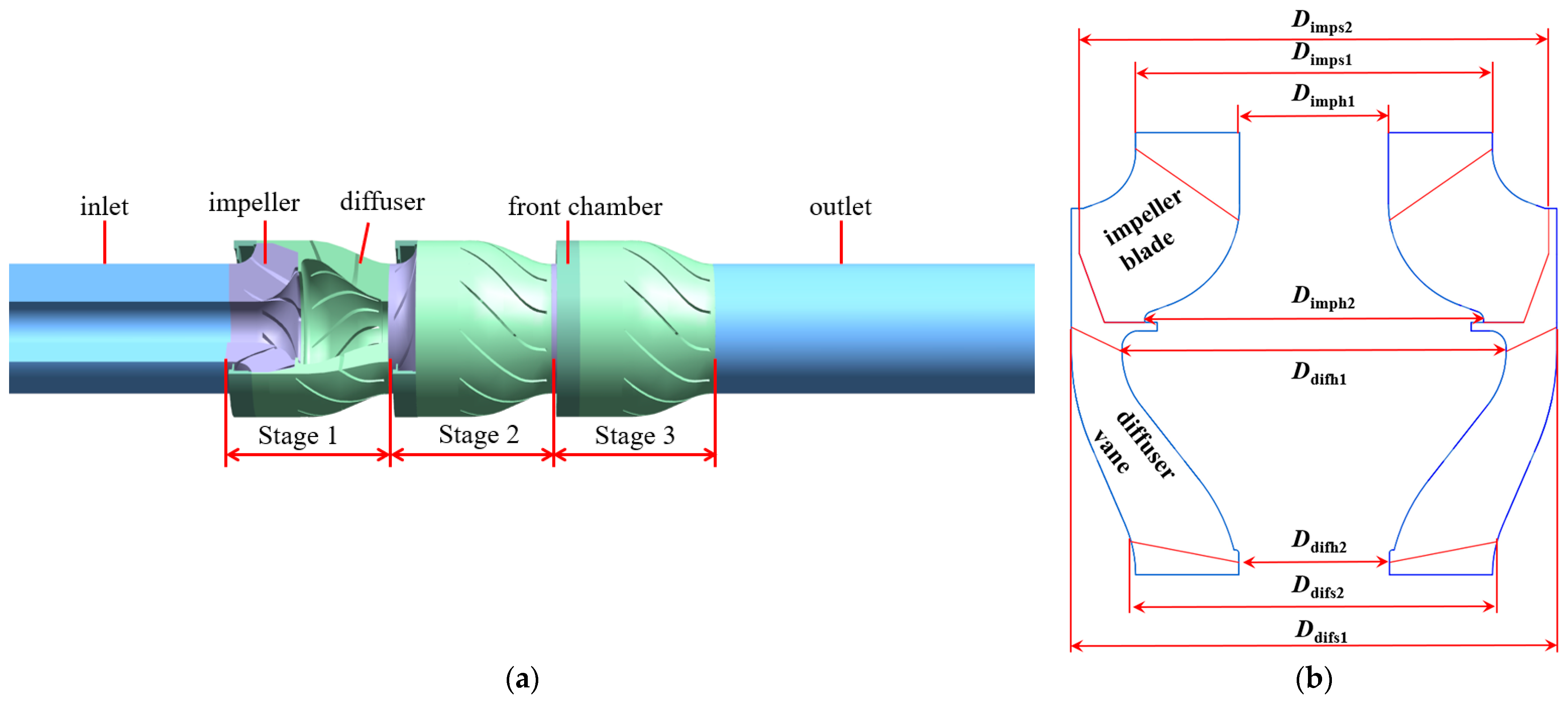
Figure 2.
Y+ distribution on the blade surface.

Figure 3.
Mesh independence of solution analysis.
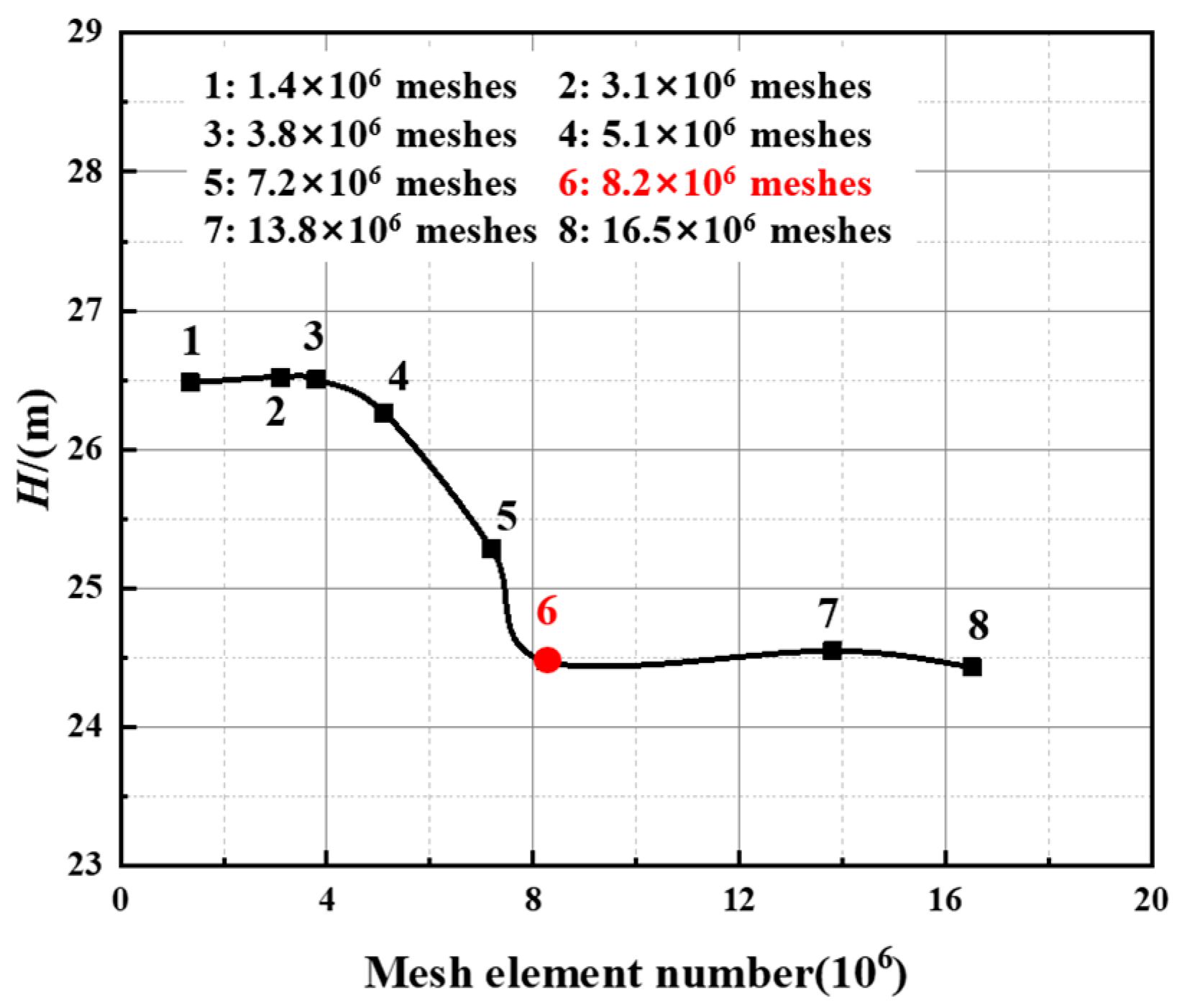
Figure 4.
Testing equipment.

Figure 5.
Comparison between test and simulation of the external characteristic curve.
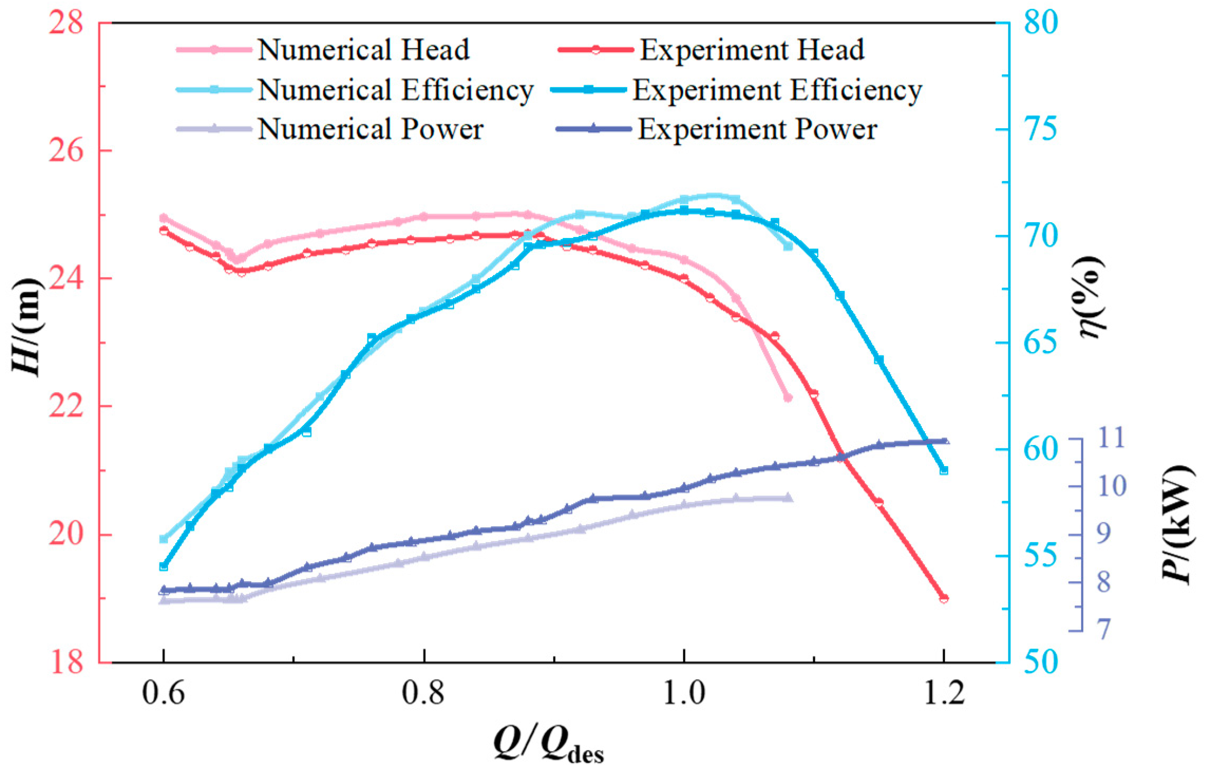
Figure 6.
Head diagram of each stage.
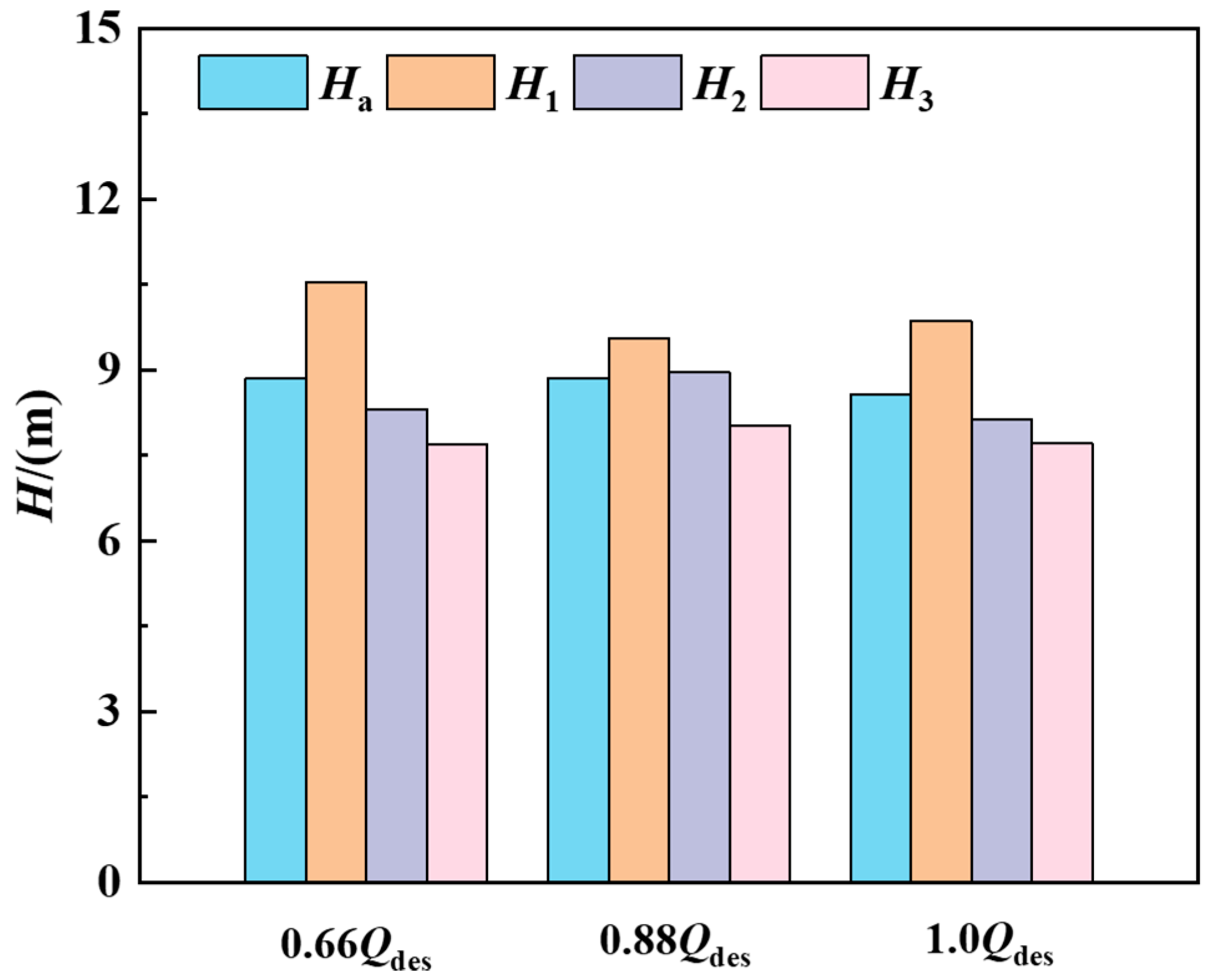
Figure 7.
Velocity streamlines and low-speed zone distribution diagram under design conditions.
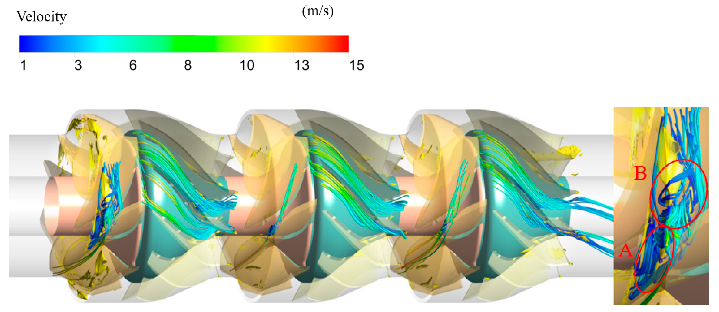
Figure 8.
Streamline and velocity distributions on different span surfaces under design conditions. (a) Schematic diagram of different blade-to-blade surfaces. (b) 0.1 Span. (c) 0.2 Span. (d) 0.5 Span. (e) 0.8 Span. (f) 0.9 Span.
Figure 8.
Streamline and velocity distributions on different span surfaces under design conditions. (a) Schematic diagram of different blade-to-blade surfaces. (b) 0.1 Span. (c) 0.2 Span. (d) 0.5 Span. (e) 0.8 Span. (f) 0.9 Span.

Figure 9.
Velocity streamlines and low-speed zone distribution diagram under critical stall conditions.
Figure 9.
Velocity streamlines and low-speed zone distribution diagram under critical stall conditions.
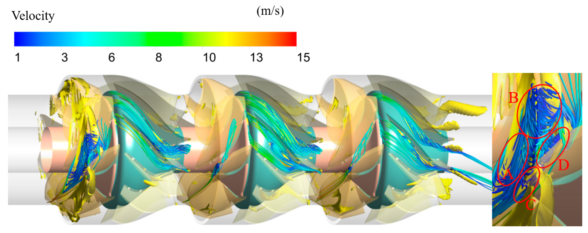
Figure 10.
Streamline and velocity distributions on different span surfaces under critical stall conditions. (a) 0.1 Span. (b) 0.2 Span. (c) 0.5 Span. (d) 0.8 Span. (e) 0.9 Span.
Figure 10.
Streamline and velocity distributions on different span surfaces under critical stall conditions. (a) 0.1 Span. (b) 0.2 Span. (c) 0.5 Span. (d) 0.8 Span. (e) 0.9 Span.
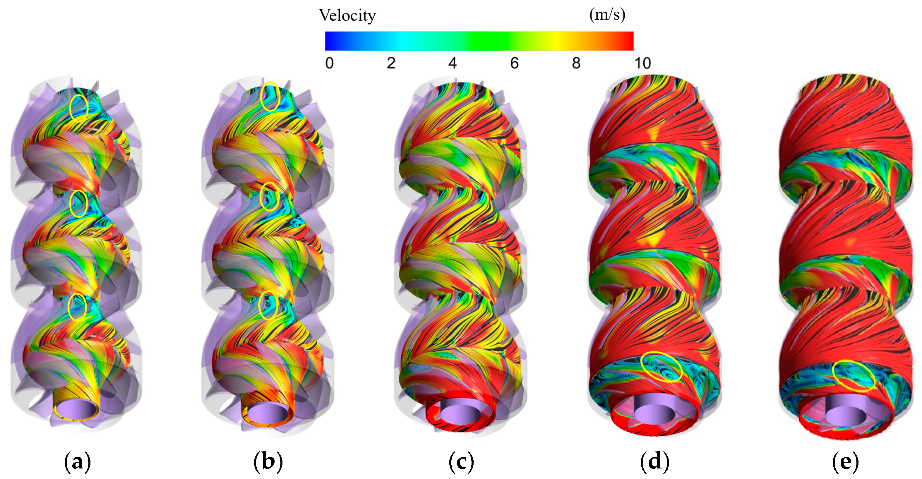
Figure 11.
Velocity streamlines and low-speed zone distribution diagram under deep stall conditions.
Figure 11.
Velocity streamlines and low-speed zone distribution diagram under deep stall conditions.

Figure 12.
Streamline and velocity distributions on different span surfaces under deep stall conditions. (a) 0.1 Span. (b) 0.2 Span. (c) 0.5 Span. (d) 0.8 Span. (e) 0.9 Span.
Figure 12.
Streamline and velocity distributions on different span surfaces under deep stall conditions. (a) 0.1 Span. (b) 0.2 Span. (c) 0.5 Span. (d) 0.8 Span. (e) 0.9 Span.

Figure 13.
Vortex evolution process in the impeller and the diffuser under critical stall conditions. (a) 0.9 Span of the impeller and 0.2 Span of the diffuser. (b) 0.5 Span of impeller and diffuser.
Figure 13.
Vortex evolution process in the impeller and the diffuser under critical stall conditions. (a) 0.9 Span of the impeller and 0.2 Span of the diffuser. (b) 0.5 Span of impeller and diffuser.

Figure 14.
Vortex evolution process in the impeller and the diffuser under deep stall conditions. (a) 0.9 Span of the impeller and 0.2 Span of the diffuser. (b) 0.5 Span of impeller and diffuser.
Figure 14.
Vortex evolution process in the impeller and the diffuser under deep stall conditions. (a) 0.9 Span of the impeller and 0.2 Span of the diffuser. (b) 0.5 Span of impeller and diffuser.

Figure 15.
Power loss of impeller and diffusers. (a) Total entropy production power. (b) Turbulent entropy production power. (c) Wall entropy production power. (d) Direct entropy production power.
Figure 15.
Power loss of impeller and diffusers. (a) Total entropy production power. (b) Turbulent entropy production power. (c) Wall entropy production power. (d) Direct entropy production power.


Table 1.
Constants of the SST k-ω model.
| Constants | Value |
|---|---|
| 0.31 | |
| 5/9 | |
| 0.44 | |
| 3/40 | |
| 0.0828 | |
| 9/100 | |
| 0.85 | |
| 1 | |
| 0.5 | |
| 0.856 |
Table 2.
Model geometry parameters.
| Impeller Hydraulic Geometry Parameters | Hydraulic Geometry Parameters of Diffuser | ||
|---|---|---|---|
| Inlet inner diameter Dimph1/mm | 36 | Inlet inner diameter Ddifh1/mm | 76 |
| Inlet outer diameter Dimps1/mm | 86.5 | Inlet outer diameter Ddifs1/mm | 117.5 |
| Outlet inner diameter Dimph2/mm | 82 | Outlet inner diameter Ddifh2/mm | 36.5 |
| Outlet outer diameter Dimps2/mm | 113.5 | Outlet outer diameter Ddifs2/mm | 86.5 |
| Number of blades Zimp/vanes | 7 | Number of blades Zdif/ vanes | 11 |
| Inlet blade angle βimp1/° | 25 | Inlet blade angle βdif1/° | 55 |
| Outlet blade angle βimp2/° | 36 | Outlet blade angle βdif2/° | 87 |
Disclaimer/Publisher’s Note: The statements, opinions and data contained in all publications are solely those of the individual author(s) and contributor(s) and not of MDPI and/or the editor(s). MDPI and/or the editor(s) disclaim responsibility for any injury to people or property resulting from any ideas, methods, instructions or products referred to in the content. |
© 2023 by the authors. Licensee MDPI, Basel, Switzerland. This article is an open access article distributed under the terms and conditions of the Creative Commons Attribution (CC BY) license (https://creativecommons.org/licenses/by/4.0/).
Share and Cite
MDPI and ACS Style
Wang, Y.; Wang, Z.; Song, X.; Bai, L.; El-Emam, M.A.; Zhou, L. Numerical Simulation of a Three-Stage Electrical Submersible Pump under Stall Conditions. Water 2023, 15, 2619. https://doi.org/10.3390/w15142619
AMA Style
Wang Y, Wang Z, Song X, Bai L, El-Emam MA, Zhou L. Numerical Simulation of a Three-Stage Electrical Submersible Pump under Stall Conditions. Water. 2023; 15(14):2619. https://doi.org/10.3390/w15142619
Chicago/Turabian StyleWang, Yuqiang, Zhe Wang, Xiangyu Song, Ling Bai, Mahmoud A. El-Emam, and Ling Zhou. 2023. "Numerical Simulation of a Three-Stage Electrical Submersible Pump under Stall Conditions" Water 15, no. 14: 2619. https://doi.org/10.3390/w15142619
Note that from the first issue of 2016, this journal uses article numbers instead of page numbers. See further details here.