
Statistical Analysis and Modeling of Suspended Sediment Yield Dependence on Environmental Conditions

Institute of Environmental Sciences, Kazan Federal University, 5 Tovarisheskaya Street, 420097 Kazan, Russia
*
Author to whom correspondence should be addressed.
Water 2023, 15(14), 2639; https://doi.org/10.3390/w15142639
Submission received: 15 June 2023
/
Revised: 15 July 2023
/
Accepted: 18 July 2023
/
Published: 20 July 2023
(This article belongs to the Section Water Erosion and Sediment Transport)
Abstract
:This paper describes the modelling of suspended sediment yield in a plains region in the European part of Russia (EPR) and its prediction for ungauged catchments. The studied plains area, excluding the Caucasus and Ural Mountains, covers 3.5 × 10⁶ km2 of the total area of about 3.8 × 10⁶ km2. Multiple regression methods, such as a generalized linear model (GLM) and a generalized additive model (GAM), are used to construct the models. The research methodology is based on a catchment approach. There are 49,516 river basins with an average area of about 75 km2 in the plain regions. The suspended sediment yield geodatabase contains data from 385 gauging stations. The linear GLM model of suspended sediment yield explains about 50% and the GAM model about 65% of the data variability (R-squared adjusted). The models include mean slope steepness, percentage of arable land, runoff per unit area, catchment area, soil rank and catchment soil erodibility as significant predictors. They also include a zonal-sectoral gradient (the sum of active temperatures and the standard deviation of air temperature, or directly by geographic coordinates). A GAM model is trained to predict suspended sediment yields for unexplored areas of the area. The paper presents the results of extrapolating suspended sediment yield values to ungauged river basins in a plains region of the EPR. For the first time for such a large area, the models built and the use of the basin approach made it possible to predict runoff values for hydrologically unexplored river basins.
1. Introduction
Observations of river runoff in the territory of the European part of Russia (EPR) have a long history. The first observations began in the second half of the 19th century. When a sufficient amount of hydrological data were accumulated, the first attempts at spatial generalizations on river runoff were made. A map of river runoff isolines for the European part of the USSR was published in 1927 [1], followed by later maps of river runoff in the USSR [2,3,4,5]. The most complete analysis of suspended sediment yield (SSY) factors in the study area, with a cartographic summary of the data, is given in the monograph by A.P. Dedkov and V.I. Mozzherin [6]. Currently, studies in the EPR continue using modern observational data [7,8,9,10,11].
The formation of SSY of rivers is a complex multifactorial process. The study of existing dependencies between hydrological specifications and various environmental factors is often too general, which, with the reduction in the monitoring network of hydrometeorological observations, may lead to serious inaccuracies in flow forecasting for poorly studied or unstudied river basins.
The determination of statistically reliable and physically substantiated dependencies between runoff characteristics and a set of controlling factors is an important task in the field of rational use of water resources and planning of water management activities. Mathematical modeling of river runoff is one of the approaches to determining such dependencies. At present, the development of software packages and GIS technologies allows for finding universal parameters of models that could be used to estimate runoff values and make predictions. The developed models vary in terms of the detailing of modeling the hydrological processes, the required input data, the accuracy and reliability [12].
Three classes of runoff formation models are distinguished based on the extent to which theoretical and empirical information about the processes described is used: “black box type” models, conceptual models and physical and mathematical models [13]. This classification enables us to identify the most essential principles underlying the model, but it is not strict. So, for example, according to the method of setting the mathematical structure, three types of models are distinguished: non-linear multifactorial models (“neural networks”), multiple linear regression models and physical–mathematical models [14]. A wide range of empirical models are used in hydrological modeling practice. The “black box” type models [15,16] are built using the identification method, i.e., based on input and output observations. The structure of the model is determined by the type of operator that ensures the correspondence of actual and calculated data in the closing section of the basin. A priori information about the structure and parameters of the hydrological system is practically not used in the model. Multiple regression models belong to this class of models, the mathematical structure of which is determined by the choice of approximating function. The main purpose of multiple regression is to build a model with several external variables and determine the influence of each of these variables separately as well as their joint influence on the variable under study. The use of this method is associated with compliance with several fundamental requirements for the original data: the closeness of the distribution laws of the sample data to normal and the absence or insignificant relationship between the independent variables [17]. Multiple regression is often used as part of other methods for water flow modeling; in particular, it serves to estimate model parameters by searching for relationships between them and watershed characteristics [18]. It is also used to select the most significant factors [19].
Multiple regression is a widely used method for SSY modeling. The application of this method to the study of the SSY formation conditions can be seen at various levels, from the local level, covering individual catchments, to regional and global levels [20,21]. The variety of factors affecting the formation of SSY and included in runoff modeling is extensive. The environmental factors (natural and anthropogenic predictors) of SSY formation can be used as input data for constructing regression models. For example, only climatic factors are often used to model runoff in individual watersheds, given their leading role in runoff formation. In particular, the amount of atmospheric precipitation is essential. Other factors, such as topography and land cover type, are intentionally not considered to quickly estimate the amount of runoff [22]. This is due to the need to quickly determine the amount of runoff. The relationships between SSY and climatic characteristics can be studied at different time scales. Such a multiple regression application aims to investigate the response of river flow to climate change [23]. It should be noted that climatic factors have not only a direct influence on the zonal distribution of SSY [6] but also an indirect impact through the spatial distribution of vegetation cover.
The topography, together with climatic factors, is often considered a leading factor in the formation of SSY by many researchers. Its role increases with increasing basin area [6]. Positive relationships between various geomorphometric parameters of the basin (mean slope, elevation, elevation range, etc.) and SSY have been observed in studies [24,25,26]. Vegetation and land cover also indirectly reflect the climatic conditions of an area and play a role in SSY. Indicators, such as percent forest cover and vegetation indices (EVI, NDVI and NDWI), are used [27]. Studies have found that higher forest and projective cover result in lower SSY [6,28]. The landscape factor, which represents the share of different types of landscapes in the entire catchment, can also become a predictor [29]. In this case, the landscape factor acts as an integral factor that aggregates the climatic, geological–geomorphological and soil–vegetation conditions of the territory. However, clear relationships between the lithological composition of rocks and SSY have not been revealed due to the different rates of weathering of different rocks. The anthropogenic impact on SSY can be both direct (flow regulation, channel quarries, etc.) and indirect, becoming apparent through changes in natural conditions of flow formation in the basin (land plowing, deforestation, transport network, urbanization, etc.). Many studies have been devoted to the role of this factor [6,30,31].
The study of the SSY of rivers is a critical task in conditions of uneven gauging station locations. The purpose of this study is to investigate and model the dependence of SSY on the conditions of its formation in different landscape zones of the plains region of the EPR. For the first time for such a large area (this is the whole landscape zone range of the plains in the northern hemisphere humid climate), the models built and the use of the basin approach made it possible to predict runoff values for hydrologically unexplored river basins.
2. Materials and Methods
2.1. Natural and Anthropogenic Conditions for the Formation of Suspended Sediment Yield in Rivers in the Study Area
The total area of the EPR is approximately 3.8 million square kilometers, with the studied plains covering an area of 3.5 million square kilometers (excluding the Caucasus and the Ural Mountains). This extensive territory spans over 2400 km from north to south and exhibits significant landscape diversity (Figure 1, Table 1). Notably, more than 80 million people live within the boundaries of this region.
The natural conditions of the study area that lead to the formation of the SSY are presented in a GIS tool available on the open access geoportal “River basins of the European part of Russia” [32,33]. Some geographical conditions of SSY formation in the study area are shown in Figure 2. The absolute heights of the relief range from −28 to 830 m, and the average height is about 140 m. About 60% of the catchments have slopes ranging from 0.5 to 1.5°, and less than 0.5% of the territory has steep slopes (Figure 1a). Temperature characteristics have a zonal distribution. The average annual temperature ranges from −8 °C in the northeastern part of the EPR to 12–14 °C on the coast of the Black Sea and the Caspian lowland (Figure 1b). The annual precipitation reaches maximum values of about 600 mm in the western part of the EPR, with a trend towards decreasing in the north and southeast (Figure 2c). The distribution of precipitation is highly heterogeneous among landscape zones. According to the lithological structure, sedimentary poorly defined formations and chemoorganogenic rocks are the most common. Clay and heavy loamy soils predominate in the granulometric composition of soils. There are also light and medium loamy soils. The forest and swamp cover of the catchments decreases from north to south, as shown in Figure 2d,e. Arable land is located in the southern part of the EPR (as shown in Figure 2f), where highly fertile soils predominate, which have been subjected to intensive plowing for a long time. The landscape structure of the EPR is presented in Figure 1b and in Table 1. In more detail, the geographical conditions of SSY formation in the study area are described in our articles on soil erosion and liquid river runoff [34].
2.2. Gauging Station Data
The data sources used to gather SSY characteristics for the river gauging stations were obtained from two publications: “Surface Water Resources” (covering the period from the beginning of observations to 1975) and data from the Federal State Budgetary Institution “VNIIGMI-ICDC” (data updated until 2013). The observations were made at 385 gauging stations located within the plains of the EPR.
The long-term regime observations were systematized and generalized to create a database [33,35], which contains information on the geographical position of each station, the years of the runoff observations, the long-term average of SSY value (kg/s) and the area (sq. km) of the surface catchment associated to the station. Figure 3 shows the localization of gauging stations in the EPR plains.
Table 2 presents information about the number of gauging stations, which have different observation series durations and different sizes of catchment area. The hydrological data are not uniform in terms of the observation series duration, ranging from 1 to 69 years, with observations made from 1929 to 2013. Gauging stations with a very short observation period may not be statistically reliable. However, 62% of gauging stations have more than 10 years of observation. For approximately 3% of the gauging stations, the surface catchment area exceeds 50,000 km2, which may not be suitable for this study. The gauging stations with catchment areas ranging from 1000 to 5000 sq. km are best provided with data, with 60% of such gauging stations having records of more than 10 years. The distribution of gauging stations by the duration of observations is similar across different landscape zones, with the percentage of gauging stations with observations over 10 years ranging from 57% in the steppe to 83% in the forest-steppe zone.
The values of the long-term average SSY (kg/s) in gauging stations range from 0.01 to 143.0, the mean is 4.02, the median is 1.04 and the 95% quantile is 16.6. The long-term average unit SSY (per unit area of catchment, which is related to the gauging station; t per year per sq. km) ranges from 0.28 to 564.0, the mean is 33.9, the median is 12.6 and the 95% quantile is 140.5.
2.3. Basin Approach
The sediment yield was studied using the drainage basin approach. To understand the conditions that led to the sediment yield that was recorded at a gauging station, the catchment assigned to the station was taken into consideration. The characteristics of these basins were used to statistically analyze and model the dependence of SSY on the conditions of its generation. To extrapolate SSY values to unexplored areas (spatial extrapolation) of the study territory by using constructed models, small river basins were used as spatial units. To implement this basin approach, the vector layer of the small river drainage basins and the vector layer of the gauging station catchments were used (Figure 4). The basin boundaries are based on the digital elevation model GMTED2010 (Global Multi-resolution Terrain Elevation Data 2010), with a spatial resolution of 250 m [36], and on the model of the hydrographic network of maps at a scale of 1:1,000,000. GIS technologies implemented in the Whitebox Geospatial Analysis Tools software [37] were used for boundaries of basins construction. The technique for delineating drainage basins is detailed in our previous research [33,35]. There are 385 gauging station basins and 49,516 river basins in the EPR plain regions. The average area of the allocated river basins is approximately 75 sq. km.
2.4. Model Input Data
The study aimed at statistically analyzing the SSY using a multidimensional sample. The sample comprised 385 gauging station basins that provided data on SSY. In this multidimensional sample, the dependent variable Y represented the SSY in the gauging station’s basin, and the independent variables {X} were quantitative and qualitative characteristics that described the SSY formation conditions in the basin of the gauging station. Variables {X} consisted of morphometric characteristics of relief, climatic characteristics, land cover/land use features, anthropogenic load on the basin, soil type, parent rock type, pre-Quaternary deposits, catchment area value and river runoff discharge per unit area. These variables were considered explanatory, describing the conditions for the SSY generation. The data were collected in the GIS “River basins of the European part of Russia”, which we created [33,35] and were aggregated for both the catchments of gauging stations and the basins of small rivers. In Table 3, the data sources are given for these environmental variables. The Y values were the long-term averages of the average annual SSY recorded at the station for the entire observation period per unit area of the catchment of this gauging station.
2.5. Analysis Methods
The study utilized the generalized linear model (GLM) and generalized additive model (GAM) [42,43,44,45,46] as the primary statistical methods for analyzing and modeling the dependence of SSY per unit area on environmental variables. Both methods can handle the non-normal distribution of the dependent variable. The GAM method is nonlinear. It evaluates the function of each predictor using optimal splines. However, a lot of coefficients in such functions prevent writing the regression equation explicitly. The constructed model is described by a graphical representation of individual dependencies, defined by functions for each significant predictor [43]. The GAM implies that individual dependencies are smooth but distorted by random errors.
Using these methods, the study carried out a series of experiments to build models and select the optimal subset of predictors, taking into account collinearity and the statistical significance of the predictor’s contribution to the model. The study utilized the Akaike information criterion (AIC) [47] as a means of comparing models, which considers not only their fit to the data but also the resources used. Additionally, the coefficient of determination (R-squared adjusted), adjusted by the number of model regressors [48], was used to assess the quality of the models. The study also analyzed residual statistics (mean error, mean absolute error, standard error of the estimate, etc.). As a result, the study obtained the best GLM model and the best GAM model that describe the dependence of SSY on external factors.
The study utilized standardized values of predictors when constructing the models, simplifying the interpretation of the linear model and allowing for comparisons of external variable contributions to Y’s value. The study tested the model sustainability on subsamples with various restrictions (by the number of years of observations, by the catchment area and by the order of the river) during the model-building process.
3. Results and Discussion
3.1. Constructed Models
The GLM model of SSY per unit area, built using linear methods, explains approximately 50% of the variability in the data (adjusted R-squared). The model comprises significant predictors, such as the average steepness of slopes, the percentage of arable land, the water runoff per unit area, the area of the catchment and the rank of soil and soil-forming rock erodibility in the catchment (Table 4). The model also includes a zonal-sectoral gradient, which can be specified either by the sum of active temperatures and the standard deviation of air temperature or by geographic coordinates (longitude/latitude).
The GAM model explains 65% of the data variability, and it includes the same independent variables as predictors of the GLM model without losing their interpretability. The use of non-linear methods (GAM) improved the quality of the model due to the non-parametric representation of particular dependencies. This approach allowed for an accurate representation of the non-linear spatial natural-zonal trend, reflecting the influence of latent factors on the SSY that determine the natural (landscape) zoning of the territory. Figure 5 displays graphs of non-parametric functions of some partial dependencies of the GAM model.
The contribution of each predictor to the models is well-interpreted. For example, the positive contribution of slope steepness is higher where there is more soil erodibility in the catchment area; on very resistant soils, it is practically not significant. The positive contribution of the tillage degree of the watershed to the SSY is also the highest where the soils have more erodibility, decreasing with an increase in their erodibility resistance. The water runoff makes a positive contribution to the SSY for all categories of soil, and all other conditions being equal, it is higher where the rank of soil and soil-forming rock erodibility in the catchment area is greater. The negative contribution of the catchment area is most significant on resistance to erosion soils—typical (Voronic Chernozems Pachic), southern (Haplic Chernozems Pachic), leached (Luvic Chernic Phaeozems and Luvic Chernozems), ordinary (Voronic Chernozems Pachic) Chernozems—that are usually confined to the steppe zone. It is practically not significant on strongly and moderately erodibility soils—Podzolic (Haplic Albeluvisols Abruptic), Sod-podzolic (Umbric Albeluvisols Abruptic) sandy and sandy loam in the taiga zone. The spatial natural-zonal factor contribution is modeled as a background trend—a decrease in sediment runoff from south to north and an increase from west to east.
Table 5 displays the statistical characteristics of the model errors for both linear and non-linear methods, based on residual analysis (differences between observed and predicted values). The table shows the mean error (ME), mean absolute error (MAE), root mean square error (RMSE), weighted average percentage error (WAPE), standard error of estimation (SE) and median error (MdE), which is robust to outliers.
Figure 6 and Figure 7 demonstrate the quality of the models constructed using the GLM and GAM methods, respectively. The figures compare the observed and predicted logarithms of SSY per unit area with predicted values plotted against observed values. The figures also display frequency histograms of residual values, as well as diagrams that illustrate the relationship between residuals and both predicted values and predictor values.
Based on the results of the models’ quality assessment, it can be seen that, in general, the GAM model outperformed the GLM model. The GAM model SE value gives the accuracy of prediction of the SSY per unit area as approximately ±1.5, with a 95% confidence level. For comparison, the range of sample values is 7.6. That is, the model provides a representation of the actual data variability with a prediction error of about 20% of the data scatter.
Note that not all factors that significantly affect SSY were considered in the modeling. Primarily, this applies to ponds in basins. Ponds created by the agricultural reclamation program in the southern forest, forest-steppe and steppe zones intercept surface slope runoff and the sediment it contains. However, we did not have data on the number, area and locations of ponds in the basins. It is possible to count them using remote sensing data, but due to the high labor intensity, it was only feasible to do so for the test basins related to their widespread distribution in the territory. For example, during the mapping of ponds in the eastern EPR in the forest-steppe and steppe zones in 23 key basins, 2252 such objects with an average area of 0.035 km2 were detected using RS data. However, this sample is still insufficient for modeling purposes.
Despite the fact that the study involved a wide range of factors influencing SSY in one way or another, a number of aspects were not considered. In particular, this concerns the ratio of basin and channel sources (channel deformations) of sediments. Here, researchers recognize the existence of a fundamental problem—the ratio of basin (soil and gully erosion) and channel sources of sediments. The contribution of these sources varies over a very wide range, from 2 to 65%, respectively [53]. It is true that a solution to this problem is possible based on the use of an arsenal of methods for determining the components of the sediment balance at different spatial scales: from global runoff into the ocean to large and small rivers [8]. In the framework of our study, this independent major problem was not considered. There is one more aspect that remained outside the scope of the study—the long-term variability in SSY. Ideally, modeling should have been carried out over similar time intervals to eliminate the role of climate variability and land use. But, in this case, we would have to exclude a large number of gauging stations from the simulation, reducing the reliability of the model estimate. Perhaps the role of variability in some SSY factors is not so high. This is evidenced by the D. Walling database [54]. Among the 135 gidroposts in this database, 70 show a complete absence of any stable trends in SSY. In the remaining rivers, most of them are characterized by a slight progressive reduction in SSY and only seven posts by some increase.
3.2. Spatial Prediction of Suspended Sediment Yield for Unexplored Areas
The prediction of SSY values for unexplored areas of the territory was carried out using a constructed GAM model. The predicted values were calculated for the basins of small rivers that cover the studied flat area of the EPR. For each spatial unit, a set of independent variables {X} is known, which describes the conditions for runoff formation, including the model predictors. In other words, spatial extrapolation was performed in areas where sediment runoff is not monitored. Figure 8 presents a cartographic representation of the obtained results. Due to a relatively small sample size and limited representativeness in terms of natural conditions in the study area, the model captures only the most general patterns of SSY spatial distribution in the EPR. However, the level of spatial detail achieved is noteworthy for an area of this magnitude. To our knowledge, there are no published cartographic materials at a similar scale depicting SSY distribution in the basins of small rivers within this territory. A comparison of our resulting map with less spatially detailed materials from previous studies [55,56] reveals similarities both in terms of the magnitude of SSY and the spatial patterns observed. Unfortunately, other previously published materials of SSY studies [57,58,59,60] are not suitable for comparison with our estimate of the spatial distribution of SSY. They relate to the assessment of the balance of sediment runoff into the World Ocean, and the SSY values are shown on maps along the margins of the continents and for the basins of large rivers. An assessment of SSY features at the interregional basin level is given in the work of Tsyplenkov A. [10] but only for the mountainous regions of the Caucasus, which do not belong to the territory of our study. Moreover, the main aspect in these works concerns the temporal changes in SSY until the early 2000s in the river basins provided with hydrological observation posts, whereas a feature of our work is the predictive model estimate of SSY and its cartographic display in the basins of small rivers that do not have runoff monitoring. We are not aware of previously published maps of the distribution of SSY in the basins of small rivers that do not have gauging stations.
In general, the distribution of small river basins across the entire study area based on the predicted SSY per unit is as follows: 76% of basins have small values of SSY (less than 20 t per year per sq. km), 23.9% have medium values (ranging from 20 to 500 t per year per sq. km) and only 0.1% have high values (greater than 500 t per year per sq. km). Table 6 presents the main statistical characteristics of SSY per unit in the river basins, both for the entire study area and for individual natural zones.
The distribution of SSY values in river basins within the plains of the EPR exhibits geographical variability. In the taiga zone, tundra and forest–tundra landscapes, the SSY values are minimal, with a large number of river basins recording less than 5 t per year per sq. km. The overall SSY background in these areas ranges from 5 to 20 t per year per sq. km. A reliable estimation of SSY in the tundra and forest–tundra zone (including the Kola Peninsula and Bolshezemelskaya tundra), Polar Urals, lower Volga and Caspian lowland (Chernye Zemlya, Nogai steppe) is challenging due to the lack of representative data caused by the absence of gauging stations providing sediment runoff data (Figure 3).
The highest SSY values are observed in forest steppes, steppes and broad-leaved forests. Geographically, the river basins within the plains exhibit maximum SSY in the interfluve of the Volga and Vyatka (Western Pre-Kama area), the southern slope of the Volga Upland in the Pre-Volga area and the Eastern Pre-Kama area of Tatarstan, ranging from 100 to 200 t per year per sq. km. In the right-bank part of the Middle Volga and Zakamye, up to the middle and upper reaches of the Samara River (Bugulmino-Belebeevskaya Upland, Common Syrt), the SSY ranges from 50 to 100 t per year per sq. km. The Vyatka-Kama interfluve (Verkhnekamskaya Upland) and the upper and middle reaches of the Don River (Central Russian Upland) exhibit sediment runoff values of 20 to 50 t per year per sq. km.
The map (Figure 7) highlights the latitudinal zone from 50° N to about 58° N with high SSY values. Here, in the west-eastern direction, SSY values increase from 20–50 to 100 t per year per sq. km. This latitudinal area of high SSY values is located in the EPR region, where river basins are heavily plowed (50–80%) (Figure 2f), have less than 10% forest cover (Figure 2d) and almost no swamps act as SSY interceptors (Figure 2e).
4. Conclusions
The hydrological observations provide valuable information on the SSY characteristics of rivers in the plains of the EPR, with data collected from 385 gauging stations. This study aims to analyze the formation patterns of SSY in the plain zone of the EPR. The sample includes independent variables that describe the SSY conditions in the catchment area of the gauging stations, encompassing quantitative and qualitative characteristics, such as relief morphometry, climatic indicators, land cover and land use features, assessment of anthropogenic impact, predominant soil type, parent rock type, pre-Quaternary deposit class, catchment area and river runoff discharge per unit area. These variables were utilized for modeling purposes.
The GAM model of SSY explains approximately 65% of the data variability and incorporates significant predictors, including average slope steepness, percentage of arable land, water runoff per unit area, catchment area and the rank of soil and soil-forming rock erodibility in the catchment. Additionally, the model incorporates a zonal-sectoral gradient, which can be represented either by the sum of active temperatures and standard deviation of air temperature or directly by geographic coordinates (longitude/latitude). The utilization of non-linear methods enhanced the model’s quality through the non-parametric representation of specific dependencies.
This study also presents, for the first time in a macro-region of Russia, a map of predicted SSY values for basins of small rivers lacking hydrological observation data. The predictions were obtained using the GAM model. Geographically, the distribution of SSY values in river basins within the EPR plains exhibits significant variation. The highest SSY values are observed in forest-steppe and steppe landscapes, regions of the EPR with a long history of intensive agriculture. Moving northward from the forest steppe into the taiga, forest–tundra and tundra regions, SSY values decrease by almost threefold due to the extensive forest cover in these basins. Basins situated in mixed and broad-leaved landscapes exhibit intermediate SSY values, as some areas within this region have also been subjected to land plowing.
Author Contributions
Conceptualization, O.Y.; data curation, S.M.; investigation, O.Y.; project administration, O.Y.; software, S.M.; supervision, O.Y.; validation, S.M.; visualization, S.M.; writing—original draft, O.Y.; writing—review and editing, S.M. All authors have read and agreed to the published version of the manuscript.
Funding
This work was supported by the Russian Science Foundation (grant No. 22-17-00025, https://rscf.ru/project/22-17-00025/, accessed on 8 June 2023)—research methodology, text, preparation and analysis of data, mathematical and statistical data processing; the Kazan Federal University Strategic Academic Leadership Program (“PRIORITY-2030”)—archive data of the library.
Data Availability Statement
The data presented in this study are available on request from the corresponding author.
Acknowledgments
The authors would like to thank the reviewers for their valuable comments and suggestions, which helped to improve the manuscript.
Conflicts of Interest
The authors declare no conflict of interest.
References
- Kocherin, D.I. The mean long-term, annual and monthly run-off in the European part of Union. Trans. Mosc. Inst. Transp. Eng. 1927, 6, 55–94. (In Russian) [Google Scholar]
- Zaykov, B.D.; Belinkov, S.Y. Average Long-Term Water Runoff of the USSR; State Hydrological Institute: Saint Petersburg, Russia, 1937. [Google Scholar]
- Zaykov, B.D. Average runoff and its distribution in the year on the territory of the USSR. Federal Serv. Russia Hydrometeorol. Monitor. Environ. 1946, 4, 13–32. [Google Scholar]
- Lopatin, G.V. Sediments of the rivers of the USSR (Formation and transfer); Geografgiz: Moscow, Russia, 1952. (In Russian) [Google Scholar]
- Karaushev, A.V.; Leningrad. (Eds.) Sediment Runoff, Its Study and Geographical Distribution; Hydrometeoizdat: Saint Petersburg, Russia, 1977. (In Russian) [Google Scholar]
- Dedkov, A.P.; Mozzherin, V.I. Erosion and Suspended Sediment on the Earth; Publishing house KSU: Kazan, Russia, 1984. (In Russian) [Google Scholar]
- Magritsky, D.V. Factors and regularities of territorial and long-term variability of sediment load to the seas of the Russian Arctic. Probl. Geogr. 2016, 142, 444–466. (In Russian) [Google Scholar]
- Chalov, S.R. River Sediments in Erosion-Channel Systems. Dissertation for the Doctor of Geographical Sciences. Ph.D. Thesis, Moscow State University, Moscow, Russia, 2021. (In Russian). [Google Scholar]
- Maltsev, K.; Yermolaev, O.; Mozzherin, V. Mapping and spatial analysis of suspended sediment yields from the Russian Plain. IAHS-AISH Publ. 2012, 356, 251–258. [Google Scholar]
- Tsyplenkov, A.S. Formation of suspended sediment runoff in the basins of small mountain rivers: General patterns and regional features. Dissertation for the degree of Candidate of Geographical Sciences. Ph.D. Thesis, Moscow State University, Moscow, Russia, 2019. (In Russian). [Google Scholar]
- Alekseevskij, N.I.; Frolova, N.L.; Antonova, M.M.; Igonina, M.I. Assessment of climate change impacts on water regime and river runoff in the Volga river basin. Water Chem. Ecol. 2013, 4, 3–12. [Google Scholar]
- Kuchment, L.S.; Gelfan, A.N.; Kondratiev, S.A.; Lavrov, S.A. Improving the scientific and methodological base of calculations and forecasts of river run-off based on physical and mathematical models of its formation. In Proceedings of the VII All-Russian Congress, Saint Petersburg, Russia, 19–21 November 2013. [Google Scholar]
- Motovilov, Y.G. ECOMAG: A distributed model of runoff formation and pollution transformation in river basins. IAHS Publ. 2013, 361, 227–234. [Google Scholar]
- Koren’, V.I. Mathematical Models in River Flow Forecasts; Hydrometeoizdat: Saint Petersburg, Russia, 1991. (In Russian) [Google Scholar]
- Goldberg, E.; Scheringer, M.; Buchelic, T.D.; Hungerbühler, K. Prediction of nanoparticle transport behavior from physicochemical properties: Machine learning provides insights to guide the next generation of transport models. Environ. Sci. Nano 2015, 2, 352–360. [Google Scholar] [CrossRef] [Green Version]
- Gomez-Flores, A.; Bradford, S.A.; Hong, G.; Kim, H. Statistical analysis, machine learning modeling, and text analytics of aggregation attachment efficiency: Mono and binary particle systems. J. Hazard. Mater. 2023, 454, 131482. [Google Scholar] [CrossRef]
- Shelutko, V.A.; Dolinnaya, S.J. Issues of Linearization of Relationships and Normalization of Initial Series in Calculations Using Regression Equations. Sci. Notes Russ. State Hydrometeorol. Univ. 2015, 38, 230–239. (In Russian) [Google Scholar]
- Oudin, L. Spatial proximity, physical similarity, regression and ungauged catchments: A comparison of regionalization approaches based on 913 French catchments. Water Resour. Res. 2008, 44, 1–15. [Google Scholar] [CrossRef]
- Gordeeva, S.M.; Malininn, V.N. On predicting annual runoff of large rivers of European Russia based on decision trees method. Sci. Notes Russ. State Hydrometeorol. Univ. 2018, 50, 53–56. [Google Scholar]
- Duan, L.M.; Liu, T.X.; Wang, X.X.; Luo, Y.Y.; Wu, L. Development of a regional regression model for estimating annual runoff in the Hailar river basin of China. J. Water Resour. Prot. 2010, 2, 934–943. [Google Scholar] [CrossRef] [Green Version]
- Barbarossa, V.; Huijbregts, M.; Hendriks, A.J.; Beusen, A.; Clavreul, J.; King, H.; Schipper, A.M. Developing and testing a global-scale regression model to quantify mean annual streamflow. J. Hydrol. 2017, 544, 479–487. [Google Scholar] [CrossRef] [Green Version]
- Patel, S.; Hardaha, M.K.; Seetpal, M.K.; Madankar, K.K. Multiple linear regression model for stream flow estimation of Wainganga river. Am. J. Water Sci. Eng. 2016, 2, 1–5. [Google Scholar]
- Di, C.L.; Yang, X.H.; Xia, X.H.; Chen, X.J.; Li, J.Q. Multi-scale modeling of the response of runoff to climate change. Therm. Sci. 2014, 18, 1511–1516. [Google Scholar] [CrossRef]
- Aalto, R.; Dunne, T.; Guyot, J.L. Geomorphic Controls on Andean Denudation Rates. J. Geol. 2006, 114, 85–99. [Google Scholar] [CrossRef] [Green Version]
- Milliman, J.D.; Syvitski, J.P.M. Geomorphic/Tectonic Control of Sediment Discharge to the Ocean: The Importance of Small Mountainous Rivers. J. Geol. 1992, 100, 525–544. [Google Scholar] [CrossRef]
- Jansen, I.M.L.; Painter, R.B. Predicting suspended sediment yield from climate and topography. J. Hydrol. 1974, 21, 371–380. [Google Scholar] [CrossRef]
- Ning, D.; Zhang, M.; Ren, S.; Hou, Y.; Yu, L.; Meng, Z. Predicting hydrological response to forest changes by simple statistical models: The selection of the best indicator of forest changes with a hydrological perspective. IOP Conf. Ser. Earth Environ. Sci. 2017, 52, 012059. [Google Scholar] [CrossRef]
- Vanacker, V.; von Blanckenburg, F.; Govers, G.; Molina, A.; Poesen, J.; Deckers, J.; Kubik, P. Restoring dense vegetation can slow mountain erosion to near natural benchmark levels. Geology 2007, 35, 303–306. [Google Scholar] [CrossRef]
- Terskij, P.N.; Zhbakov, K.K.; Miheeva, A.I. The correlation between morphometric characteristics, landscape drivers of flow generation and the characteristics of maximum and mean annual river flow in the Avacha river catchment (Kamchatka). Res. Aquat. Biolog. Resour. Kamchatka North-West Part Pac. Ocean 2017, 46, 51–65. [Google Scholar]
- Syvitski, J.P.; Vörösmarty, C.J.; Kettner, A.J.; Green, P. Impact of humans on the flux of terrestrial sediment to the global coastal ocean. Science 2005, 308, 376–380. [Google Scholar] [CrossRef] [PubMed]
- Chalov, S.R.; Shkol’nyi, D.I.; Promakhova, E.V.; Romanchenko, A.O.; Leman, V.N. Formation of the sediment yield in areas of mining of placer deposits. Geogr. Nat. Resour. 2015, 36, 124–131. [Google Scholar] [CrossRef]
- River Basins of the European Part of Russia. Available online: http://bassepr.kpfu.ru/ (accessed on 8 June 2023).
- Yermolaev, O.P.; Mukharamova, S.S.; Maltsev, K.A.; Ivanov, M.A.; Ermolaeva, P.O.; Gayazov, A.I.; Lisetskii, F.N. Geographic Information System and Geoportal River basins of the European Russia. IOP Conf. Ser. Earth Environ. Sci. 2018, 107, 012108. [Google Scholar] [CrossRef]
- Yermolaev, O.; Mukharamova, S.; Vedeneeva, E. River runoff modeling in the European territory of Russia. Catena 2021, 203, 105327. [Google Scholar] [CrossRef]
- Ermolaev, O.P.; Maltsev, K.A.; Mukharamova, S.S.; Kharchenko, S.V.; Vedeneeva, E.A. Cartographic model of river basins of European Russia. Geogr. Nat. Resour. 2017, 38, 131–138. [Google Scholar] [CrossRef]
- Danielson, J.J.; Gesch, D.B. Global Multi-Resolution Terrain Elevation Data 2010 (GMTED2010). U.S. Geological Survey Open-File Report 2011–1073; 2011. Available online: https://pubs.usgs.gov/of/2011/1073/pdf/of2011-1073.pdf (accessed on 8 June 2023).
- Lindsay, J.B. The Whitebox Geospatial Analysis Tools project and open-access GIS. In Proceedings of the GIS Research UK 22nd Annual Conference, Scotland, UK, 16–18 April 2014. [Google Scholar] [CrossRef]
- All-Russian Research Institute of Hydrometeorological. Available online: http://meteo.ru (accessed on 8 June 2023).
- Buligina, O.; Razuvayev, V.; Aleksandrova, T. Daily Temperature and Precipitation Data for Russia and U.S.S.R. Stations (TTTR). Patent № 2014620942, 31 March 2014. [Google Scholar]
- Unified State Register of Soil Resources of Russia. Available online: https://egrpr.esoil.ru/ (accessed on 8 June 2023).
- Bartalev, S.A.; Plotnikov, D.E.; Loupian, E.A. Mapping of arable land in Russia using multi-year time series of MODIS data and the LAGMA classification technique. Remote Sens. Lett. 2016, 7, 269–278. [Google Scholar] [CrossRef]
- Dobson, A.J. An Introduction to Generalized Linear Models; Chapman & Hall CRC: New York, NY, USA, 2002. [Google Scholar]
- Hastie, T.J.; Tibshirani, R.J. Generalized Additive Models; Chapman & Hall CRC: London, UK, 1990. [Google Scholar]
- Wood, S.N. Generalized Additive Models: An Introduction with R; Chapman & Hall: London, UK, 2006. [Google Scholar]
- Zuur, A.F.; Saveliev, A.A.; Ieno, E.N. Zero Inflated Models and Generalized Linear Mixed Models with R; Highland Statistics Ltd.: Newburgh, NY, USA, 2012. [Google Scholar]
- Zuur, A.F.; Saveliev, A.A.; Ieno, E.N. A Beginner’s Guide to Generalized Additive Mixed Models with R; Highland Statistics Ltd.: Newburgh, NY, USA, 2014. [Google Scholar]
- Sakamoto, Y.; Ishiguro, M.; Kitagawa, G. Akaike Information Criterion Statistics; D. Reidel Publishing Company: Dordrecht, The Netherlands, 1986. [Google Scholar]
- Seber, D. Linear Regression Analysis; Mir: Moscow, Russia, 1980. (In Russian) [Google Scholar]
- R Core Team. R: A Language and Environment for Statistical Computing; R Foundation for Statistical Computing: Vienna, Austria, 2018. [Google Scholar]
- The R Project for Statistical Computing. Available online: http://www.R-project.org/ (accessed on 8 June 2023).
- Pinheiro, J.; Bates, D.; DebRoy, S.; Sarkar, D.; R Core Team. nlme: Linear and Nonlinear Mixed Effects Models. R Package Version 3.1. 2014. Available online: https://cran.r-project.org/web/packages/nlme/nlme.pdf (accessed on 8 June 2023).
- Ribeiro, J.R.P.J.; Diggle, P.J. geoR: A package for geostatistical analysis. R-NEWS 2001, 1, 15–18. [Google Scholar]
- Alekseevskiy, N.I. Formation and Movement of River Sediments; Publishing House of Moscow State University: Moscow, Russia, 1998. (In Russian) [Google Scholar]
- Walling, D.E.; Fang, D. Recent trends in the suspended sediment loads of the world’s rivers. Glob. Planet. Change 2003, 39, 111–126. [Google Scholar] [CrossRef]
- Dedkov, A.P.; Mozzherin, V.I. Global suspended sediment yield to the ocean: Natural and anthropogenic components. Eros. Riverbed Process. 2000, 3, 15–23. (In Russian) [Google Scholar]
- The National Atlas of Russia; Roskartography: Moscow, Russia, 2007; Volume 2. (In Russian)
- Borrelli, P.; Robinson, D.A.; Fleischer, L.R.; Lugato, E.; Ballabio, C.; Alewell, C.; Meusburger, K.; Modugno, S.; Schütt, B.; Ferro, V.; et al. An assessment of the global impact of 21st century land use change on soil erosion. Nat. Commun. 2017, 8, 2013. [Google Scholar] [CrossRef] [PubMed] [Green Version]
- Milliman, J.D.; Farnsworth, K.L. River Discharge to the Coastal Ocean: A Global Synthesis. Camb. Univ. Press 2013, 24, 143–160. [Google Scholar] [CrossRef]
- Syvitski, J.P.M.; Kettner, A. Sediment flux and the Anthropocene. Phil. Trans. R. Soc. A 2011, 369, 957–975. [Google Scholar] [CrossRef] [PubMed]
- Syvitski, J.P.M.; Milliman, J.D. Geology, geography, and humans battle for dominance over the delivery of fluvial sediment to the coastal ocean. J. Geol. 2007, 115, 1–19. [Google Scholar] [CrossRef] [Green Version]
Figure 1.
Study area: (a) the EPR; (b) landscape zones of the EPR.

Figure 2.
Some environmental conditions in the river basins of the study area: (a) average slope steepness; (b) average annual air temperature (degrees C); (c) annual precipitation (mm); (d) forest cover (%); (e) swamps (%); (f) arable areas (%).
Figure 2.
Some environmental conditions in the river basins of the study area: (a) average slope steepness; (b) average annual air temperature (degrees C); (c) annual precipitation (mm); (d) forest cover (%); (e) swamps (%); (f) arable areas (%).
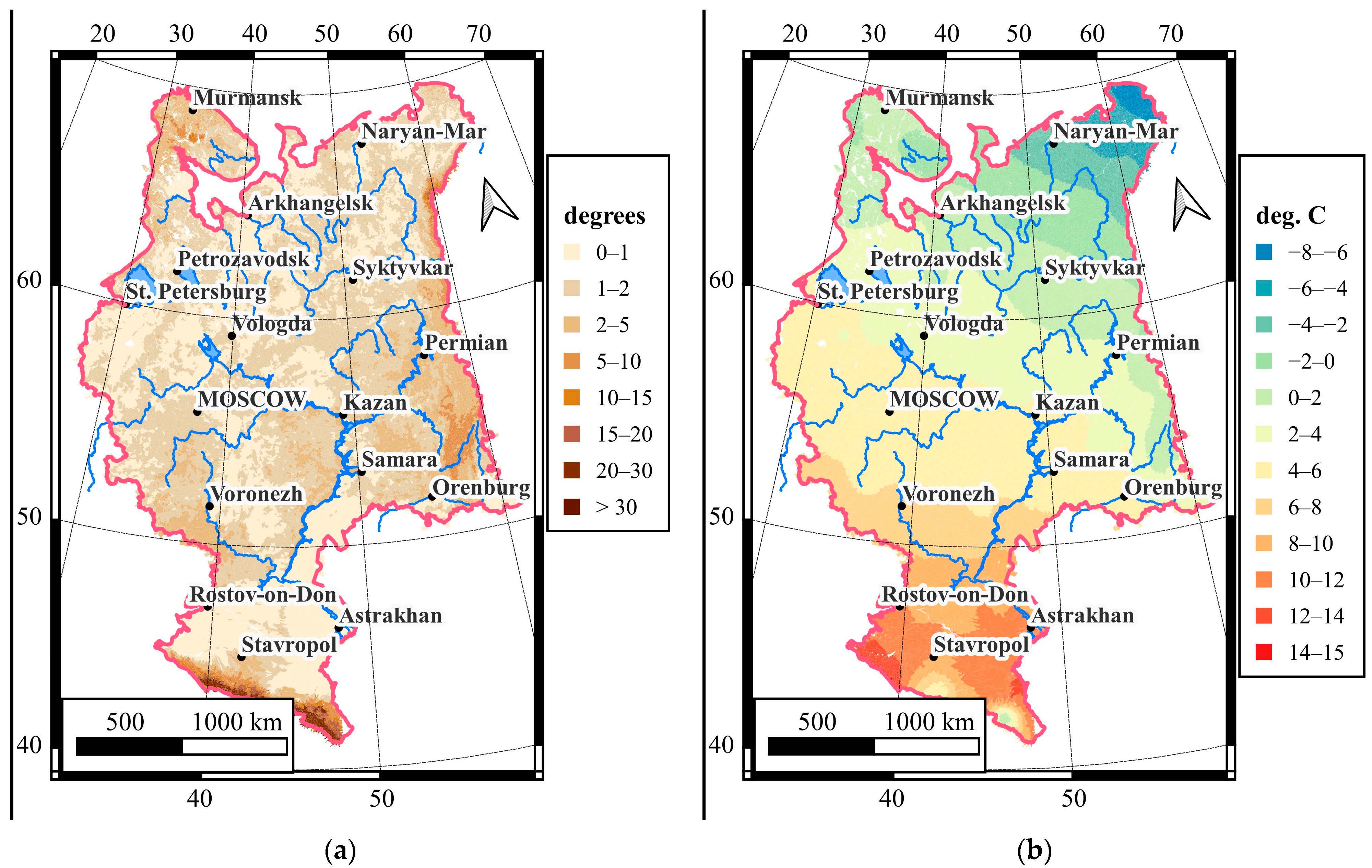
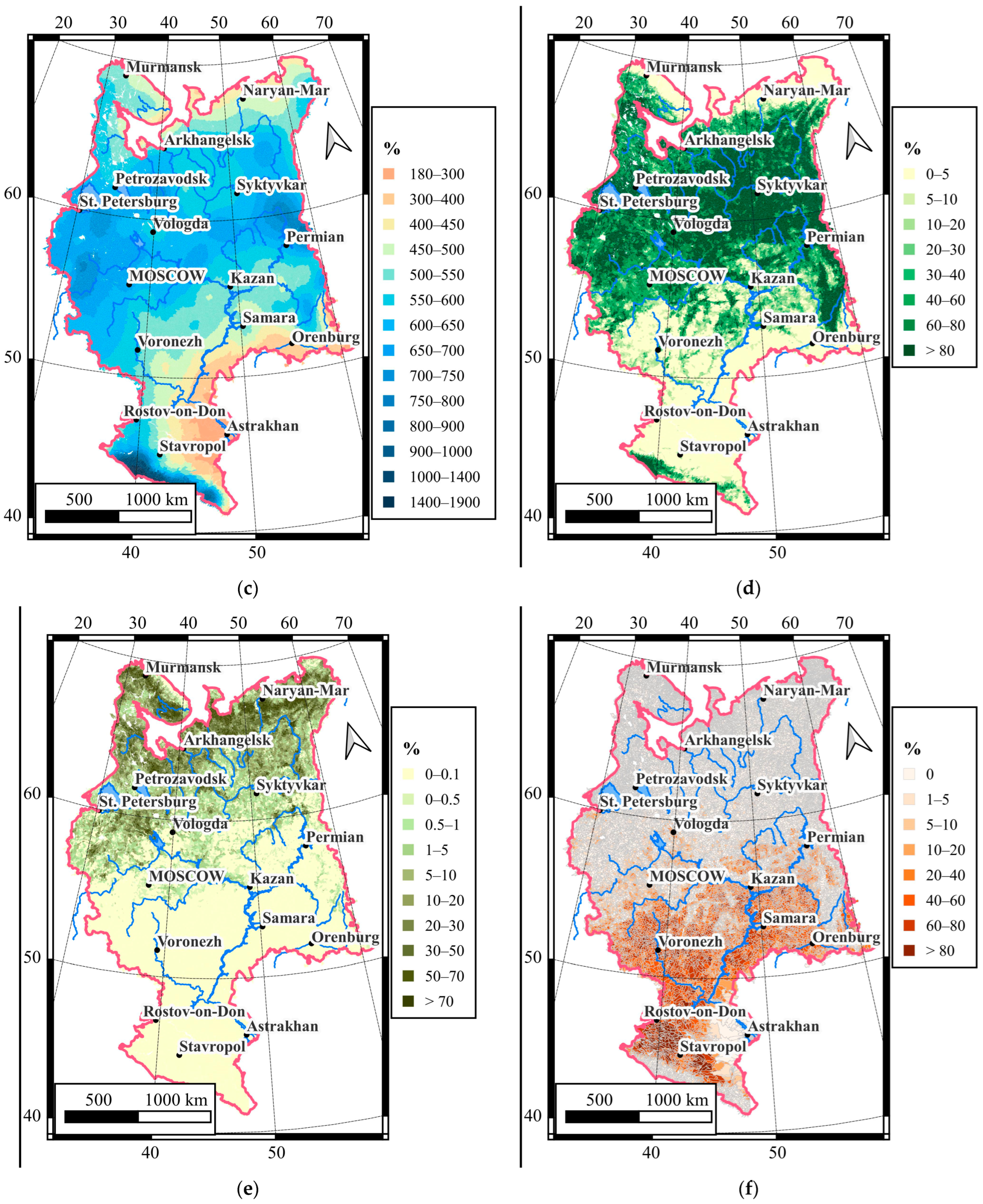
Figure 3.
Location of gauging stations provided with data on SSY in the plain regions of the EPR.

Figure 4.
Fragments of two basin grids: (a) the boundaries of the gauging station catchments; (b) the boundaries of the small river drainage basins.
Figure 4.
Fragments of two basin grids: (a) the boundaries of the gauging station catchments; (b) the boundaries of the small river drainage basins.

Figure 5.
Examples of the GAM model particular dependences of the logarithm of SSY per unit area on explanatory variables (horizontally—standardized predictor value, vertically—its contribution to model): (a) arable land percentage in basin where soil and soil-forming rock is strongly erodibility; (b) arable land percentage in basin where soil and soil-forming rock is moderately erodibility; (c) arable land percentage in basin where soil and soil-forming rock is resistant to eroding; (d) average steepness of slopes in basin.
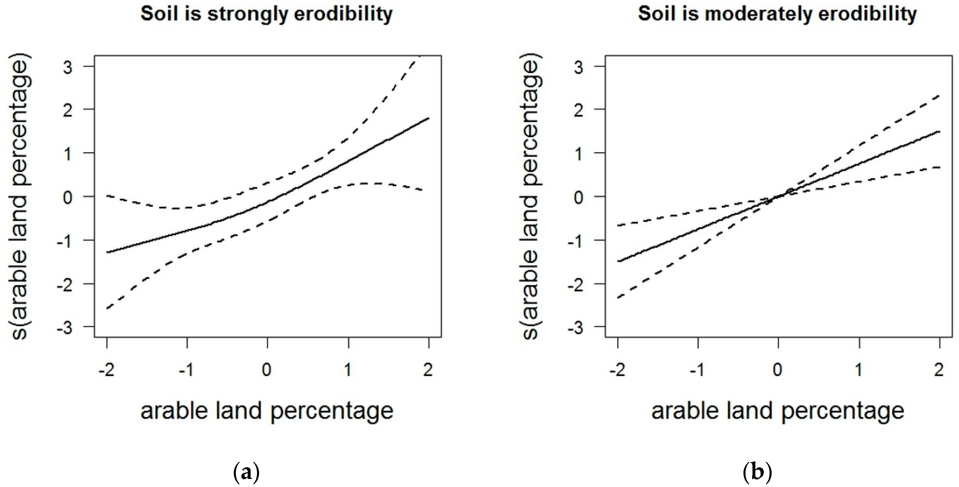
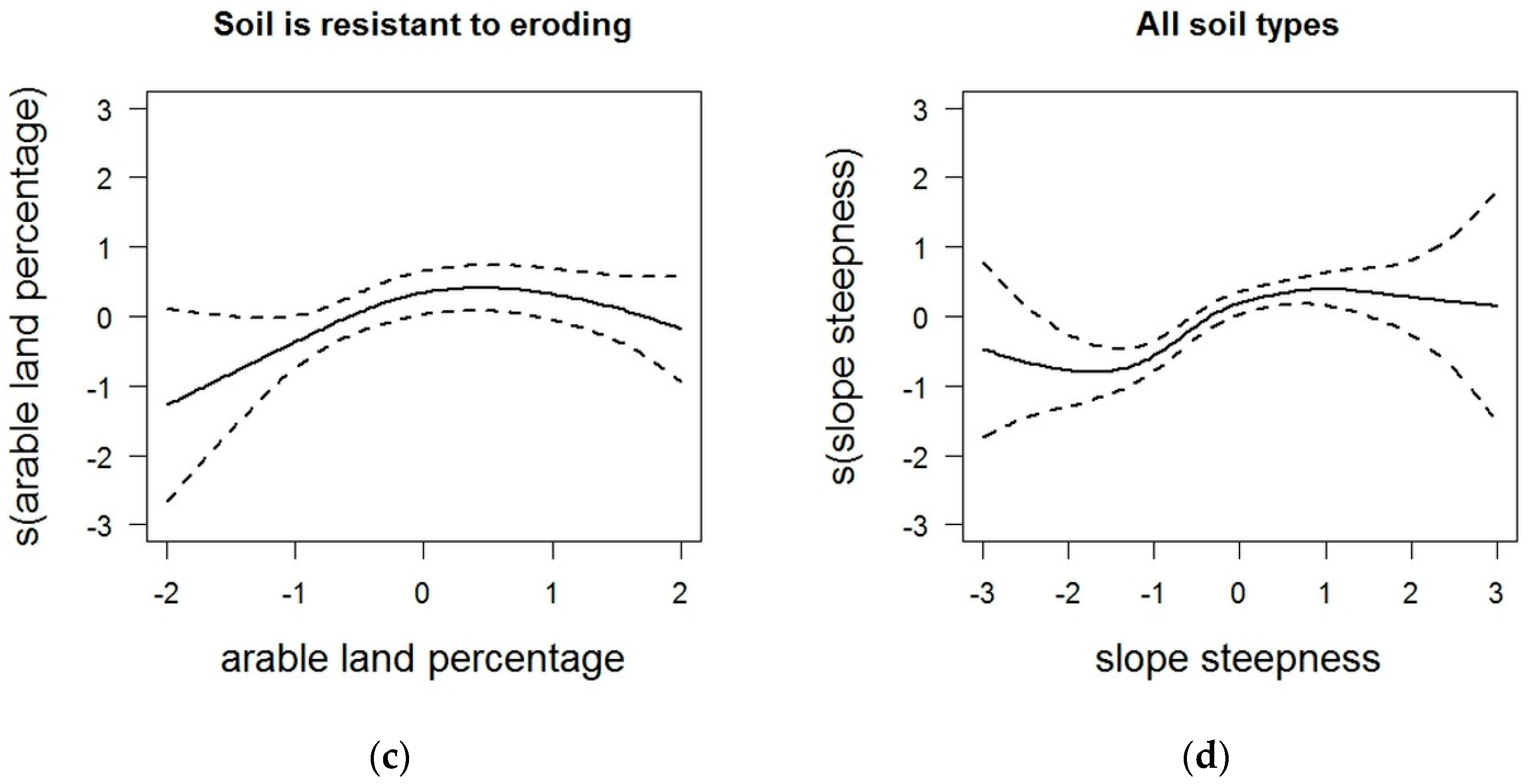
Figure 6.
Diagrams illustrating the quality of the constructed GLM model of the logarithm of SSY per unit: (a) observed values versus predicted values; (b) frequencies histogram of residuals values; (c) predicted values versus residuals; (d–f) model predictors values versus residuals.
Figure 6.
Diagrams illustrating the quality of the constructed GLM model of the logarithm of SSY per unit: (a) observed values versus predicted values; (b) frequencies histogram of residuals values; (c) predicted values versus residuals; (d–f) model predictors values versus residuals.

Figure 7.
Diagrams illustrating the quality of the constructed GAM model of the logarithm of SSY per unit: (a) observed values versus predicted values; (b) frequencies histogram of residuals values; (c) predicted values versus residuals; (d–f) model predictors values versus residuals.
Figure 7.
Diagrams illustrating the quality of the constructed GAM model of the logarithm of SSY per unit: (a) observed values versus predicted values; (b) frequencies histogram of residuals values; (c) predicted values versus residuals; (d–f) model predictors values versus residuals.

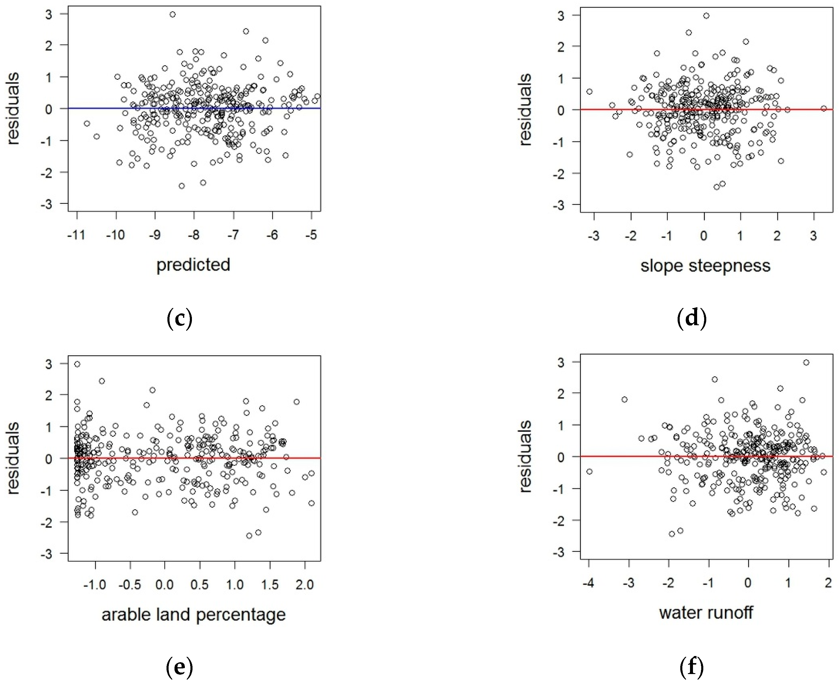
Figure 8.
Map of predicted values of the suspended sediment yield per unit (t per year per sq. km) for the river basins in the plains of the EPR. The prediction was obtained based on the GAM model.
Figure 8.
Map of predicted values of the suspended sediment yield per unit (t per year per sq. km) for the river basins in the plains of the EPR. The prediction was obtained based on the GAM model.


Table 1.
Landscape structure of the plain part of the EPR.
| Landscape Zone | Square, % |
|---|---|
| Tundra and forest-tundra | 8.8 |
| Northern taiga | 11.8 |
| Middle taiga | 16.2 |
| Southern taiga | 14.8 |
| Mixed and broad-leaved | 18.5 |
| Forest-steppe | 8.5 |
| Steppe | 16.9 |
| Semi-desert and desert | 4.6 |
Table 2.
Distribution of gauging stations by drainage basin area and duration of suspended sediment yield observations.
Table 2.
Distribution of gauging stations by drainage basin area and duration of suspended sediment yield observations.
| Basin Area, sq. km | Number of Observation Years | ||||||
|---|---|---|---|---|---|---|---|
| 1 to 10 | 10 to 20 | 20 to 30 | 30 to 40 | Over 40 | Total | % | |
| under 500 | 29 | 18 | 11 | 3 | 5 | 66 | 17.1 |
| 500–1000 | 14 | 15 | 12 | 5 | 2 | 48 | 12.5 |
| 1000–5000 | 64 | 50 | 22 | 11 | 14 | 161 | 41.8 |
| 5000–10,000 | 13 | 10 | 11 | 3 | 4 | 41 | 10.6 |
| 10,000–50,000 | 20 | 9 | 10 | 10 | 9 | 58 | 15.1 |
| 50,000–100,000 | 4 | 0 | 3 | 0 | 1 | 8 | 2.1 |
| over 100,000 | 1 | 1 | 0 | 0 | 1 | 3 | 0.8 |
| total | 145 | 103 | 69 | 32 | 36 | 385 | 100 |
| % | 37.7 | 26.8 | 17.9 | 8.3 | 9.4 | 100 | |
Table 3.
Sources of data about environmental conditions in basins of the study area.
| Explanatory Variables {X} | Data Source | Data Format |
|---|---|---|
| The terrain conditions | ||
| Average height Average steepness of slopes Average exposure Profile and plan curvatures Slope length Relief erosion potential | GMTED2010 with spatial resolution 250 m [36] | Raster data |
| Climatic characteristics | ||
| Annual precipitation Annual precipitation in May-August (heavy rain season) Precipitation for cold and warm periods of the year Variation coefficient of annual precipitation Annual average air temperature Average air temperature in January and in July Sum of active temperatures (sum of average daily temperatures for days when the temperature is above 10 °C) Average highs and lows of temperature Average amplitude of temperature Standard deviation of temperature Hydrothermic coefficient | Daily temperature and precipitation data on meteostations of Russia and USSR [38,39] | ASCII |
| The geological conditions | ||
| Class of pre-Quaternary deposits (predominant) | The “State geological map of the USSR of pre-Quaternary deposits” at a 1:1,000,000 scale | Vector data |
| The soil conditions | ||
| Type of soil (predominant) Type of soil-forming rock (predominant) | The Unified State Register of Soil Resources of Russia [40] | Vector data |
| Land cover/land use | ||
| Forest cover share Grassland cover share Brushwood cover share Swamp cover share Arable land share | TerraNorte RLC Map of the Russian Terrestrial Ecosystems, ver. 2015) (the Institute of Space Research of the Russian Academy of Sciences) [41] | Raster data |
| Landscape zones | ||
| Type of landscape (predominant) Subtype of landscape (predominant) | The “USSR Landscape Map” at a 1:2,500,000 scale | Vector data |
Table 4.
Significant variables and their coefficients for the GLM model of the logarithm of suspended sediment yield per unit area.
Table 4.
Significant variables and their coefficients for the GLM model of the logarithm of suspended sediment yield per unit area.
| Explanatory Variables | Transform | The Rank of Soil and Soil-Forming Rock Erodibility | Linear Model Coefficients |
|---|---|---|---|
| Average steepness of slopes | log | strongly erodibility | 0.176 |
| moderately erodibility | 0.684 | ||
| slightly erodibility | 0.592 | ||
| resistant to eroding | 0.333 | ||
| very resistant to eroding | 0.077 | ||
| Percentage of arable land | strongly erodibility | 1.673 | |
| moderately erodibility | 1.231 | ||
| slightly erodibility | 0.682 | ||
| resistant to eroding | 0.077 | ||
| very resistant to eroding | 0.198 | ||
| Water runoff per unit area | log | strongly erodibility | 1.246 |
| moderately erodibility | 0.718 | ||
| slightly erodibility | 0.405 | ||
| resistant to eroding | 0.503 | ||
| very resistant to eroding | 0.607 | ||
| Area of catchment | log | strongly erodibility | −0.038 |
| moderately erodibility | −0.083 | ||
| slightly erodibility | −0.237 | ||
| resistant to eroding | −0.192 | ||
| very resistant to eroding | −0.083 | ||
| Longitude | 0.408 | ||
| Latitude | −0.333 | ||
| Constant | −7.309 |
Table 5.
Residual statistics of the constructed logarithm models of the suspended sediment yield per unit.
Table 5.
Residual statistics of the constructed logarithm models of the suspended sediment yield per unit.
| Methods | ME | MdE | MAE | RMSE | WAPE | SE | R-Squared adj. |
|---|---|---|---|---|---|---|---|
| GLM | 8.8 | 0.0 | −0.005 | 0.746 | 1.031 | −0.096 | 0.993 |
| GAM | 11.8 | 0.0 | 0.064 | 0.592 | 0.845 | −0.076 | 0.781 |
Table 6.
Statistics of SSY per unit area for natural zones of study area.
| Landscape Zone | Min | 5% Quantile | Mean | Median | 95% Quantile | Max |
|---|---|---|---|---|---|---|
| Tundra and forest-tundra | 2.1 | 4.4 | 12.4 | 10.0 | 26.4 | 83.4 |
| Northern taiga | 2.1 | 3.8 | 12.1 | 10.8 | 24.4 | 91.1 |
| Middle taiga | 2.3 | 3.9 | 12.5 | 10.0 | 27.9 | 119.4 |
| Southern taiga | 1.8 | 2.5 | 11.8 | 6.4 | 34.0 | 116.1 |
| Mixed and broad-leaved | 0.8 | 2.9 | 25.1 | 13.9 | 90.0 | 226.5 |
| Forest-steppe | 0.6 | 5.2 | 33.5 | 28.0 | 87.2 | 158.4 |
| Steppe | 0.2 | 2.2 | 36.9 | 18.1 | 147.1 | 889.1 |
| Semi-desert and desert | 0.3 | 0.8 | 2.9 | 1.6 | 9.5 | 34.5 |
| Total | 0.24 | 46.2 | 17.3 | 10.9 | 46.2 | 1127.0 |
Disclaimer/Publisher’s Note: The statements, opinions and data contained in all publications are solely those of the individual author(s) and contributor(s) and not of MDPI and/or the editor(s). MDPI and/or the editor(s) disclaim responsibility for any injury to people or property resulting from any ideas, methods, instructions or products referred to in the content. |
© 2023 by the authors. Licensee MDPI, Basel, Switzerland. This article is an open access article distributed under the terms and conditions of the Creative Commons Attribution (CC BY) license (https://creativecommons.org/licenses/by/4.0/).
Share and Cite
MDPI and ACS Style
Yermolaev, O.; Mukharamova, S. Statistical Analysis and Modeling of Suspended Sediment Yield Dependence on Environmental Conditions. Water 2023, 15, 2639. https://doi.org/10.3390/w15142639
AMA Style
Yermolaev O, Mukharamova S. Statistical Analysis and Modeling of Suspended Sediment Yield Dependence on Environmental Conditions. Water. 2023; 15(14):2639. https://doi.org/10.3390/w15142639
Chicago/Turabian StyleYermolaev, Oleg, and Svetlana Mukharamova. 2023. "Statistical Analysis and Modeling of Suspended Sediment Yield Dependence on Environmental Conditions" Water 15, no. 14: 2639. https://doi.org/10.3390/w15142639
Note that from the first issue of 2016, this journal uses article numbers instead of page numbers. See further details here.