Inducing Evapotranspiration Reduction in an Engineered Natural System to Manage Saltcedar in Riparian Areas of Arid Environments

Abstract

Many management practices have been implemented to control non-native saltcedar (Tamarix spp.) in the Southwestern U.S. riparian areas. These management practices include herbicide application, mechanical and biological control. Despite these methods have had some success, they are not cost-efficient and some cases not easy to apply and can create environmental harm. In this study, we use a different approach where the mowing of saltcedar is timed according to the trend of evapotranspiration (ET) rates. The approach suppresses saltcedar growth, reduces ET loss, allows native vegetation to flourish, and eventually creates a healthy and diverse plant community in riparian areas. In an experimental study from 2010–2013, saltcedar was managed by mowing in a managed riparian area in New Mexico, USA. The timing of mowing was based on the observation of ET rates which were measured using the eddy covariance method. Normalized Difference Vegetation Index (NDVI) was calculated using Landsat imagery to observe any changes in vegetation of saltcedar before and after mowing and its correlation with ET. During the four years of measurement, it was observed that the timing of mowing led to a suppression of saltcedar, allowing the undergrowth of low water-consuming native grasses and other shrubs to thrive. Nonlinear mixed effects models of years of evapotranspiration during the season showed a significant reduction in ET in 2013 compared to the baseline year of 2010 across the growing stages, especially stage 2 (intercept of −2.0871 with p < 0.001). A reduction in ET of 32% from 1209 mm to 818 mm (difference of 391 mm) was observed between 2010 and 2013. This study showed that the best time to suppress saltcedar and allow native plants to reestablish, is to mow it before it breaks dormancy, at the peak and late parts of the growing season. Mowing can be discontinued once the native plants have been established.

1. Introduction

Saltcedar (Tamarix spp.) is an exotic deciduous shrub that grows best in riparian areas with shallow groundwater [1]. It is found mostly in floodplains and various alluvial soils influenced by adjacent rivers [2]. Saltcedar possesses many characteristics that allow it to outcompete native plants in riparian areas of arid environments in the Southwestern U.S. A saltcedar shrub can produce up to half a million small and light seeds per growing season. The seeds can disperse easily by wind and water, allowing them to spread along sandbars and riverbanks [3,4]. Saltcedar also spreads and reestablishes vegetatively in riparian areas and adjacent upland sites following flooding events [5]. Established saltcedars have deep root systems that allow them to access deeper groundwater in riparian areas than most native shallow-rooted plants. They can consume large amounts of water (i.e., evapotranspiration) ranging from 1000 mm to 1500 mm per year [6,7,8,9,10]. Saltcedar are facultative halophytes that can use saline groundwater by excreting excess salts through the leaf glands [5]. These saltcedar characteristics allow them to dominate native plants in riparian areas, creating a less diverse ecosystem.

Federal and state water management agencies and water irrigation districts have spent tremendous amounts of resources to manage saltcedar to improve the ecological health of riparian zones and establish indigenous plants such as willows, grasses, and other native species [11,12,13]. Management methods that have been used for controlling saltcedar include mechanical [14,15,16,17,18], chemical [19,20,21,22], and biological [23,24]. Estimated and actual costs of the different types of management practices have also been described by Hart et al. [11], Natale et al. [15], Shafroth et al. [16], Zavaleta [25], Taylor and McDaniel [26], and Barz et al. [27]. These management practices for controlling saltcedar vary in their effectiveness. Numerous studies have been conducted on the evapotranspiration (ET) of saltcedar [6,8,9,28]. The methods of measuring and estimating ET have also been documented in the literature [29,30,31]. The studies conducted by Culler et al. [6], Bawazir et al. [9], Hart et al. [11], and Weeks et al. [28] investigated the effects of saltcedar removal on ET by eradicating it. Managing saltcedar by eradication, however, has been less effective. The goal of this study is to manage saltcedar without complete eradication by timing the period of mowing based on ET observation. The benefits of this management method include reducing the density of saltcedar, improving plant diversity, reducing harm to the environment, and improving the chance of native low water consuming vegetation to reestablish while reducing ET depletion.

Furthermore, the normalized vegetation difference index (NDVI) was estimated using Landsat imagery to observe any changes in vegetation of saltcedar before and after mowing and its correlation with ET. The study’s findings may be used to: evaluate the current practices of managing saltcedar-dominated areas, improve the management of water and the riparian ET estimates in the hydrologic budget of a watershed, and make a decision on restoration efforts in riparian saltcedar dominated areas. It was hypothesized that continuously managing saltcedar by mowing would allow other low-water-consuming native plants to reestablish and ultimately reduce the density of saltcedar.

2. Materials and Methods

2.1. Experimental Site

The experiment was conducted on a 1000-hectare riparian land in the Rio Grande River flood plain between Elephant Butte and Caballo reservoirs in south-central New Mexico, USA (Figure 1). Sixty-four hectares within the 1000-hectare riparian land where a high percentage (>85%) of saltcedar bushes thrived was selected for the study. The vegetation in the plot consisted mainly of saltcedar mixed with sporadic vegetation. The sporadic vegetation at the site included: rayless goldenrod (Haplopappus heterophyllus (Torr. & A. Gray) Green), common cocklebur (Xanthium strumarium L.), seep willow (Baccharis salicifolia (Ruiz & Pav.) Pers.), honey mesquite (Prosopis juliflora (Sw.) DC), screw-bean mesquite (Prosopis pubescens Benth.), a few patches of saltgrass (Distichlis spectra (L.) Greene), bermuda grass (Cynodon dactylon (L.) Pers.), love grass (Eragrostis Watson), sedges (Cyperus esculentus L.), alkali sacaton (Sporobolus airoides (Torr.) Torr.), sixweeks grama (Bouteloua barbata Lag.), and sand dropseed (Sporobolus cryptandrus (Torr.) A. Gray).

The land at the site is generally flat (elevation 1283 m), with a mild slope towards the adjacent river east of the plot that provided an adequate fetch distance for an ET flux tower. The ET fetch measurements using the eddy covariance technique are further explained within this paper. The soils are typical of alluvial deposits with a texture of clay-silt-sandy loam, as determined from soil samples collected at the site. On the east and west of the floodplain are mountain ranges. Groundwater at the study site fluctuated with the river’s water stage but remained shallow within 3 m. The release of water from Elephant Butte controls the flow and stage of the river. Monsoon rains occasionally flooded the site from direct rainfall and the creeks that emptied into the river.

The Bureau of Reclamation (BoR), an agency that manages the reservoirs and dams in the southwestern United States, managed the spread and overgrowth of saltcedar at the riparian study area. In 1958 the BOR brush raked saltcedar to clear it. However, soon after, the saltcedar grew back and dominated the area. And since then, it has been mowed and treated with herbicide to control it [32].

The area’s climate is semiarid, with mean annual precipitation of 224 mm and ambient air temperature ranging from −20.5 °C in the winter to 41.1 °C in the summer [33]. The majority of precipitation occurs during the monsoon season from July to September. The topographic features surrounding the floodplain causes the prevailing winds at low elevations to blow mainly in the northerly-southerly directions.

2.2. Management of Saltcedar

Saltcedar was treated with herbicide in 2008 using a carpeted roller applicator, but the efficacy was low, and the plants grew back in 2009. It was then left to grow to maturity, becoming lush and dominating the area in 2010. The year 2010, when the saltcedar was mature and lush, was considered as the baseline for the study which extended from 2010 through 2013. Saltcedar was mowed on multiple occasions for the entire study area, once in 2011, and three times in 2013. Saltcedar was left to grow in 2012 to observe the effects of mowing from the previous year.

In 2011, saltcedar was mowed during the peak of the growing season in late July, the day of the year (DOY 208). The average height of salcedar after mowing in July 2011 was approximately 0.305 m (1 ft) and was left to grow during the rest of the year and growing season of 2012. The site was mowed again in 2013 on three separate occasions, during the dormancy period at the beginning of the year (DOY 18), in June (DOY 163) when saltcedar was lush and blooming, and after the peak of the growing season in September (DOY 252). Mowing saltcedar before the break of dormancy, and during the growing season is critical when plants are growing and transpiring. The effects of managing saltcedar by mowing during the study period was determined by comparing the measured ET rates and growing stages of vegetation.

2.3. Evapotranspiration Measurement

2.3.1. Energy Budget and Eddy Covariance Method

Evapotranspiration (ET) of saltcedar was determined by the energy budget and eddy covariance technique. Researchers have used the energy budget and eddy covariance methods to measure ET directly or determine ET as a residual of the energy budget of crops [34,35] and riparian vegetation [8,36]. As described by Allen et al. [37] and others (references therein), the eddy covariance technique is widely used around the world to measure sensible heat, latent heat, and gases such as carbon dioxide (CO₂) and methane (CH₄) fluxes. The factors governing the measurement accuracy of ET are described by Allen et al. [37]. A typical error, expressed as one standard deviation from the true mean value, for the eddy covariance method, can range from 15–30%, and the “Error for an experienced expert, trained and steeped in the physics of the process, %” can range from 10–15% [37]. Following Blanford and Gay [38], significant components of the energy budget (Rn, G, H) in the boundary layer were measured, and LE was determined as a residual (Equation (1)).

$$\mathrm{L}\mathrm{E}=\mathrm{R}\mathrm{n}-\mathrm{G}-\mathrm{H}$$

(1)

where LE is the latent heat flux in W/m² determined as a residual of the energy budget, Rn is the net radiation in W/m², G is the soil heat flux in W/m², and H is the sensible heat flux in W/m². The sign convention for the direction of the fluxes into and out of the boundary layer of the saltcedar area is such that Rn fluxes are positive when moving towards (adding energy) the hypothetical surface, and G, H, and LE are positive when moving away (removing energy) from the surface. The LE (W/m²) is divided by the latent heat of vaporization (λ in MJ/kg) and density of water (ρ in kg/m³) to obtain an equivalent depth of water or ET in mm. The latent heat of water varies slightly with temperature [29]. A constant value of 2.45 MJ/kg at a temperature of 20 °C was used because of the negligible difference (absolute error of <2%) over the typical ranges of temperatures observed (10–42 °C) in riparian areas of arid environments during the growing season. Similarly, the density of water of 1000 kg/m³ was used. The latent heat flux (LE) was calculated as a residual in the energy balance (Equation (1)) by measuring Rn, G, and H. In determining LE as a residual in the energy balance, a closure of 1.0 is assumed where energy consumed (LE + H) is equal to the available energy (Rn-G) and the biases in Rn, G, and H measurements transfer in LE estimate. The energy used in the photosynthesis process by plants or stored in the tree stems and canopy daily was considered negligible and therefore ignored in the energy budget. The H is measured using the eddy covariance technique [31,39], where vertical windspeed and air temperature in the lower boundary layer are correlated (Equation (2)).

$$\mathrm{H}=\overline{\mathsf{\rho }}{\mathrm{c}}_{\mathrm{p}}\left[\overline{{\mathrm{w}}^{\prime }{\mathrm{T}}^{\prime }}\right]$$

(2)

where, $\overline{\mathsf{\rho }}$ is the mean density of air (g/m³), c_p is the specific heat of air at constant pressure (J/g/°C), and $\overline{{\mathrm{w}}^{\prime }{\mathrm{T}}^{\prime }}$ is the covariance between fluctuations of vertical wind speed, w′, (m/s) and the temperature, T′, (°C). The overbar signifies the time average or sampling period of the product of instantaneous fluctuations.

2.3.2. Instrumentation

A triangulated tower was installed in the 64-ha plot (N 33°2′41.88″ and W 107°16′44.04″, 1283 m a.s.l.) and mounted with all the instrumentation. A pair of One Propeller Eddy Covariance (OPEC) systems were used to measure sensible heat at 8 Hz and averaged every 30 min [36,38,40]. The system consisted of two pairs of gill propeller anemometers (RM Young Company, Traverse City, MI, USA) and 75-μm fine wire thermocouples (Campbell Scientific Inc., Logan, UT, USA). The gill propeller anemometer measured vertical wind speed, and the thermocouple measured temperature. Two pairs of gill anemometers and fine wire thermocouples for the OPEC system were used to allow for consistency in data collection. The OPEC system was placed 6.3 m above the ground surface, providing adequate height above the canopy, considering the fetch distance. The eddy covariance technique requires adequate fetch distance or footprint to measure ET [41,42]. The fetch is an upwind distance contributing to the measurement site’s flux. The fetch distance from the flux tower to the edge of the study site in the horizontal distance stretched approximately 446 m to the south, 960 m to the Southwest, 240 m to the north, 146 m to the east, and 165 m to the west. During the experiment, most prevailing winds at the site occurred in the north-south direction. Air temperature and relative humidity were measured using an HMP45C temperature probe (Campbell Scientific, Inc., Logan, UT, USA) and placed 3.15 m above the ground surface. Windspeed and direction were measured using the 05103 wind monitor sensor (Campbell Scientific, Inc.) and placed at 3.71 m above the ground surface. Precipitation was measured using a tipping bucket rain gauge (Campbell Scientific, Inc.) and placed near the tower.

Net radiation was measured using a Q7.1 thermopile net radiometer (REBS, Inc., Seattle, WA, USA) placed 3.28 m above the ground surface. Net radiation data were collected at 1 Hz and averaged at 30-min intervals. Soil heat flux was measured using two HFT-3.1 soil heat flux plates (REBS Inc., Seattle, WA, USA), averaging soil temperature probes (TCAV), and CS616 water content reflectometer (Campbell Scientific Inc., Logan, UT, USA). Soil heat flux plates were placed about 1 m apart and 8 cm below the ground surface at locations underneath the saltcedar canopy and where saltcedar did not cover the ground. Averaging soil temperature probes were placed 2 cm and 6 cm below the ground surface in vertical alignment with soil heat flux plates. Soil volumetric moisture content was measured using a water content reflectometer. The reflectometer probe was inserted at a 45-degree angle in the top soil surface. All these measurements were collected at 8 Hz, averaged every 30 min, and stored on a CR23X datalogger (Campbell Scientific Inc., Logan, UT, USA). A battery charged by a solar panel powered the measurement system at the site.

The site was visited and maintained on a bi-weekly basis whenever possible. Data were filtered for those days when sensors were maintained (cleaned, replaced, etc.) or malfunctioned. Data considered as outliers were also filtered. A small number of ET data were fitted using an artificial neural network (ANN) following Abudu et al. [43] for infilling missing daily ET data. Maximum and minimum air temperature, maximum relative humidity, and solar radiation from a nearby weather station were used in the ANN to determine the daily missing ET values. The nearby weather station also measured precipitation, windspeed, and direction.

2.4. Groundwater

Depth to groundwater table (DWT) from the ground surface was measured using four WaterLOG^® pressure transducers with an enclosed datalogger (Design Analysis Associates, Inc., Logan, UT, USA) placed inside a 5.08 cm diameter polyvinyl chloride (PVC) pipe. The pipe was fully screened to about 30 cm below the ground surface with a slot size of 0.254 mm and a non-slotted casing 1-m pipe stick-up (above the ground). The manufacturer calibrated the pressure transducers and again checked in the hydraulics laboratory at New Mexico State University to ensure the depths measured were accurate. Data in the field were collected at a frequency of one minute and averaged every 30 min. Occasionally manual measurements were taken in the field using a water level sounder to check the pressure transducer values.

2.5. Vegetation Index

The Normalized Difference Vegetation Index (NDVI) was used to determine the growth and dynamics of managed saltcedar (i.e., before and after mowing) at the study site. NDVI has been used widely around the world by researchers as an indicator of vegetation growth and dynamics [44,45,46,47,48]. Plants use the energy in the red part of the spectrum for photosynthesis and reflect the near-infrared. The NDVI is calculated as a normalized ratio from the surface reflectance of wavelengths in the red (visible) and near-infrared spectral regions measured by satellite (Equation (3)).

$$\mathrm{N}\mathrm{D}\mathrm{V}\mathrm{I}=\frac{{(\mathsf{\rho }}_{\mathrm{N}\mathrm{I}\mathrm{R}}-{\mathsf{\rho }}_{\mathrm{R}\mathrm{e}\mathrm{d}})}{\left({\mathsf{\rho }}_{\mathrm{N}\mathrm{I}\mathrm{R}}+{\mathsf{\rho }}_{\mathrm{R}\mathrm{e}\mathrm{d}}\right)}$$

(3)

where ρ is the surface reflectance of wavelengths in the near-infrared (NIR) and red (Red) bands. Theoretically, the NDVI values vary between −1 and 1.

The NDVI was calculated from Landsat 5 Thematic Mapper (TM) bands 3-red (0.63–0.69 μm) and 4-near infrared (0.77–0.90 μm) and Landsat 8 Operational Land Imager (OLI) bands 4-red (0.64–0.67 μm) and 5-near infrared (0.85–0.88 μm) satellites. Satellite images were downloaded from the U.S. Geological Survey Earth Explorer website: https://earthexplorer.usgs.gov (accessed on 01 August 2019). Level 1 Terrain (L1T) images (i.e., data) with 30 m spatial resolution for each band, except for the 100 and 120 m resolution thermal infrared band by TM and OLI, respectively, were acquired for the study site’s clear sky days. Satellite data for 2010 and 2011 were obtained from Landsat 5 and 2013 from Landsat 8. No valuable data were available for 2012 from Landsat 7 due to scan line corrector (SLC) failure resulting in stripped data within the image. The L1T images are corrected for radiometric, geometric, and precision and use a digital elevation map (DEM) to correct parallax errors due to local topographic relief. Each satellite image was converted to radiance and then atmospherically corrected and converted to reflectance with FLAASH (Fast Line-of-sight Atmospheric Analysis of Spectral Hypercubes module) using ENVI (version 5.5) software^® (L3Harris Geospatial Co., Boulder, CO, USA) following methodology by Adler-Golden et al. [49]. An atmospheric model and K-T correction for aerosol scattering were selected within the FLAASH module [50]. Using the corrected values, the NDVI was calculated for all corrected images acquired in Landsat 5 TM and Landsat 8 OLI. From each image, 12 pixels (4 × 3 pixel matrices) were selected to represent the study site of managed saltcedar, which coincides with the area of measured ET. The calculated NDVI values from the 12 pixels were then averaged.

2.6. Statistical Analysis

Longitudinal associations of changes in ET over time among years using mixed-effects models were compared. Nonlinearity in time is handled by a cubic polynomial of the form $\mathrm{E}\mathrm{T}={\beta }_0+{\beta }_{1}t+{\beta }_2{t}^2$ + ${\beta }_3{t}^3$, where $t$ is the DOY for a particular growing stage in a given year and a first-order autoregressive structure [AR(1)] is assumed for the autocorrelation of errors. The nonlinear modeling with correlation structure was performed by R (version 4.2.0) using the Linear and Nonlinear Mixed Effects Models (nlme) package. In addition, NDVI was paired with ET to allow us to account for temporal trends. However, if the number of clear sky images (data) from the satellite needs to be larger to include time components in the association analysis between NDVI and ET, a separate comparison of correlations will be performed. Correlations for each stage of saltcedar growth during the season will be analyzed to describe the different stage effects on the associations.

3. Results

3.1. Evapotranspiration

Evapotranspiration was determined as a residual in the energy budget. Five-day moving average ET values and vapor pressure deficit (VPD) for the four years are shown in Figure 2. The annual ET was determined as 1209 mm (N = 365 days) in 2010, 1124 mm (N = 365 days) in 2011, 1040 mm (N = 366 days) in 2012, and 818 mm (N = 365 days) in 2013. The daily vapor pressure deficit (VPD) during the management period ranged from 0.09 kPa in the Fall to 4.24 kPa in the peak of the growing season (Figure 2). The VPD value is a good indicator of the demand for moisture in the air; the higher the VPD, the higher the demand for moisture. It is the difference between saturated and actual vapor pressure, calculated using air temperature and relative humidity following Allen et al. [51]. Mowing of saltcedar did not occur until mid-summer 2011 (Figure 3A,B). Saltcedar was mowed only once in 2011 (DOY 209) and was left to grow the following year to observe its effects after mowing once. In 2013, the site was mowed in January, June, and September (Figure 3C–F), allowing underbrush to thrive.

The fetch distance of eddy covariance measurements at the site, using the Lagrangian model following Kljun et al. [42,52], was determined to range from 37 to 841 m during the ET measurement period (i.e., 2010–2013). The average fetch distance during the four years was 262 m with a standard deviation of 76 m on a 30-min basis (N = 53,193 samples), falling within the boundaries of the study site.

During the middle of the growing season (i.e., DOY 208) before saltcedar was cut in 2011, the consumptive rate of water use by saltcedar was similar to that of the previous year, 2010. When saltcedar was mowed on July 28 (DOY 209) in 2011, the daily ET decreased from the previous day of 6.24 mm to 3.58 mm (41%) the day after. The ET remained low after mowing for about 23 days until monsoonal rains occurred. The following year 2012, saltcedar was left unmanaged and allowed to grow. However, the density of saltcedar at the site started to decrease, and undergrowth vegetation started to grow and flourish with more exposure to sunlight. In 2013, saltcedar was cut multiple times on DOY 18, 163, and 252. The first cut was early during the season and did not show a significant decline in ET since plants were still dormant. The saltcedar cuttings acted as a mulch to the soil reducing direct soil evaporation. During the second cut in June (DOY 163), ET decreased from 5.47 mm/day to 2.75 mm/day by DOY 165, a decrease of 50%. Mowing saltcedar in June further exposed more undergrowth vegetation to sunlight and allowed them to flourish. Evapotranspiration in June fluctuated and remained low for approximately 29 days (DOY 163–192). The sporadic saltcedar again grew vigorously after the second mowing in July due to several days of rainfall and plenty of soil moisture (Figure 3E). The third and final cut in September 2013 (DOY 252) during the rainy season was less effective. A decline in ET was observed only for two days after mowing but then increased due to regrowth and plenty of soil moisture from rainfall. Once the vegetation reached dormancy, the ET declined again. After a couple of years of treatment, the consumptive water use of saltcedar decreased over time (Figure 2).

Mixed effect models were conducted for changes in ET over time among years to detect the presence of autocorrelation. The cubic polynomial models showed an improvement over the linear mixed-effects model (all p < 0.005), resulting in a concave fitted curve with flat tails during winter. As shown in

Table 1. Nonlinear mixed effects models of years of evapotranspiration per growing stage. The * symbol indicates a significant difference in coefficient estimates of each polynomial component between years. The p-Value represents the significance of the overall temporal trend difference between years.

Years of Comparison	Growing Stages †	Day of Year (DOY)	Intercept (${\widehat{\mathit{\beta }}}_0$)	Linear (${\widehat{\mathit{\beta }}}_0$)	Quadratic (${\widehat{\mathit{\beta }}}_2$)	Cubic ${\widehat{\mathit{\beta }}}_2$	p-Value	Cumulative ET Difference (mm)
2011 vs. 2010	Stage 1	1–208	−0.0598	3.0110	−1.2975	−2.3871	0.0964	11.07
	Stage 2	209–270	−2.1011 *	6.8943 *	7.7590 *	−1.3448	<0.0001	129.32
	Stage 3	271–365	0.5841 *	1.3375	0.8782	−0.4750	0.6949	−55.63
							Total	84.76
2012 vs. 2011	Stage 1	1–208	−0.3221 *	−8.9818 *	0.8205	−2.4775	<0.0001	66.63
	Stage 2	209–270	1.0432 *	−7.6742 *	−4.0379 *	1.2676	0.0010	−64.01
	Stage 3	271–366	−0.8995 *	−0.0116	0.3088	−0.4920	0.9884	88.28
							Total	90.90
2013 vs. 2012	Stage 1	1–163	−0.8205 *	−0.6599	0.7909	5.4780 *	0.0002	134.02
	Stage 2	164–252	−0.9912 *	2.9892	0.6791	2.5485	0.4611	92.24
	Stage 3	253–366	0.0161	−1.0759	−1.5105	0.1738	0.7141	−3.65
							Total	222.61
2013 vs. 2010	Stage 1	1–163	−1.0394 *	−2.8818 *	4.2822 *	1.4705	<0.0001	169.70
	Stage 2	164–252	−2.0871 *	0.0703	−2.7958	−0.0405	0.6581	185.49
	Stage 3	253–365	−0.3602 *	2.0588	−1.9050	2.7277 *	0.0374	36.08
							Total	391.27

Notes: ^† Mowed once on DOY 209, 2011; Left to grow in 2012; mowed thrice on DOY 18, 163, & 252 in 2013.

, after the first mowing in 2011, a significant difference in trend can be observed for growing Stage 1. Curved trends in ET between the previous year and the following year were also significantly different for growing Stage 2 (i.e., after saltcedar was mowed), except for 2012–2013. In the second phase of 2013, a similar polynomial trend to that of 2012 was observed but found a significant decrease in the intercept term (p < 0.001). In Stage 3, after the growing season, the nonlinear pattern in ET did not differ across all-year comparisons. Significant reductions in ET were observed in 2013 compared to the baseline year of 2010 across the growing stages, especially for stage 2, with an estimated intercept of −2.0871 (p < 0.001).

3.2. Groundwater Measurements

Depths to groundwater table (DWT) from the ground surface of thirty-minute samples were collected from 2010 to 2013 using four pressure transducers with dataloggers from the monitoring wells (i.e., CA01, CA02, CA03, and CBT). Depths to groundwater table data were converted from 30-min means to daily means. Daily DWT, including precipitation from 2010 to 2013, is shown in Figure 4. Sensors for wells CA03 and CBT malfunctioned during the study due to clogging of the wells by fine soils. Long-term data was not collected. The DWT levels varied from 0.75 to 2.6 m. Fluctuation in DWT correlate with water released from the Elephant Butte Reservoir during the irrigation season and from several rainfall events. Due to prolonged drought in the region and less water being released from Elephant Butte Reservoir, an increase in DWT was observed over the years. On average, DWT from all piezometer wells was about 1.46 m in 2010, 1.60 m in 2011, 1.83 m in 2012, and 2.06 m in 2013 during the growing season. The DWT at the site is often deeper (~2.6 m) during the non-growing season when less water is released from Elephant Butte.

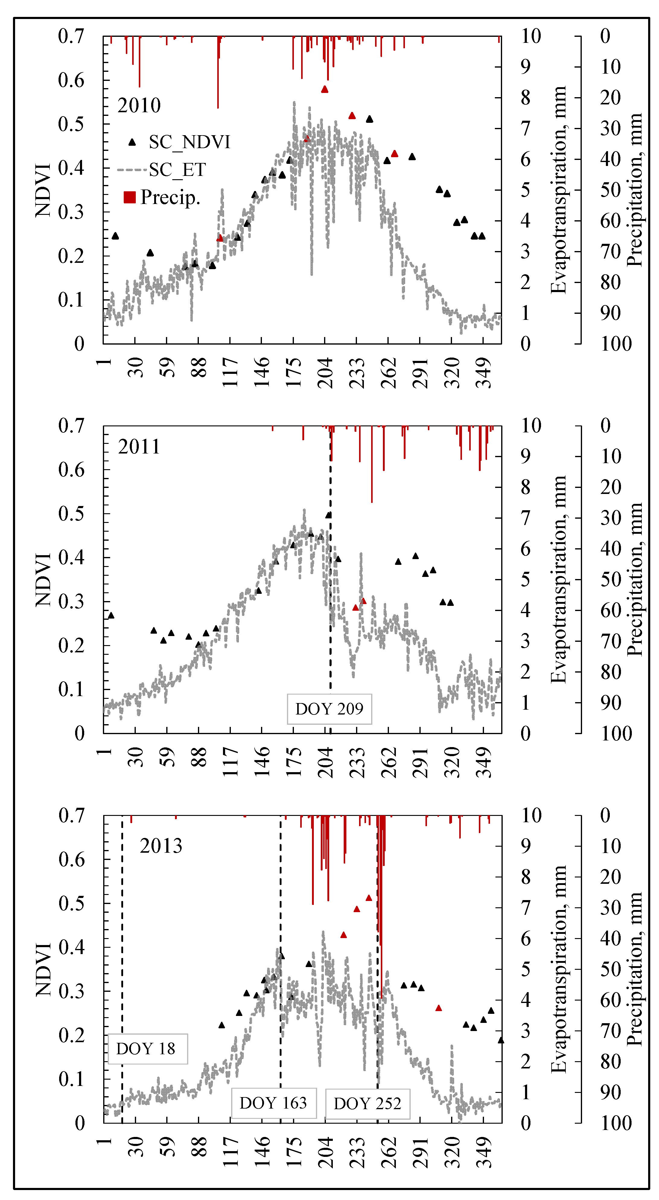
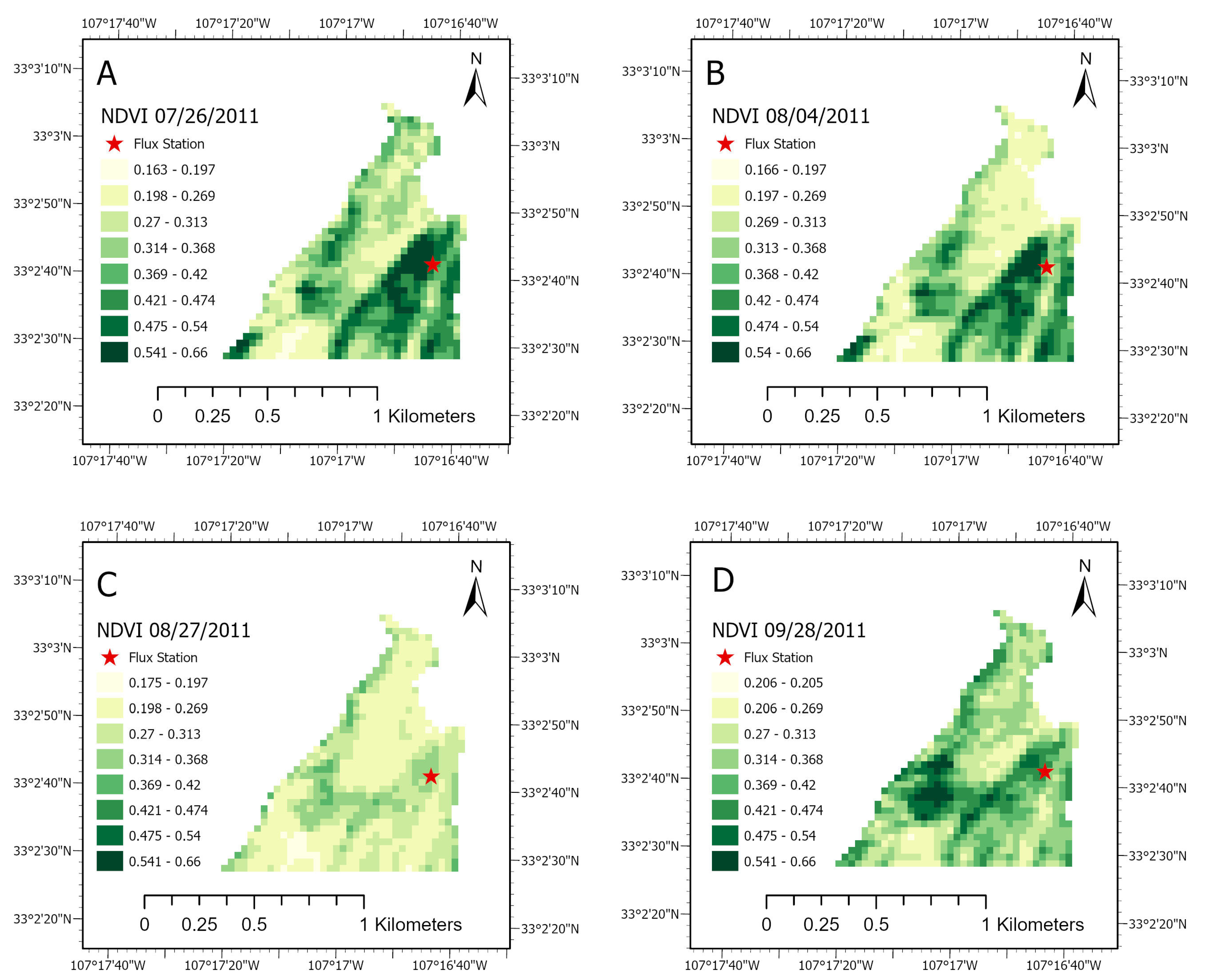
3.3. Normalized Vegetation Difference Index Measurements

Using satellite images from Landsat 5 TM and 8 OLI, NDVI was calculated for the managed saltcedar from 2010 to 2013, except for 2012. NDVI was not calculated during 2012 due to unavailable images from Landsat 5 TM satellite and stripped data drop-out images from Landsat 7 ETM+ satellite. Images from Landsat 8 were used for 2013; however, image collection did not begin until April since Landsat 8 was not launched until 11 February 2013. All the saltcedar leaves had fallen during the dormancy period, leaving saltcedar stems bare and exposing the ground surface to dormant underbrush vegetation and bare soil in some locations. This exposure allowed more light to reach the ground resulting in low NDVI values. The NDVI values began to increase after budbreak, reaching a peak and decreasing again due to senescence. The NDVI values of managed saltcedar followed similar trends as ET, where values peaked during the summer (DOYs 152 through 243) (Figure 5).

The growing season per annum at the managed saltcedar site averaged 241 days for four years (2010–2013). The leaves started budding at about DOY 71 and reached senescence by DOY 311. During 2010, NDVI reached 0.58 during the peak of the season. Some spikes in NDVI during that year are attributed to the moist soil from precipitation that occurred days prior (represented in red triangles in Figure 5). Darker pixilation shades of NDVI due to moist soil from precipitation during 2010–2013 are shown in Figure 6B,C, Figure 7B and Figure 8C,D. When mowing was conducted in 2011 and 2013, NDVI decreased following similar trends as ET (See Figure 5). These changes were also observed in Figure 7A–C and Figure 8A,B. When saltcedar grew again, NDVI began to increase until plants reached senescence. During the second cut of saltcedar in June 2013, NDVI dropped significantly. The second cut allowed the undergrowth of small vegetation and grasses to become dense and flourish. Although a significant drop in NDVI was shown due to the effect of mowing, values increased quickly after monsoonal rains. Plants accessed plenty of moisture in the soil, allowing them to become lusher with an increase in green foliage. However, after the soil moisture decreased, NDVI values declined until the plants were senesced. In combination with ET monitoring, readily available NDVI satellite images can be used to monitor and manage riparian vegetation’s health.

The NDVI sample size for each year was small due to the limited number of clear sky satellite data. Therefore, the time components in the association analysis between NDVI and ET were not performed. However, we performed a separate comparison of correlations for each stage to describe the different stage effects on the associations. Overall, the correlation between daily ET and NDVI during the growing season in 2010 (

Table 2. Comparisons of two correlation coefficients (ρ) between NDVI and ET and the corresponding p-values.

	2010 (N = 19) ρ = 0.6912, R2 = 48%	2011 (N = 17) ρ = 0.7858, R2 = 62%	2013 (N = 17) ρ = 0.5496, R2 = 30%
2010 (N = 19)	-
2011 (N = 17)	p-value = 0.5659	-
2013 (N = 17)	p-value = 0.5253	p-value = 0.2416	-

) was ρ = 0.6912 and R² = 0.4778 (N = 19). During 2011, the correlation increased (ρ = 0.7858, R² = 0.6175, N = 17) when saltcedar was cut once and then decreased during 2013 (ρ = 0.5496, R² = 0.3021, N = 17) when saltcedar was cut twice during the growing season. The correlation difference between 2011 and 2013 (

Table 3. Comparisons of two correlation coefficients (ρ) between NDVI and ET for 2011 and 2013 within the same growth stage.

	2011	2013	p-Value
Stage 1 (N = 10)	ρ = 0.9595, R2 = 92%	ρ = 0.6704, R2 = 45%	0.0084
Stage 2 (N = 3)	ρ = 0.9691, R2 = 94%	ρ = −0.3496, R2 = 12%	1.000
Stage 3 (N = 4)	ρ = 0.6668, R2 = 44%	ρ = 0.7226, R2 = 52%	0.9325

) was only significant for growing Stage 1 when the plants broke dormancy until they reached the peak of the season (ρ = 0.9595 for 2011, ρ = 0.6704 for 2013, and overall p-value = 0.0084). The lasting moisture in the ground after precipitation events and lack of sufficient clear sky Landsat images made it challenging to compare and provide a direct relation between NDVI and ET, especially when plants were mowed.

3.4. Climate

The maximum and minimum temperature, maximum and minimum relative humidity, and total precipitation measured from 2010 to 2013 are shown in

Table 4. Climatological data Measured at Caballo Mowed Saltcedar Study Site, Las Palomas, New Mexico. Maximum and Minimum Temperature (Temp._Max and Temp._ Min), Relative Humidity (RH_Max and RH_Min), and Total Precipitation (Precip.) N is the number of samples in days.

Year	Temp._Max °C	N	Temp._Min °C	N	RH_ Max %	N	RH_Min %	N	Precip. mm	N
2010	39.9	352	−11.4	352	97.0	352	5.2	352	184	352
2011	39.5	353	−21.0	353	97.4	353	3.6	353	181	353
2012	39.1	306	−11.3	306	96.3	306	2.8	306	84 *	306
2013	41.3	293	−14.1	293	94.5	293	3.1	293	153 *	293

Note: * some days of data collection were missing due to a malfunction of the rain gauge.

. The maximum and minimum temperature ranges are similar to that reported in Williams [33], where the maximum and minimum mean temperatures recorded from 1951–1980 for Truth or Consequences, NM, 8 km north of the study site, was 38.8 °C and −13.4 °C. High temperatures occurred during the summer months, while low temperatures occurred during the winter months, coinciding with literature gathered by Sheppard et al. [53]. The study site’s maximum and minimum relative humidity measurements ranged from less than 5% during dry months to about 98% in winter and after rainfall. During the July through September monsoon season, daily humidity values ranged from 23% to 88%.

Prevailing winds at the site were mostly in the north-south direction. During the growing season from April through July, the wind direction was mostly from the south and from August through October from the north. The 30-min average windspeeds during the growing season ranged from 1.8 m/s to 2.5 m/s, with gusts of 11.2 m/s to 13 m/s.

The total rainfall measured using a tipping bucket rain gauge during 2010, 2011, 2012, and 2013 was 184 mm (N = 352 days), 181 mm (N = 353 days), 84 mm (N = 306 days), and 153 mm (N = 293 days), respectively. A nearby climate station, also using a typing bucket rain gauge, measured for the same period (2010–2013) rainfall amounts of 208 mm (N = 365 days), 172 mm (N = 365 days), 97 mm (N = 366 days), and 374 mm (N = 365 mm). In 2013 the rain gauge at the study site malfunctioned and did not measure rainfall for the entire year. However, according to the measurements recorded at the nearby station, it was the wettest year. 2012 was the driest year, with less than 100 mm annual rainfall. Williams [33] reported a thirty-one-year (1951–1980) mean annual precipitation of 224 mm based on the data recorded at Truth or Consequences, NM. From 2010 to 2012, annual rainfall was below average, and in 2013 was above average. Most of the precipitation at the site occurred during July through September monsoonal season. The monsoonal season in New Mexico is defined by moisture coming from the Gulf of Mexico, leading to local high-intensity storms during the summer months of July through September [53]. The driest year was 2012, indicating severe drought conditions in the study area, which may be another reason saltcedar did not grow as vigorously.

4. Discussion

Non-native saltcedar in the riparian area of the Rio Grande at Palomas, New Mexico, was managed by mowing to allow native and non-native grasses and shrubs to thrive. The timing of mowing was based on ET observations at the site. The undergrowth of native and non-native grasses and shrubs over time was monitored using NDVI derived from satellite images. This study shows that NDVI can be useful for monitoring vegetation in riparian areas. However, interpreting NDVI requires some training skills to identify the vegetation status. Otherwise, other factors such as ponding water, moist soil after rainfall events, organic material on the ground, and plant senescence could skew the interpretation of NDVI values.

A reduction of ET and increased native vegetation growth were observed during the management period. Annual water consumption (or ET) of saltcedar decreased over time with increased mowing frequency and the timing of the mow and probably with declining water levels as shown by depths to groundwater over time. If saltcedar were left unmanaged and with available soil moisture, they would transpire to their potential and continue to flourish and dominate the site. Mowing was most effective for reducing ET and promoting the establishment of native vegetation when the plants are dormant in January, during the peak of the season in June, and after the monsoon season in September. Three mows per year can be repeated until the native vegetation dominates the area. At the beginning of the study in 2010, the annual ET of mature saltcedar was measured as 1209 mm. The ET measured was slightly less when compared to the values of a monotypic and dense stand of saltcedar reported in the literature. For example, Bawazir [54] measured an annual ET of 1325 mm using the eddy covariance method of a dense monotypic saltcedar on the Rio Grande floodplain. Using a lysimeter, Culler et al. [6] measured 1420 mm of annual ET of dense saltcedar on the Gila River floodplain. Blaney & Hanson [55] measured an annual ET of 1450 mm of dense saltcedar using a lysimeter at Carlsbad, New Mexico.

During the first mowing in 2011, a difference of 7% in ET (1209 mm vs. 1124 mm) was noted between 2010 and 2011. A reduction of 14% in ET (1209 mm vs. 1040 mm) between 2010 and 2012 was observed despite leaving saltcedar unmowed. The undergrowth vegetation started to emerge in 2012. A combination of undergrowth and a dry year with low precipitation (<100 mm/year) and soil moisture in the soil resulted in low ET in 2012. The following year, 2013, when saltcedar was cut three times, the reduction of ET between 2010 and 2013 was 32% (1209 vs. 818 mm). This reduction is comparable to Weeks et al. [28] findings, who reported a reduction of annual ET of about 30% when saltcedar was replaced by other vegetation (grass and forbs) in the Pecos River, New Mexico. Their study aimed to salvage groundwater by replacing saltcedar with other low-water-consuming vegetation. Culler et al. [6] investigated the ET reduction of saltcedar and mesquite before and after clearing it in the Gila River floodplain, Arizona. They estimated an average ET reduction of 44% or 480 mm. Slow changes in vegetation composition were observed at our study site during the first mowing but then progressed as the mowing continued over time. The reduction in ET during the study period is temporary until the saltgrass, small shrubs, and grasses are fully established. The dominating effect of replaced vegetation over saltcedar is illustrated in Figure 3.

Gonzalez et al. [13] reported the vegetation response to saltcedar control as part of a collaborative study of 416 sites. Methods of controlling saltcedar were divided into four categories: (1) hand-saw and chain-saw; (2) heavy machinery; (3) burning; and (4) biological control by defoliating beetle. They reported a reduction of up to 90% of saltcedar abundance due to burning and heavy machinery and approximately 50% due to biocontrol in dense saltcedar monoculture areas. They also reported increased native species over time through burning and saltcedar defoliation. In locations where sites were treated by cutting and heavy machinery, native grasses and grass-like plants doubled and almost tripled in cover. The increase in native cover correlated to permanent stream flow locations, less grazing pressure, more precipitation, low soil salinity, and low temperatures. Although the management of saltcedar proved beneficial for native species, Gonzalez et al. [13] study did not show enough significance overall, especially for native trees and shrubs. In locations where severe disturbances by either machinery or burning had occurred, secondary invasions of exotic forbs were experienced. According to Ostoja et al. [12], other consequences of removing saltcedar by heavy machinery resulted in removing or burying native plants and damaging the seeds. Leaving areas bare may lead to excessive temperatures, high soil evaporation, and increased soil salinity. Moreover, establishing native vegetation in these conditions by either pole planting, seeding, or germination by the natural establishment is challenging.

Due to mowing, adverse effects were not observed at the Caballo mowed saltcedar site. An increase of undergrowth vegetation, mainly saltgrass, and some extent of leaf litter from mowing in 2011 and follow-up treatment in 2013 allowed saltcedar to thin out during the study period. Other observed native species that were flourishing at the managed site in 2012 and 2013 included mesquite (Prosopis pubescens Benth.), seep-willow (Baccharis salicifolia (Ruiz & Pav.) Pers.), globe mallow (Sphaeralcea ambigua A. Gray), alkali sacaton (Sporobolus airoides (Torr.) Torr.) among others, indicating a decrease in saltcedar dominance. Most importantly, the timing of mowing contributed an essential role in managing saltcedar more effectively. Mowing saltcedar during the dormant period allowed the cuttings left on the ground to act as a mulch to the soil and reduced soil evaporation. In addition, it exposed the undergrowth plants to more sunlight. Mowing the second time when plants are actively growing allows the undergrowth plants, such as saltgrass and other native plants, to flourish and spread. The final cut allows saltcedar stands to thin out as native plants continue to spread after the monsoonal months. Mowing saltcedar three times a year is recommended to allow low water-consuming native plants to establish and dominate the area. There are several benefits to mowing: the saltcedar mulch and established grasses (e.g., saltgrass), including undergrowth vegetation, act as a barrier suppressing saltcedar seeds from germination and reducing water in the soil from evaporating [56,57].

Remote sensing imaging was used as a supplemental tool to monitor the effects of management by mowing and the changes in plant diversity. These effects are illustrated with NDVI (Figure 5, Figure 6, Figure 7 and Figure 8). The NDVI correlated well with the stages of mowing. The NDVI declined from a high value of 0.58 when saltcedar was dense to a low value of 0.30 when saltcedar was mowed. NDVI followed the same trend as the measured ET. Similarly, Snyder et al. [58] and Nagler et al. [59] observed a correlation between ET and NDVI during the biological control of saltcedar. Snyder et al. [58] measured ET and calculated NDVI before and after the defoliation of saltcedar by the Diorhabda carinulata (Tamarisk beetle). Before defoliation, NDVI during July through September ranged from 0.33 to 0.35. Once the beetles defoliated the saltcedar stands, NDVI ranged from 0.20 to 0.23. The ET followed the same trend as NDVI and decreased significantly from 5 mm/day to 1 mm/day. However, these NDVI and ET values are considerably lower than the Caballo mowed saltcedar study site. At the Caballo study site in 2010, before mowing, the NDVI during July through September ranged from 0.43 to 0.58. In 2011, when saltcedar was mowed once, the NDVI and ET decreased from 0.50 to 0.40 and ET from 6 mm/day to 4 mm/day. In 2013, the NDVI ranged from 0.29 to 0.38 when saltcedar was mowed three times, except for the days during the rainy season when NDVI ranged from 0.42 to 0.51. The ET fluctuated between 1.86 mm/day to 6.23 mm/day during the growing season with high values observed during the rainy season. The low-range ET reflects the effects of mowing and the dominance of low water-consuming saltgrass and brushes.

Overall, Snyder et al. [58] observed a correlation (R² = 0.48, p < 0.003) between the NDVI and 5-day average ET during the peak growing season periods of June through September. Their results were similar to those at the Caballo mowed saltcedar site. The correlation coefficient R² = 0.48, p < 0.001 was determined between ET and NDVI for 2010 when saltcedar was not mowed. However, the correlation between daily ET and NDVI during the growing season decreased significantly (R² = 0.62, p < 0.0002) from 2011 to 2013 (R² = 0.30, p < 0.022) due to the decoupling of ET from the green leaf area from multiple times of mowing in 2013. When comparing NDVI and ET during the growing Stage 1 (DOY 1–DOY 208) in 2011 and 2013, there was a correlation coefficient of 92% (R² = 0.9206, N = 10) and 45% (R² = 0.4494, N = 10), respectively. By the second stage, where mowing had occurred, the correlation increased to 94% (R² = 0.9392, N = 3) for 2011 but decreased for 2013 (R² = 12%, N = 3). Low correlation during mowing periods, especially in 2013, could be due to ponding water from previous rainfall events during Landsat acquisition. Additional clear sky images must be acquired to improve the correlation between the NDVI and ET. Clear sky days, however, are limited during the monsoonal season, where most days are cloudy.

Low values of NDVI and ET reported by Snyder et al. [58] could be attributed to the vegetation types at their study location. Although the site was dominated by saltcedar, the site also included areas of bare ground, remnants of cottonwood, coyote willow, and exotic Russian olive trees, with understory vegetation of rushes and perennial grasses. They reported that the mean understory canopy differed significantly during the measurement period. Canopy cover of native species during their initial measurement period decreased from 41% to 11%, whereas other vegetation covers, such as cheatgrass, expanded from 42% to 82%. Most of the underbrush at the Caballo mowed saltcedar study site was saltgrass and other small shrubs. After mowing, this led to more exposure of grasses to expand around the area.

5. Conclusions

This study illustrated that non-native saltcedar of the Southwestern US riparian areas could be managed effectively by timing the mowing based on the upward trend of ET observations. The timing of mowing was an important factor in the management of saltcedar to reduce its dominance. The best time for mowing in the Southwestern U.S. is in late January and then again in June before the rainfall season, and late September after the rainfall season. In other locations, the best time for mowing would be before the saltcedar breaks dormancy to allow undergrowth vegetation an early chance to grow, and at the peak and late parts of the growing season. As a result of managing saltcedar to allow grasses and shrubs to grow, total ET was reduced by 32% or 391 mm (1209 mm to 818 mm) from 2010 to 2013. It is cost-effective in the long term management of saltcedar if it is mowed for consecutive years. The spread of saltgrass, other types of grasses, and brushes increased at the site as the density and germination of saltcedar declined. The limitation of this study is that it was not replicated and the experiment was conducted at only one location. It is suggested that further studies be conducted at other locations to verify the management technique. The NDVI derived from remote sensing correlated with ET reduction during the four years of monitoring. For management purposes, NDVI can be essential for tracking changes in the saltcedar density over time in riparian areas.

References

1. McDaniel, K.C.; DiTomaso, J.M.; Duncan, C.A. Tamarisk or saltcedar, Tamarix spp. In Assessing the Economic, Environmental and Societal Losses from Invasive Plants on Rangeland and Wildlands; Clark, J.K., Duncan, C.L., Eds.; Weed Science Society of America: Champaign, IL, USA, 2005; pp. 198–222. [Google Scholar]
2. Taylor, J.P.; McDaniel, K.C. Restoration of Saltcedar (Tamarix Spp.)-Infested Floodplains on the Bosque Del Apache National Wildlife Refuge. Weed Technol. 1998, 12, 345–352. [Google Scholar] [CrossRef]
3. Brotherson, J.D.; Field, D. Tamarix: Impacts of a Successful Weed. Rangelands 1987, 9, 110–112. [Google Scholar]
4. Di Tomaso, J.M. Impact, Biology, and Ecology of Saltcedar (Tamarix Spp.) in the Southwestern United States. Weed Technol. 1998, 12, 326–336. [Google Scholar] [CrossRef]
5. Carruthers, R.I.; Deloach, C.J.; Herr, J.C.; Anderson, G.L.; Knutson, A.E. Salt Cedar Areawide Pest Management in the Western USA. In Areawide Pest Management: Theory and Implementation; Koul, O., Cuperus, G.W., Elliott, N., Eds.; CABI: Wallingford, UK, 2008; pp. 271–299. [Google Scholar]
6. Culler, R.C.; Hanson, R.L.; Myrick, R.M.; Turner, R.; Kipple, F. Evapotranspiration before and after Clearing Phreatophytes, Gila River Flood Plain, Graham County, Arizona; United States Geological Survey: Reston, VA, USA, 1982. [Google Scholar]
7. Devitt, D.A.; Sala, A.; Smith, S.D.; Cleverly, J.; Shaulis, L.K.; Hammett, R. Bowen Ratio Estimates of Evapotranspiration for Tamarix ramosissima Stands on the Virgin River in Southern Nevada. Water Resour. Res. 1998, 34, 2407–2414. [Google Scholar] [CrossRef]
8. Cleverly, J.R.; Dahm, C.N.; Thibault, J.R.; Gilroy, D.J.; Allred Coonrod, J.E. Seasonal Estimates of Actual Evapo-Transpiration from Tamarix Ramosissima Stands Using Three-Dimensional Eddy Covariance. J. Arid Environ. 2002, 52, 181–197. [Google Scholar] [CrossRef]
9. Bawazir, A.S.; King, J.P.; Kidambi, S.; Tanzy, B.; Stowe, N.H.; Fahl, M.J. A Joint Investigation of Evapotranspiration Depletion of Treated and Non-Treated Saltcedar at the Elephant Butte Delta, New Mexico; New Mexico Water Resources Research Institute: Las Cruces, NM, USA, 2006. [Google Scholar]
10. Westenburg, C.L.; Harper, D.P.; DeMeo, G.A. Evapotranspiration by Phreatophytes along the Lower Colorado River at Havasu National Wildlife Refuge, Arizona; United States Geological Survey: Reston, VA, USA, 2006. [Google Scholar]
11. Hart, C.R.; White, L.D.; McDonald, A.; Sheng, Z. Saltcedar Control and Water Salvage on the Pecos River, Texas, 1999–2003. J. Environ. Manag. 2005, 75, 399–409. [Google Scholar] [CrossRef]
12. Ostoja, S.M.; Brooks, M.L.; Dudley, T.; Lee, S.R. Short-Term Vegetation Response Following Mechanical Control of Saltcedar (Tamarix Spp.) on the Virgin River, Nevada, USA. Invasive Plant Sci. Manag. 2014, 7, 310–319. [Google Scholar] [CrossRef]
13. González, E.; Sher, A.A.; Anderson, R.M.; Bay, R.F.; Bean, D.W.; Bissonnete, G.J.; Bourgeois, B.; Cooper, D.J.; Dohrenwend, K.; Eichhorst, K.D.; et al. Vegetation Response to Invasive Tamarix Control in Southwestern U.S. Rivers: A Collaborative Study Including 416 Sites. Ecol. Appl. 2017, 27, 1789–1804. [Google Scholar] [CrossRef]
14. Taylor, J.P.; McDaniel, K.C. Riparian Management On The Bosque Del Apache National Wildlife Refugee. N. M. J. Sci. 1998, 38, 219–232. [Google Scholar]
15. Natale, E.; Sorli, L.; De La Reta, M.; Coria, G.; Zilio, M.; Arana, M.D.; Aros, L.; Estive, F.; Palma, M.; Oggero, A.J. Basis for Restoration of Saltcedar (Tamarix Spp., Tamaricaceae) Invaded Sites through an Adaptive Management Approach. J. Nat. Conserv. 2022, 68, 126230. [Google Scholar] [CrossRef]
16. Shafroth, P.B.; Brown, C.A.; Merritt, D.M. Saltcedar and Russian Olive Control Demonstration Act Science Assessment; United States Geological Survey: Reston, VA, USA, 2010. [Google Scholar]
17. McDaniel, K.C.; Taylor, J.P. Saltcedar Recovery after Herbicide-Burn and Mechanical Clearing Practices. J. Range Manag. 2003, 56, 439–445. [Google Scholar] [CrossRef]
18. Fick, W.H.; Geyer, W.A. Cut-Stump Treatment of Saltcedar (Tamarix ramosissima) on the Cimarron National Grasslands. Trans. Kans. Acad. Sci. 2010, 113, 223–226. [Google Scholar] [CrossRef]
19. Duncan, K.W.; McDaniel, K.C. Saltcedar (Tamarix Spp.) Management with Imazapyr. Weed Technol. 1998, 12, 337–344. [Google Scholar] [CrossRef]
20. McDaniel, K.C.; Taylor, J.P. Aerial Spraying and Mechanical Saltcedar Control. In Saltcedar and Water Resources in the West Symposium; The Texas Agricultural Experiment Station: San Angelo, TX, USA, 2003; pp. 100–105. [Google Scholar]
21. Duncan, K.W. Individual Plant Treatment of Saltcedar. In Saltcedar and Water Resources in the West Symposium; Texas Agricultural Experiment Station: San Angelo, TX, USA, 2003; pp. 106–110. [Google Scholar]
22. Douglass, C.H.; Nissen, S.J.; Kniss, A.R. Efficacy and Environmental Fate of Imazapyr from Directed Helicopter Applications Targeting Tamarix Species Infestations in Colorado: Helicopter Imazapyr Applications to Control Tamarix spp. Pest. Manag. Sci. 2016, 72, 379–387. [Google Scholar] [CrossRef] [PubMed]
23. DeLoach, C.J.; Carruthers, R.I.; Dudley, T.L.; Eberts, D.; Kazmer, D.J.; Knutson, A.E.; Bean, D.W.; Knight, J.; Lewis, P.A.; Milbrath, L.R.; et al. First Results for Control of Saltcedar (Tamarix spp.) in the Open Field in the Western United States. In XI International Symposium on Biological Control of Weeds; CSIRO Entomology: Canberra, Australia, 2004; pp. 505–513. [Google Scholar]
24. Hudgeons, J.L.; Knutson, A.E.; Heinz, K.M.; DeLoach, C.J.; Dudley, T.L.; Pattison, R.R.; Kiniry, J.R. Defoliation by Introduced Diorhabda Elongata Leaf Beetles (Coleoptera: Chrysomelidae) Reduces Carbohydrate Reserves and Regrowth of Tamarix (Tamaricaceae). Biol. Control 2007, 43, 213–221. [Google Scholar] [CrossRef]
25. Zavaleta, E. Valuing Ecosystem Services Lost to Tamarix Invasion in the United States. In Invasive Species in A Changing World; Mooney, H.A., Hobbs, R.J., Eds.; Island Press: Washington DC, USA, 2000; pp. 261–300. [Google Scholar]
26. Taylor, J.P.; McDaniel, K.C. Revegetation Strategies After Saltcedar (Tamarix spp.) Control in Headwater, Transitional, and Depositional Watershed Areas. Weed Technol. 2004, 18, 1278–1282. [Google Scholar]
27. Barz, D.; Watson, R.P.; Kanney, J.F.; Roberts, J.D.; Groeneveld, D.P. Cost/Benefit Considerations for Recent Saltcedar Control, Middle Pecos River, New Mexico. Environ. Manag. 2009, 43, 282–298. [Google Scholar] [CrossRef]
28. Weeks, E.P.; Weaver, H.L.; Campbell, G.S.; Tanner, B.D. Water Use by Saltcedar and by Replacement Vegetation in the Pecos River; United States Geological Survey: Reston, VA, USA, 1987. [Google Scholar]
29. Jensen, M.E.; Burman, R.D.; Allen, R.G. Evapotranspiration and Irrigation Water Requirements: A Manual; American Society of Civil Engineers, Ed.; ASCE manuals and reports on engineering practice; The Society: New York, NY, USA, 1990; ISBN 9780872627635. [Google Scholar]
30. Dingman, S.L. Physical Hydrology; Prentice-Hall, Inc.: Upper Saddle, NJ, USA, 2002. [Google Scholar]
31. Brutsaert, W. Hydrology: An Introduction; Cambridge University Press: Cambridge, UK, 2005. [Google Scholar]
32. Tanzy, B.F. (United States Bureau of Reclamation, Elephant Butte, NM, USA). Personal Communication. 2008. [Google Scholar]
33. Williams, J.L. New Mexico in Maps, 2nd ed.; Universtiy of New Mexico Press: Albuquerque, NM, USA, 1986. [Google Scholar]
34. Samani, Z.; Bawazir, A.S.; Bleiweiss, M.; Skaggs, R.; Longworth, J.; Tran, V.D.; Pinon-Villarreal, A. Using Remote Sensing to Evaluate the Spatial Variability of Evapotranspiration and Crop Coefficient in the Lower Rio Grande Valley, New Mexico. Irrig. Sci. 2009, 28, 93–100. [Google Scholar] [CrossRef]
35. Eshonkulov, R.; Poyda, A.; Ingwersen, J.; Wizemann, H.D.; Weber, T.K.; Kremer, P.; Hogy, P.; Pulatov, A.; Streck, T. Evaluating Multi-Year, Multi-Site Data on the Energy Balance Closure of Eddy-Covariance Flux Measurements at Cropland Sites in Southwestern Germany. Biogeosciences 2019, 16, 521–540. [Google Scholar] [CrossRef]
36. Bawazir, A.S.; Samani, Z.; Bleiweiss, M.; Skaggs, R.; Schmugge, T. Using ASTER Satellite Data to Calculate Riparian Evapotranspiration in the Middle Rio Grande, New Mexico. Int. J. Remote Sens. 2009, 30, 5593–5603. [Google Scholar] [CrossRef]
37. Allen, R.G.; Pereira, L.S.; Howell, T.A.; Jensen, M.E. Evapotranspiration Information Reporting: I. Factors Governing Measurement Accuracy. Agric. Water Manag. 2011, 98, 899–920. [Google Scholar] [CrossRef]
38. Blanford, J.H.; Gay, L.W. Tests of a Robust Eddy Correlation System for Sensible Heat Flux. Theor. Appl. Clim. 1992, 46, 53–60. [Google Scholar] [CrossRef]
39. Swinbank, W.C. The Measurement of Vertical Transfer of Heat and Water Vapor by Eddies in the Lower Atmosphere. J. Meteor. 1951, 8, 135–145. [Google Scholar] [CrossRef]
40. Amiro, B.D.; Wuschke, E.E. Evapotranspiration from a Boreal Forest Drainage Basin Using an Energy Balance/Eddy Correlation Technique. Bound.-Layer Meteorol. 1987, 38, 125–139. [Google Scholar] [CrossRef]
41. Schmid, H.P. Footprint Modeling for Vegetation Atmosphere Exchange Studies: A Review and Perspective. Agric. For. Meteorol. 2002, 113, 159–183. [Google Scholar] [CrossRef]
42. Kljun, N.; Calanca, P.; Rotach, M.W.; Schmid, H.P. A Simple Parameterisation for Flux Footprint Predictions. Bound.-Layer Meteorol. 2004, 112, 503–523. [Google Scholar] [CrossRef]
43. Abudu, S.; Bawazir, A.S.; King, J.P. Infilling Missing Daily Evapotranspiration Data Using Neural Networks. J. Irrig. Drain Eng. 2010, 136, 317–325. [Google Scholar] [CrossRef]
44. Tucker, C.J.; Fung, I.Y.; Keeling, C.D.; Gammon, R.H. Relationship between Atmospheric CO2 Variations and a Satellite-Derived Vegetation Index. Nature 1986, 319, 195–199. [Google Scholar] [CrossRef]
45. Lenney, M.P.; Woodcock, C.E.; Collins, J.B.; Hamdi, H. The Status of Agricultural Lands in Egypt: The Use of Multitemporal NDVI Features Derived from Landsat TM. Remote Sens. Environ. 1996, 56, 8–20. [Google Scholar] [CrossRef]
46. Nemani, R.R.; Keeling, C.D.; Hashimoto, H.; Jolly, W.M.; Piper, S.C.; Tucker, C.J.; Myneni, R.B.; Running, S.W. Climate-Driven Increases in Global Terrestrial Net Primary Production from 1982 to 1999. Science 2003, 300, 1560–1563. [Google Scholar] [CrossRef]
47. Donohue, R.J.; McVICAR, T.R.; Roderick, M.L. Climate-related Trends in Australian Vegetation Cover as Inferred from Satellite Observations, 1981–2006. Glob. Change Biol. 2009, 15, 1025–1039. [Google Scholar] [CrossRef]
48. Gandhi, G.M.; Parthiban, S.; Thummalu, N.; Christy, A. Ndvi: Vegetation Change Detection Using Remote Sensing and Gis—A Case Study of Vellore District. Procedia Comput. Sci. 2015, 57, 1199–1210. [Google Scholar] [CrossRef]
49. Adler-Golden, S.M.; Matthew, M.W.; Bernstein, L.S.; Levine, R.Y.; Berk, A.; Richtsmeier, S.C.; Acharya, P.K.; Anderson, G.P.; Felde, J.W.; Gardner, J.A.; et al. Atmospheric Correction for Shortwave Spectral Imagery Based on MODTRAN4; Descour, M.R., Shen, S.S., Eds.; SPIE: Denver, CO, USA, 1999; pp. 61–69. [Google Scholar]
50. Kaufman, Y.J.; Tanré, D.; Gordon, H.R.; Nakajima, T.; Lenoble, J.; Frouin, R.; Grassl, H.; Herman, B.M.; King, M.D.; Teillet, P.M. Passive Remote Sensing of Tropospheric Aerosol and Atmospheric Correction for the Aerosol Effect. J. Geophys. Res. 1997, 102, 16815–16830. [Google Scholar] [CrossRef]
51. Kljun, N.; Rotach, M.W.; Schmid, H.P. A Three-Dimensional Backward Lagrangian Footprint Model For A Wide Range Of Boundary-Layer Stratifications. Bound.-Layer Meteorol. 2002, 103, 205–226. [Google Scholar] [CrossRef]
52. Allen, R.G. The ASCE Standardized Reference Evapotranspiration Equation; Environmental and Water Resources institute (U.S.), Ed.; American Society of Civil Engineers: Reston, VA, USA, 2005; ISBN 9780784408056. [Google Scholar]
53. Sheppard, P.; Comrie, A.; Packin, G.; Angersbach, K.; Hughes, M. The Climate of the US Southwest. Clim. Res. 2002, 21, 219–238. [Google Scholar] [CrossRef]
54. Bawazir, A.S. Saltcedar and Cottonwood Riparian Evapotranspiration in the Middle Rio Grande. Ph.D. Dissertation, New Mexico State University, Las Cruces, NM, USA, 2000. [Google Scholar]
55. Blaney, H.F.; Hanson, E.G. Consumptive Use and Water Requirements in New Mexico; New Mexico State Engineer Office; Santa Fe, NM, USA, 1965; pp. 1–82 & 3 folded maps.
56. Lair, K.D. Revegetation Strategies and Technologies for Restoration of Aridic Saltcedar (Tamarix spp.) Infestation Sites. In Proceedings of the National Proceedings: Forest and Conservation Nursery Associations—2005, Fort Collins, CO, USA, 26–28 July 2005; U.S. Department of Agriculture Forest Service: Washington, DC, USA, 2006; pp. 10–20. [Google Scholar]
57. Grundy, A.C.; Bond, B. Use of Non-Living Mulches for Weed Control. In Non-Chemical Weed Management: Principles, Concepts and Technology; Blackshaw, R.E., Upadhyaya, M.K., Eds.; CABI: Wallingford, UK, 2007. [Google Scholar]
58. Snyder, K.A.; Scott, R.L.; McGwire, K. Multiple Year Effects of a Biological Control Agent (Diorhabda carinulata) on Tamarix (Saltcedar) Ecosystem Exchanges of Carbon Dioxide and Water. Agric. For. Meteorol. 2012, 164, 161–169. [Google Scholar] [CrossRef]
59. Nagler, P.L.; Pearlstein, S.; Glenn, E.P.; Brown, T.B.; Bateman, H.L.; Bean, D.W.; Hultine, K.R. Rapid Dispersal of Saltcedar (Tamarix Spp.) Biocontrol Beetles (Diorhabda carinulata) on a Desert River Detected by Phenocams, MODIS Imagery and Ground Observations. Remote Sens. Environ. 2014, 140, 206–219. [Google Scholar] [CrossRef]
Figure 1. Map of United States with the Expanded Inset Showing the Study Location.
Water 16 00053 g001
Figure 2. Five-day moving average evapotranspiration (ET) and vapor pressure deficit (VPD) of Caballo Managed Saltcedar from 2010 to 2013 at Las Palomas, New Mexico. The ET dashed lines (2011 and 2013) and solid lines (2010 and 2012) represent managed and unmanaged periods, respectively. Five-day moving average VPD is represented as a solid red line.
Water 16 00053 g002
Figure 3. Photo illustrating before and after the management of saltcedar by mowing during 2011 (A,B) and 2013 (CF) at Caballo Managed Saltcedar site, Las Palomas, New Mexico. Mowing saltcedar allowed grasses and small brushes to flourish and grow more vigorously. Before and after photos for the first cut in 2013 are not available.
Water 16 00053 g003
Figure 4. Depth to Groundwater Table (DWT) from the ground surface and precipitation from 2010 to 2013 at the Caballo Mowed Saltcedar Study Site, Las Palomas, New Mexico. CA01, CA02, CA03, and CBT represent the names and numbers of the monitoring wells located in the North, East, Southwest, and near the flux tower station, respectively.
Water 16 00053 g004
Figure 5. Normalized Difference Vegetation Index (NDVI), Evapotranspiration (SC_ET), and Precipitation (Precip.) for Caballo Mowed Saltcedar Study Site, Las Palomas, New Mexico. Mowing was conducted during 2011 and 2013 on a given day of the year (DOY; vertical dash lines). Red Triangular Colored NDVI represents the effects of moist soil due to rainfall on previous days—no satellite data in 2012.
Water 16 00053 g005
Figure 6. NDVI images of the Caballo Mowed Saltcedar Study Site using Landsat data in 2010. Figures (A,D) represent NDVI images before rainfall occurrence; Figures (B,C) represent NDVI images due to the effects of moist soil after rainfall occurrences.
Water 16 00053 g006
Figure 7. Images of NDVI trends due to mowing at the Caballo Mowed Saltcedar Study Site in 2011. Figures (A,B) represent NDVI images of before and after mowing of Saltcedar; Figure (C) illustrates NDVI image due to the effects of moist soil after rainfall occurrence and mowing; Figure (D) represents NDVI image after the soil moisture has diminished and saltcedar started to grow back.
Water 16 00053 g007
Figure 8. Image of NDVI trends due to multiple mowings at the Caballo Mowed Saltcedar Study Site in 2013. Figures (A,B) represent NDVI images before and after the mowing of saltcedar; Figures (C,D) illustrate NDVI images due to the effects of moist soil after rainfall occurrences.
Water 16 00053 g008