Article

A Qualitative Study of Water Quality Using Landsat 8 and Station Water Quality-Monitoring Data to Support SDG 6.3.2 Evaluations: A Case Study of Deqing, China

1
Instiute for Local Sustainable Development Goals, Hunan University of Science and Technology, Xiangtan 411201, China
2
School of Earth Sciences and Spatial Information Engineering, Hunan University of Science and Technology, Xiangtan 411201, China
3
National-Local Joint Engineering Laboratory of Geo-Spatial Information Technology, Hunan University of Science and Technology, Xiangtan 411201, China
*
Author to whom correspondence should be addressed.
Water 2024, 16(10), 1319; https://doi.org/10.3390/w16101319
Submission received: 14 April 2024 / Revised: 30 April 2024 / Accepted: 2 May 2024 / Published: 7 May 2024
(This article belongs to the Special Issue Application of Satellite Remote Sensing in Water Quality Monitoring)

Abstract

:
Facing the challenge of the degradation of global water quality, it is urgent to realize the Sustainable Development Goal 6.3.2 (SDG 6.3.2), which focuses on improving global water quality. Currently, remote sensing technology is widely used for water quality monitoring. Existing water quality-monitoring studies have been conducted based on quantitative water quality inversion. It requires a high degree of the synchronization of the time and location of the collection of station monitoring data and remote sensing data (air–ground spatiotemporal synchronization), which can be resource intensive and time consuming. However, policymakers and the public are more interested in the quality of water (good or poor) than in the specific values of the water quality parameters, as evidenced by the emergence of SDG 6.3.2. In this study, we change the traditional idea of quantitative water quality research, focus on water quality qualitative research combined with the characteristics of water pollution, propose a remote sensing water quality sample enhancement method under the condition of “air–ground spatiotemporal asynchrony”, and construct a remote sensing water quality sample library. On the basis of this sample library, a random forest water quality classification model was constructed to classify water quality qualitatively. We obtained the distribution of good water bodies in Deqing County, China, for example, from 2013 to 2022. The results show that the model has high accuracy (Kappa = 0.6004, OA = 0.8387), and we found that the water quality in Deqing County improved in the order of “major rivers, lakes, and tributaries” during the period from 2013 to 2015. This also verifies the feasibility of using this sample enhancement method to conduct qualitative research on water quality. Based on this water quality classification model, a set of spatial-type evaluation processes of SDG 6.3.2 based on image elements was designed. The evaluation results show that the water quality situation in Deqing County can be divided into two stages: there is a trend of substantial improvement from 2013 (evaluated value of SDG 6.3.2 = 63.25) to 2015 (evaluated value of SDG 6.3.2 = 83.16); and it has remained stable and fluctuating after reaching the good environmental water quality since 2015. This study proposes a simple method for rapidly evaluating SDG 6.3.2 via utilizing easily accessible Landsat 8 and water quality-monitoring data to classify water quality. The method can directly obtain water quality category information without the need for additional sampling, thus saving costs. It is a very simple process that is easy to implement, while also providing a high level of accuracy. This significantly reduces the barriers to evaluating SDG 6.3.2, supports the realization of the sustainable management of water resources globally, and is highly generalizable.

1. Introduction

Water is a vital component of ecosystems and is essential for human survival and civilization, and it has played a pivotal role throughout human history. Over the past four decades, global water consumption has grown exponentially, a trend that is expected to continue over the next 30 years [1]. Along with the rapid increase in water consumption and demand, water scarcity and pollution problems have also expanded rapidly, affecting regions in both developing and developed countries [2,3]. According to the United Nations World Water Development Report 2023, only 60% of the world’s known water bodies are currently classified as good quality, making the sustainable development of water resources an urgent matter [4]. In September 2015, the United Nations Sustainable Development Summit launched “Transforming Our World: The 2030 Agenda for Sustainable Development”, which established 17 Sustainable Development Goals (SDGs) and 169 targets [5]. Indicator SDG 6.3.2, which represents the “Proportion of bodies of water with good ambient water quality”, reflects the overall level of environmental water quality in the study area, and is a key metric that is continuously monitored by governments and research institutions worldwide. For SDG 6.3.2 water quality evaluations, UN-Water proposed an internationally accepted monitoring methodology with five core water quality parameters, namely nitrogen, phosphorus, pH, dissolved oxygen, and electrical conductivity [6]. The collection of these water quality parameters is largely dependent on in situ measurements and laboratory analysis. Moreover, due to the limited number of monitoring stations and the high cost of analysis, most countries and regions often fail to meet monitoring and evaluation requirements at specific spatial scales, hindering the support and completion of SDG 6.3.2 evaluations [7,8,9]. Globally, “missing water quality data” due to the insufficient number of monitoring stations and monitoring frequency is an objective problem [10,11,12].
With the development of satellite remote sensing technology, a large number of studies have been conducted to measure water quality parameters via satellite remote sensing technology in various water quality pollution-monitoring activities [13,14]. These water quality parameters are broadly classified into two categories; one consists of water quality parameters with optical properties that can be directly inverted with remote sensing, including chlorophyll-a (Chl-a), the total suspended solids (TSSs) concentration, colored dissolved organic matter (CDOM), and total dissolved solids (TDSs), etc. [15,16,17,18,19]. Currently, research using remote sensing technology to support SDG 6.3.2 relies mainly on water transparency to determine the water quality [8,10,20]. However, transparency alone cannot fully assess the water quality. For instance, it is less sensitive to water quality parameters such as COD [21]. Moreover, water transparency is affected by various factors, including climate, season, and substrate [22,23,24,25]. The specific relationship between transparency and the water quality parameters it reflects remains unclear. The other category is non-optically active water quality parameters, which are obtained indirectly through available knowledge using remote sensing methods, including total nitrogen (TN), total phosphorus (TP), ammonia nitrogen (NH3-N), chemical oxygen demand (COD), dissolved oxygen (DO), fluoride, and petroleum species [26,27,28,29]. By using the satellite inversion of water quality parameters to support water pollution detection, we can compensate for the lack of station water quality-monitoring data, reduce the related costs, and improve the efficiency of water quality monitoring. At the same time, it extends the traditional “point” water quality monitoring to “surface” monitoring, providing the comprehensive information needed for large-scale continuous spatial monitoring, which helps to analyze the detailed spatial and temporal changes [13,30]. However, remote sensing water quality modeling and inversion methods have high requirements regarding the quantity and quality of water samples, especially in terms of data “air–ground spatiotemporal synchronization” consistency (i.e., a high degree of synchronization between the acquisition time and the location of water quality data from ground-based monitoring stations and remotely sensed data) [31,32]. However, in actual remote sensing water quality-monitoring work, due to the small number of monitoring stations, low monitoring frequency, and the time resolution limitations of remote sensing images, the phenomenon of “air–ground spatiotemporal asynchrony” prevails, which has become a bottleneck, limiting the application of remote sensing water quality monitoring [33]. Most researchers circumvent this phenomenon via obtaining data from a large number of water quality samples through human field sampling during satellite transits (i.e., increasing the frequency of in situ measurements) [34]. This method requires large human resources and equipment, and is costly to implement [9,35,36]. Some researchers have also used the fusion of remote sensing data from multiple sources to obtain remote sensing images with higher temporal resolutions to minimize the occurrence of the “air–ground spatiotemporal asynchrony” phenomenon [37]. However, the quality of the fused data is inevitably unstable, and the process is complicated.
By interpreting the connotation of SDG 6.3.2, we can clearly see that the focus is on the quality of water (good or poor) rather than the values of water quality parameters. Thus, this study departed from the conventional quantitative research approach to water quality, and instead focused on qualitative research. To solve the issue of “air–ground spatiotemporal asynchrony”, we propose a method for enhancing remote sensing water quality samples through integrating multiple water quality parameters. This method is then applied to water quality classification, and a random forest water quality classification model is constructed. The remote sensing water quality sample enhancement method is based on the following assumptions: water pollution is a continuous state, which can occur suddenly, but the disappearance of pollution often takes a long time, and the degree of pollution (numerical value) may change in the neighboring time period, but the state of pollution will not change [38]. Based on this remote sensing water quality sample enhancement method, this paper proposes a spatial-type evaluation method for SDG 6.3.2 based on image elements, drawing on the SDG 6.3.2 evaluation process provided by UN-Water, and combining this with the results of the classification of good water bodies for environmental water quality, to form a complete set of processes for the rapid detection and remote sensing evaluation of good water bodies. It can provide an innovative idea and a low-cost, high-efficiency water quality holistic evaluation program for researchers, policymakers, and related parties involved in water quality monitoring and management in the fields of environmental science and remote sensing, which is of great significance in promoting the realization of the goal of the sustainable development of the water environment. The specific objectives of this study are as follows: (1) To construct a remote sensing water quality sample library under the uncoordinated conditions of space and land using Landsat 8 data and station water quality-monitoring data, and to construct a classification model of good environmental water quality water bodies. (2) To conduct a detailed analysis of the spatial and temporal distribution of water quality in Deqing County from 2013 to 2022. (3) To apply the image element-based SDG 6.3.2 spatial-type evaluation method to evaluate the SDG 6.3.2 specific situation in Deqing County from 2013 to 2022.

2. Study Area and Datasets

2.1. Study Area

The study area is Deqing County (30°26′~30°42′ N, 119°45′~120°21′ E, ~936 km2), Zhejiang Province, which is located in the hinterland of the Yangtze River Delta region in the eastern part of China. The terrain in Deqing County is high in the west and low in the east, with the remnants of Tianmu Mountain in the west, a plain area interspersed with river networks in the east, and a valley area formed by Xiangxi, Yuyingxi, and Fuxi in the center. The water system and river network in Deqing County is complex, with a total length of about 1350 km, belonging to the Taihu Lake Basin in the lower reaches of the Yangtze River, with a dense river network, divided into two major water systems in the east and west, with the East Campsis Creek in the middle as the boundary, the Canal System in the east for the plains, and the East Campsis Creek System in the west for the hill water system. There are 16 major rivers and many tributaries in Deqing County, of which, the river width of less than 60 m accounted for about 50% of the total length of the river, less than 80 m of the river accounted for about 70% of the total length of the river, and, at the same time, there are more than 120 lakes of various sizes. The region is located in the subtropical monsoon climate zone, with abundant rainfall and a humid climate, and the rainfall is relatively concentrated in June–August, with an average annual rainfall of about 1400 mm. As an excellent case of SDGs in the United Nations, Deqing County’s practice of SDG 6.3.2 has attracted much attention.

2.2. Datasets and Preprocessing

2.2.1. Measured Water Quality Data

This article obtained 556 water quality sampling datasets from 18 monitoring stations in Deqing County from 2013 to 2017 (Figure 1). The data include station name, geographical coordinates (latitude and longitude), sampling date, and 18 water quality parameters (pH, DO, CODMn, CODCr, BOD5, NH3-N, Volatile phenols, Cyanide, Pb, Cd, Zn, Cu, Cr 6+, Se, As, Petroleum, Fluoride, TP). The scattered water quality data were standardized to form a comprehensive dataset of water quality samples from Deqing’s monitoring stations for the years 2013–2017, as well as datasets for the water quality samples from Deqing’s monitoring stations for each individual year.

2.2.2. Landsat 8 Data and Preprocessing

Based on the Google Earth Engine (GEE) platform, all Landsat 8 data with less than 90% cloud coverage in the Deqing County region for the period of 2013–2022 were acquired, totaling 102 images. The obtained Landsat 8 data has been pre-processed (radiometric calibration and atmospheric correction), is free from geometric distortions, and can be used directly. This dataset includes four visible light bands, one near-infrared band, two short-wave infrared bands, and one thermal infrared band.
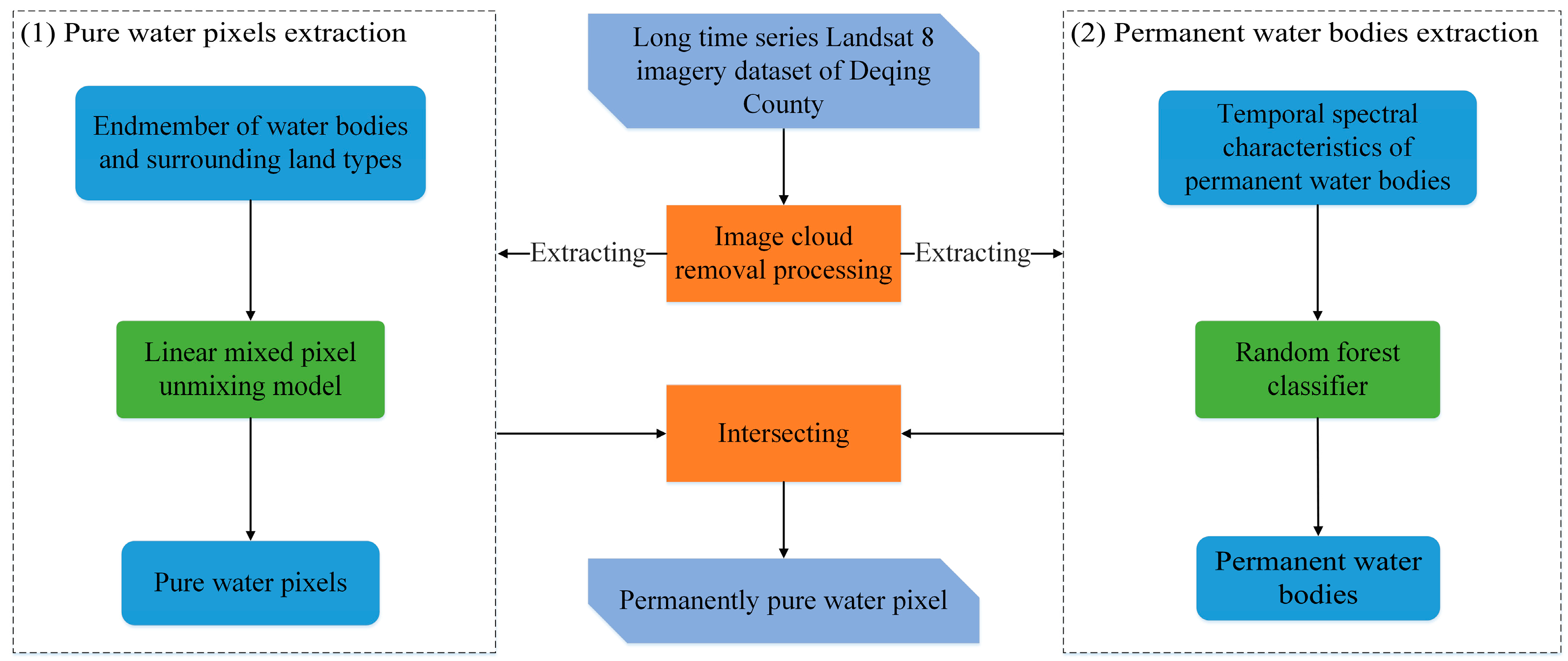
When utilizing this data for classification research, it is necessary to mask out unnecessary observation conditions, such as sunlight, clouds, land pixels, mixed pixels, and seasonal variations in rivers, etc. (Figure 2). The processing flow is as follows:
  • First, utilize the quality evaluation band that comes with the dataset, employing GEE’s built-in band logic operation function to perform cloud removal from the images.
  • Through the mixed pixel decomposition method, mixed pixels with mixed features are removed to extract relatively pure water pixels. Mixed pixels contain multiple features, which makes it difficult for classifiers to decide which category to assign them to, thus lowering the accuracy of classification results [31,39]. The impurity of the pixel features interferes with data statistics and analysis, making it difficult to accurately reflect the actual situation. By using mixed pixel decomposition techniques to eliminate mixed pixels, we extract purer water body pixels, which improves the accuracy and scientific validity of the subsequent classification results [40].
  • Permanent water bodies can be extracted using the time-spectral characteristics of surface features (periodic changes of spectral features in the time dimension) [41]. Seasonal changes in water bodies will cause some areas to alternate between water and land within a year, resulting in an extreme data imbalance, where some areas have less available data than other areas, affecting the accuracy of the SDG6.3.2 evaluation. By masking seasonal water bodies, this can be avoided, while also improving the accuracy of the evaluation results.

3. Methods

The technical route of this research is as follows (Figure 3): It mainly consists of three parts. First, the remote sensing water quality sample-enhancement method is used to collaborate with Landsat 8 data and station water quality-monitoring data to build a remote sensing water quality sample library under uncoordinated open-space conditions. This sample library is then used to build a random forest excellent water quality classification model. Finally, the SDG 6.3.2 pixel-based spatial evaluation method was designed, and the classification results were used for evaluation.

3.1. Remote Sensing Water Quality Sample-Enhancement Method for Synergizing Remote Sensing Data with Ground Monitoring Station Data

3.1.1. Remote Sensing Water Quality Sample Expansion Based on Rule Generation

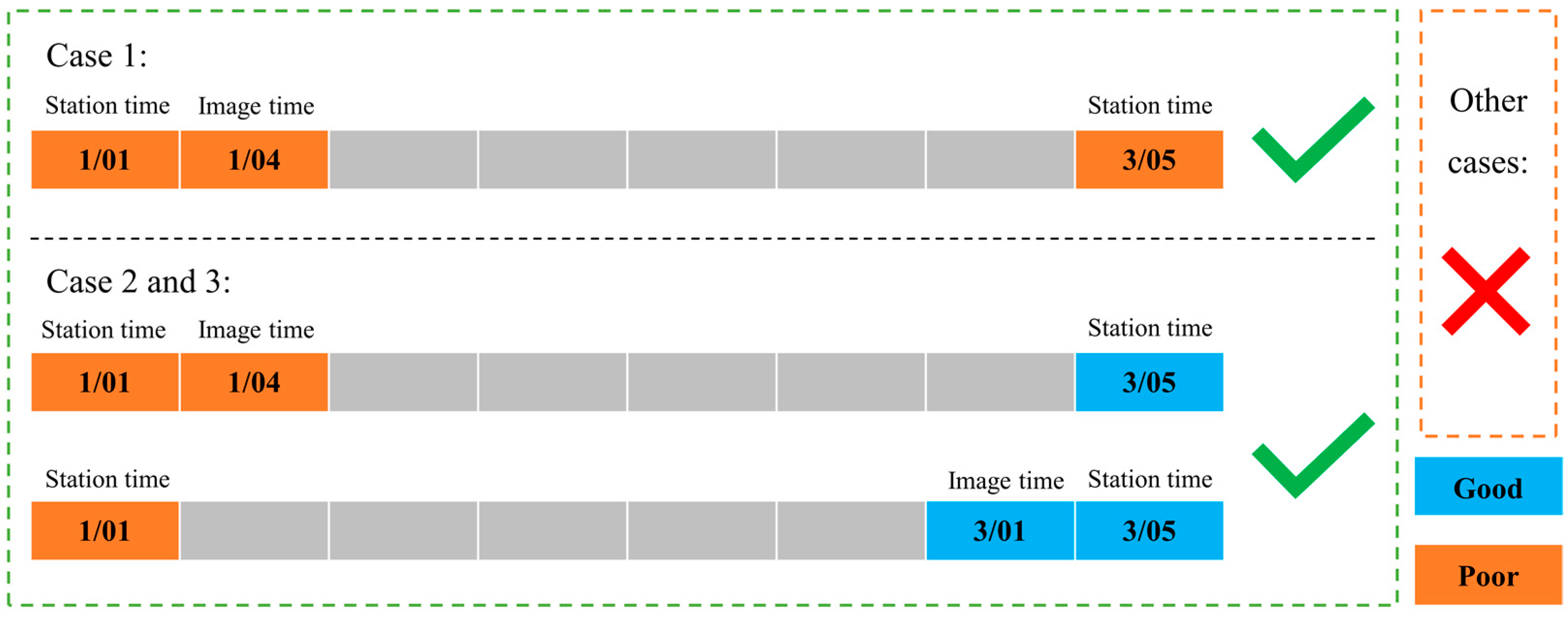
Water pollution is a persistent condition that may occur suddenly, but it often takes a long time for the pollution to dissipate. The degree (value) of pollution may change in adjacent time periods, but the pollution state will remain constant. Based on this scientific premise, we expand the temporal dimension of monitoring data sampling from a single point to a time window from 1 to 8 days before and after the sampling time. Subsequently, we match the two datasets (Figure 4) and establish the criteria (Figure 5) for retaining or discarding the matched data as follows:
  • Retain expanded sampling points when the water quality category of the sampling time points before and after the imaging time point is consistent;
  • If there is a change in the water quality category of the sampling time points before and after the imaging time point, and if the imaging time point is after the matched sampling time point and the water quality of the sampling time point is poor, retain the expanded sampling points;
  • If there is a change in the water quality category of the sampling time points before and before the imaging time point, and the imaging time point is after the matched sampling time point and the water quality of the sampling time point is good, retain the expanded sampling points;
  • In other cases, the expanded data will not be retained.
In the collection of the water quality data measured at the monitoring stations, which includes twenty-one parameters, seven commonly utilized parameters that can be directly or indirectly inferred through remote sensing techniques were selected. These include dissolved oxygen (DO), the permanganate index (CODMn), the dichromate index (CODCr), total phosphorus (TP), ammonia nitrogen (NH3-N), petroleum, and fluorides [36].
The measured values for each sample were classified according to the ‘Environmental quality standards for surface water’ (GB3838-2002). Water quality parameters meeting Class I to III standards were categorized as ‘Good’, while those failing to meet these standards were categorized as ‘Poor’. The water quality category is determined with the ratio of the number of good parameters to the total number of parameters, with a threshold of 80%. If 80% or more of the parameters meet the standard, the water quality is considered ‘Good’ and assigned a value of ‘1’. Otherwise, it is classified as ‘Poor’ and assigned a value of ‘0’.

3.1.2. Sample Augmentation Dataset Optimization Based on Anomaly Detection

On one hand, due to potential errors in field sampling and laboratory analyses, the accuracy and precision of the collected field data might be compromised [13]. On the other hand, despite the existence of screening rules, there remains a slight possibility that the expanded point water quality category may not align with the actual water quality category. Given these two considerations, it is essential to perform outlier removal on the expanded sample dataset. Firstly, a good water quality sample must be a relatively isolated presence in a collection of bad water quality samples, and vice versa. Secondly, through our preliminary screening, there should be very few inconsistencies between the water quality sample categories and the actual categories. Therefore, this paper will utilize the isolated forest outlier detection method.
Isolation Forest [42] is an unsupervised machine learning algorithm used to detect outliers. It constructs a random tree, and measures the degree of anomalous data points based on their path length within the tree. Since anomalies typically require fewer splitting steps to isolate, Isolation Forest can identify outliers relatively quickly [43]. It is well suited for high-dimensional data, and can efficiently identify outliers in a short period [44]. When using this method, it is crucial to adjust the ‘contamination’ parameter to accurately reflect the proportion of outliers present. This will ensure stable algorithm performance, particularly on small-scale datasets.
In this study, the Isolation Forest algorithm from the Python sklearn library is utilized for conducting outlier detection on a sample dataset expanded, based on predefined rules and categorized by water quality, followed by the computation of outlier detection scores. The sklearn implementation of the Isolation Forest algorithm incorporates a modification to the anomaly score, where outliers are typically represented by negative scores, indicating that lower scores correspond to greater anomalies. Herein, we aim to refine the dataset by targeting the removal of the bottom 10% of data based on the outlier detection scores, thereby optimizing the dataset for subsequent analyses.

3.2. Water Quality Classification Feature Selection and Model

3.2.1. Construction and Selection Methods of Feature Variables

Based on existing research results [15,45], this study fully utilizes information from various bands. The construction of classification features mainly includes four parts (Table 1). The first part consists of eight spectral bands from Landsat 8, namely B1, B2, B3, B4, B5, B6, B7, and B10. The second part includes 28 features representing the band differences of these eight bands. The third part comprises 28 features representing the band ratios of the eight bands. Lastly, the fourth part includes 28 features representing the normalized band ratios of the eight bands.
Conducting correlation analysis between water quality parameters and characteristic parameters is crucial to identify characteristics with significant correlations. Although building a comprehensive set of feature parameters can improve accuracy to a certain extent, too many such parameters may lead to information redundancy, negatively affecting the efficiency and accuracy of the classification model [46]. This article adopts three methods of feature parameter selection and combination as follows:
  • Random forest sampling: This approach generates multiple decision trees to classify objects sequentially. The aggregated result of each decision tree’s classification contributes to the final category predicted by the random forest, thereby improving the classification accuracy. This process also evaluates the importance of different features bing involved in the classification [47,48]. Features whose cumulative weight are in the top 60% are selected;
  • ReliefF feature selection: The ReliefF method is used for feature selection [49,50]. It starts by randomly selecting a sample, R from all training samples, then extracting k nearest neighbors from samples within the same category as R. For samples in different categories from R, k nearest neighbors are also selected. The feature’s classification ability is determined by calculating the maximum distance moved by samples of the same and different categories. Features with higher weights are considered more significant in classification. The top 60% of features, whose cumulative weight is reached, are chosen.;
  • Pearson correlation coefficient: Use the Pearson correlation coefficient to screen feature parameters [51]. Calculate the person correlation coefficient between each characteristic parameter and the water quality parameter [52]. The larger the absolute value of the Pearson correlation coefficient, the stronger the correlation between the two [53]. Among the correlation coefficients between water quality parameters and features, the top ten features among each water quality parameter are selected as feature variables.
By applying these selection methods, the study aims to balance the trade-off between including sufficient feature parameters for accurate classification and avoiding redundancy that can degrade model performance.

3.2.2. Model Construction

The random forest (RF) algorithm, a cornerstone in ensemble machine learning, finds extensive application across various image classification domains [54,55]. As a classical model, RF operates through a collection of numerous classification and regression trees, each weighing the importance of variables, which are identifiable post training. RF integrates bagged ensemble learning and stochastic sub-space methodologies, facilitating a comprehensive analysis of variable characteristics within the training dataset. RF boasts considerable advantages over alternative algorithms, displaying a robust performance. Its unbiased estimation ensures excellent model generalization [56]. Numerous studies have validated RF’s effectiveness in tackling nonlinear challenges and processing high-dimensional data in remote sensing image classification, establishing it as a potent solution in the field [57,58,59,60].
In this study, the random forest classifier provided on the Google Earth Engine platform was used to train the model using eight input datasets, and the model with the best performance was selected. These datasets are combinations of the constructed sample sets from 5 days and 8 days around the sampling event, along with various feature variable groups. The number of regression trees within the random forest classifier is a critical parameter when defining the RF model structure. After extensive experimentation and optimization, this number was set to 300. Other parameters were kept at their default values.

3.2.3. Accuracy Evaluation Method

Stratified k-fold cross-validation is an enhanced variant of k-fold cross-validation, particularly beneficial for datasets with imbalanced classes [61,62]. This study employs stratified k-fold cross-validation with the k set to 10, dividing the data into 10 mutually exclusive subsets. Sequentially, one subset is chosen as the validation set, and the remaining nine subsets serve as the training set to train the model. The discrepancies between the field measurement data and the model data are evaluated using a confusion matrix along with various statistical indicators. The average of the 10 performance evaluation metrics serves as the final performance evaluation of the model. The formulas for calculating the overall accuracy (OA) and Kappa coefficient are as follows:
O A % = i = 1 n P i i N × 100 %
K a p p a = N i = 1 n P i i i = 1 n P i + × P + i N 2 i = 1 n P i + × P + i
where n is the number of categories; N is the total number of validation samples; Pii is the number of correctly classified samples for each category, found on the diagonal of the confusion matrix; Pi+ is the total number of samples classified into a category by the classifier; and P+i is the total number of validation samples for a category.

3.3. Sustainable Development Goal 6.3.2 Evaluation Using Remote Sensing Water Quality Classification Results

3.3.1. Constructing Water Body Unit to Support Evolution

UN-Water defines a water body as a distinct portion of surface water that is considered relatively independent, typically classified as lakes or river segments delineated by endpoints or nodes. However, applying this definition directly to Deqing County is challenging due to its complex water system and sparse monitoring stations. In this study, we delineate water body units in Deqing County based on the connotation of water bodies, aiming to maintain consistency with UN-Water’s SDG 6.3.2 Tier 2 monitoring method in terms of the scale in subsequent studies [63]. By definition, a water body unit should also be a relatively independent area.
Considering the spatial distribution and source characteristics of the water system in Deqing County, it is divided into two major basins: the Dongtiaoxi River Basin and the Beijing-Hangzhou Grand Canal Basin, and further subdivided into various water body units within these basins (Figure 1). Most water bodies in the Dongtiaoxi River Basin are natural, and can be clearly delineated using DEM analysis for river flow direction, with delineation based on river nodes, tributaries, and the presence of water quality-monitoring stations.
The Beijing-Hangzhou Grand Canal Basin, which is characterized by a dense network of waterways, including many artificial canals, complicates the application of the previous delineation method. In this basin, numerous polders are artificially delineated and separated by sluices and locks, resulting in limited water exchange and flow between them, so that each polder approximates a semi-independent river network system [64]. Water body units in this catchment can first be subdivided on the basis of major watercourses, followed by a secondary subdivision on the basis of polder dikes. Units without water quality-monitoring stations are merged with adjacent units with stations, and efforts are made to keep monitoring stations away from unit boundaries to better represent water quality. It is important to ensure that each unit contains at least one monitoring station per year, as monitoring station locations change over the years.

3.3.2. Evaluation Plan Design

This study draws on the SDG 6.3.2 evaluation methodology provided by UN-Water to establish a simplified, universally applicable, pixel-based SDG 6.3.2 evaluation scheme from a remote sensing perspective as follows (Figure 6) [6]:
  • For long-term series data for a given pixel, if the standard time ratio (i.e., duration of good water quality/total duration) exceeds 80 percent, the water quality for that pixel is classified as good for the monitoring period;
  • For the long-term series data of a specific water body, if the proportion of good quality water pixels (number of good quality pixels/total number of pixels) exceeds 80%, then the water quality of that water body is considered good during the monitoring period. The water quality score for the water body = (number of good quality pixels/total number of pixels) * 100;
  • For the long-term series data of a certain area (e.g., a watershed or lake district), if the average water quality score of all contained water bodies exceeds 80, then the water quality of that area is considered good during the monitoring period;
  • For the long-term series data of a certain region, if the average water quality score of all included areas exceeds 80, then the water quality of that region is considered good during the monitoring period.
This framework provides a structured approach for evaluating water quality across different scales using remote sensing data, thus facilitating the evaluation of compliance with SDG 6.3.2 targets.

4. Results

4.1. Sample Enhanced Statistical Results

The sampling times were selected to extend from 1 day before and after the sampling time to 8 days before and after the sampling time. A total of eight time windows were used to extend the water quality samples of collaborative remote sensing data and ground monitoring station data (Table 2). It can be seen that there are only six sampling dates that match the acquisition time of the remote sensing data and the sampling time of the ground monitoring data. However, the time window for matching the ground monitoring data is gradually expanded, and the number of collected samples increases significantly. When the sampling time of the ground monitoring stations was extended to the time window of eight days before and after, the number of sample data in the sample set reached 144. Considering the balance between the two categories of samples, the 5 days before and after and the 8 days before and after datasets were selected as the final results and entered into the next step.
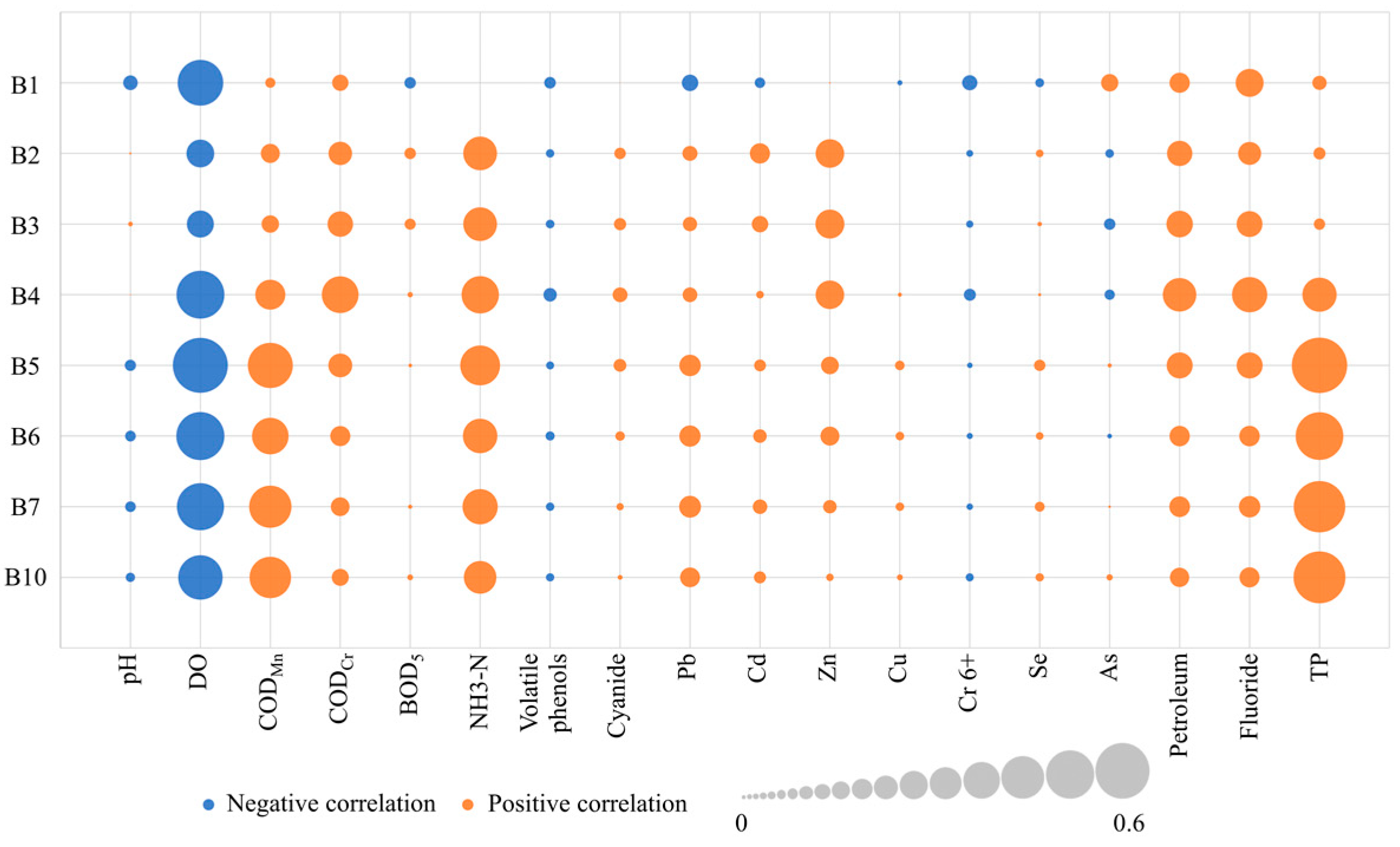
Meanwhile, in the correlation analysis results between the water quality parameters and remote sensing image band features (Figure 7), it was found that the water quality parameters associated with features with higher correlation are generally consistent with the seven selected water quality parameters. This is consistent with existing research and knowledge. It indicates that the extended sample set still retains the original water quality remote sensing feature information, which validates the feasibility of our extension method.

4.2. Construction of Feature Variables

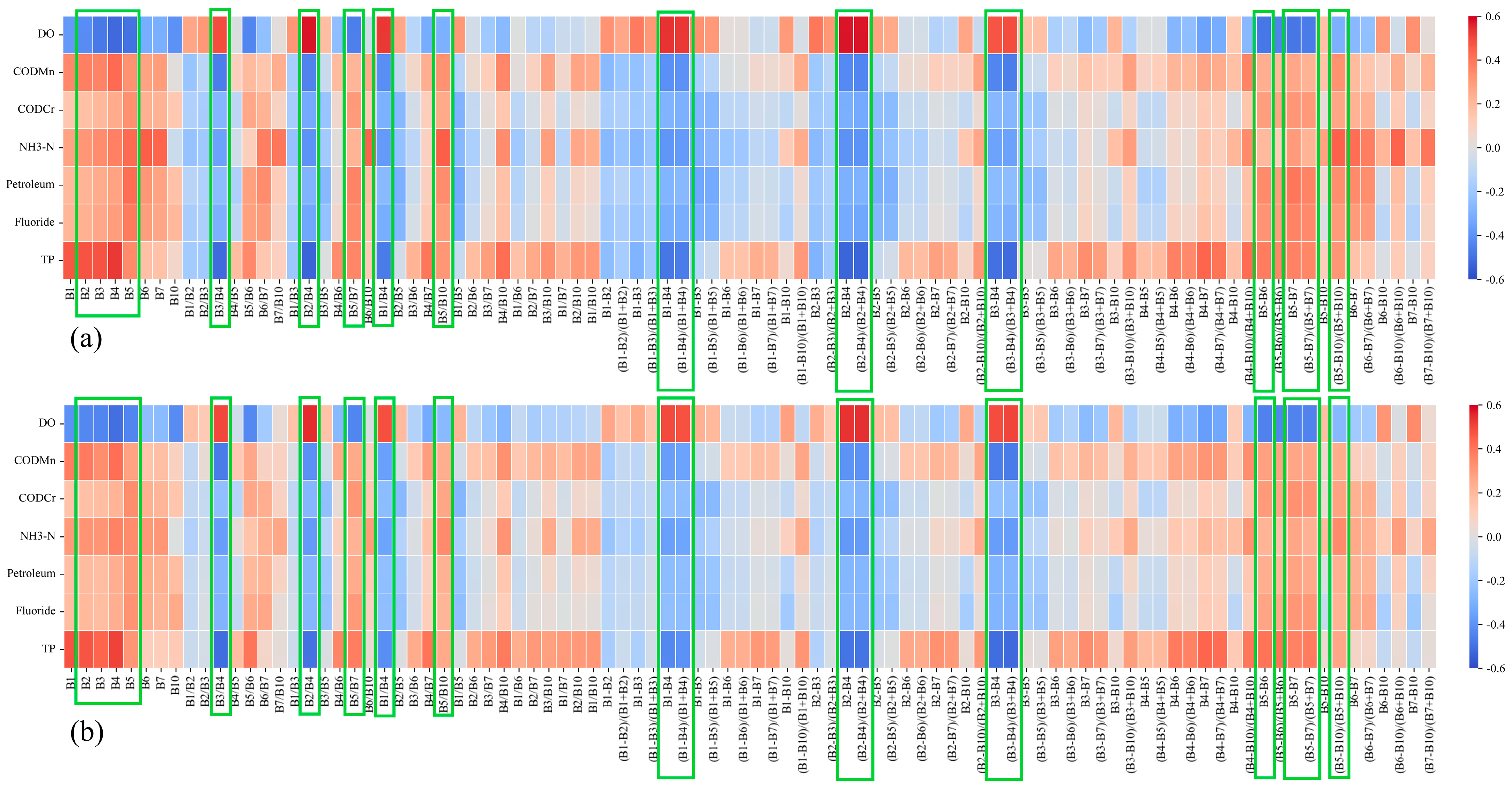
Based on the results of the sample expansion, feature optimization was performed separately on the datasets for ±5-day and ±8-day time windows. In addition, the raw expanded datasets, which were expanded during the sampling process but not optimized, were used for a control experiment. The results of the feature selection used two approaches, the random forest feature importance evaluation and the ReliefF filter-based feature selection method (Figure 8). By performing correlation analysis on the spectral bands and water quality parameters of the ±5-day and ±8-day datasets before and after, it was found that the Pearson correlation of the two datasets has a strong similarity (Figure 9). Therefore, consistent feature variables are used. Pearson correlation feature combinations include the following: B2/B4, B2 − B4, (B2 − B4)/(B2+B4), B1/B4, B1 − B4, (B1 − B4)/(B1 + B4), (B3 − B4)/(B3 + B4), B5, B3/B4, B5 − B6, (B5 − B10)/(B5 + B10), B5/B7, B3 − B4, B5 − B7, (B5 − B7)/(B5 + B7), B4, B5/B10, B2, B3. Finally, four sample sets with a total of sixteen combination solutions were obtained (Table 3).

4.3. Model Training Results and Accuracy Verification

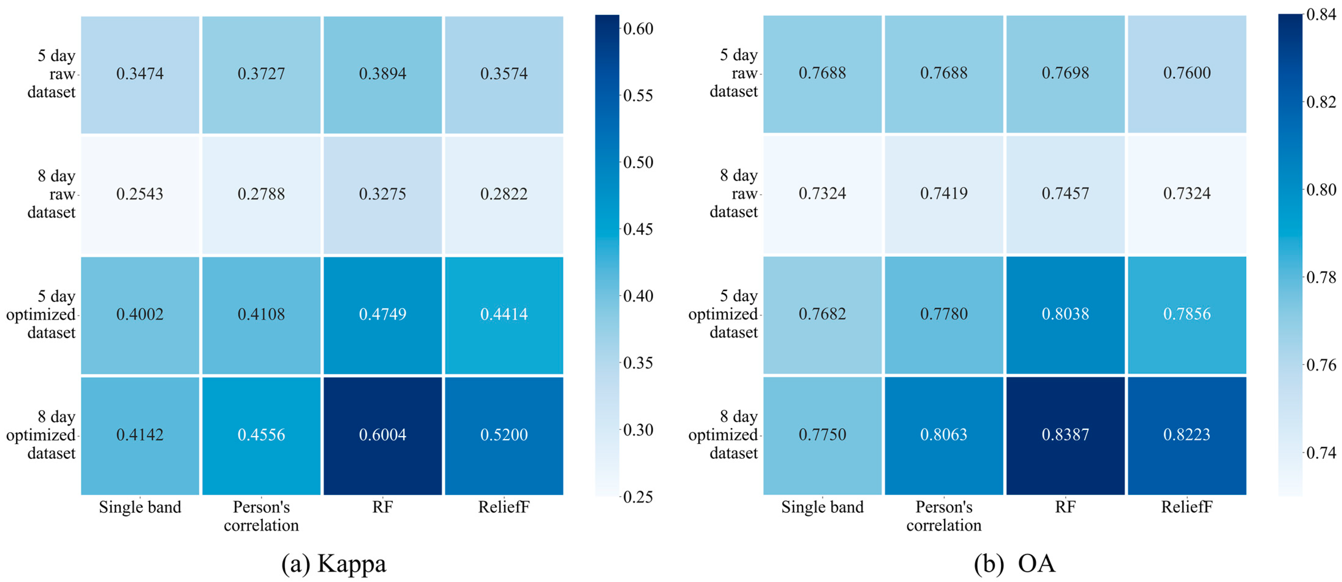
Judging from the overall classification accuracy and Kappa coefficient (Figure 10), the overall accuracy and Kappa changes caused by the different combinations of feature variables between the 5-day original dataset and the 8-day original dataset are very small. However, the datasets processed for outliers show improvements in both aspects. Both the 5-day and 8-day optimized datasets show significant improvements in the overall accuracy and kappa coefficient over the original dataset across different feature combinations.
A longitudinal comparison of the datasets shows that outlier removal significantly improves the overall classification accuracy and Kappa coefficient of the sample datasets. The 8-day raw dataset exhibited the lowest overall accuracy and Kappa coefficient, but after the outlier removal, it became the highest of the four datasets. Although the 5-day raw dataset was superior to the 8-day raw dataset in both the overall classification accuracy and Kappa coefficient, the 5-day optimized dataset did not perform as well as the 8-day optimized dataset. This discrepancy can be attributed to the fact that the 5-day raw dataset had fewer anomalies than the 8-day raw dataset, meaning that the quality of the 5-day raw dataset was superior. After the outlier removal, the difference in anomalies between the two datasets decreased significantly, but the 5-day optimized dataset (112 data points) had fewer data points when compared to the 8-day optimized dataset (144 data points). As a result, the 5-day optimized dataset was inferior to the 8-day optimized dataset in terms of the overall classification accuracy and Kappa coefficient.
A horizontal comparison of feature combinations shows that combinations that underwent feature optimization had higher overall accuracy and Kappa coefficients when compared to direct single-band combinations. In particular, the feature combinations selected by the random forest feature importance evaluation method achieved the highest overall classification accuracy and Kappa coefficient, reaching 0.8387 and 0.5004, respectively, followed by the ReliefF method and the Pearson correlation coefficient method.
In summary, the optimization methods for expanding the datasets have screened and removed outliers, thereby improving the quality of the dataset, while the feature prioritization methods have extracted more useful variables for classification. This demonstrates the feasibility and scientific value of the dataset expansion and optimization methods proposed in this study. Both the expanded dataset optimization method and the feature selection approach contribute significantly to improving the accuracy of the classification models.

4.4. Spatiotemporal Pattern of Water Quality in Deqing County

Through the statistical analysis of water quality classification results at the pixel scale for Deqing County from 2013 to 2022 (Figure 11), it was found that the water quality in Deqing County showed an improving trend from 2013 to 2015. In 2013, only 60.25% of the water body pixels were classified as having good water quality. By 2014, this proportion increased by 13.65% to 76.9%, and, in 2015, 83.16% of the water body pixels achieved good water quality. Subsequently, from 2015 to 2022, the proportion of water body pixels classified as good quality remained stable, maintaining above 80%.
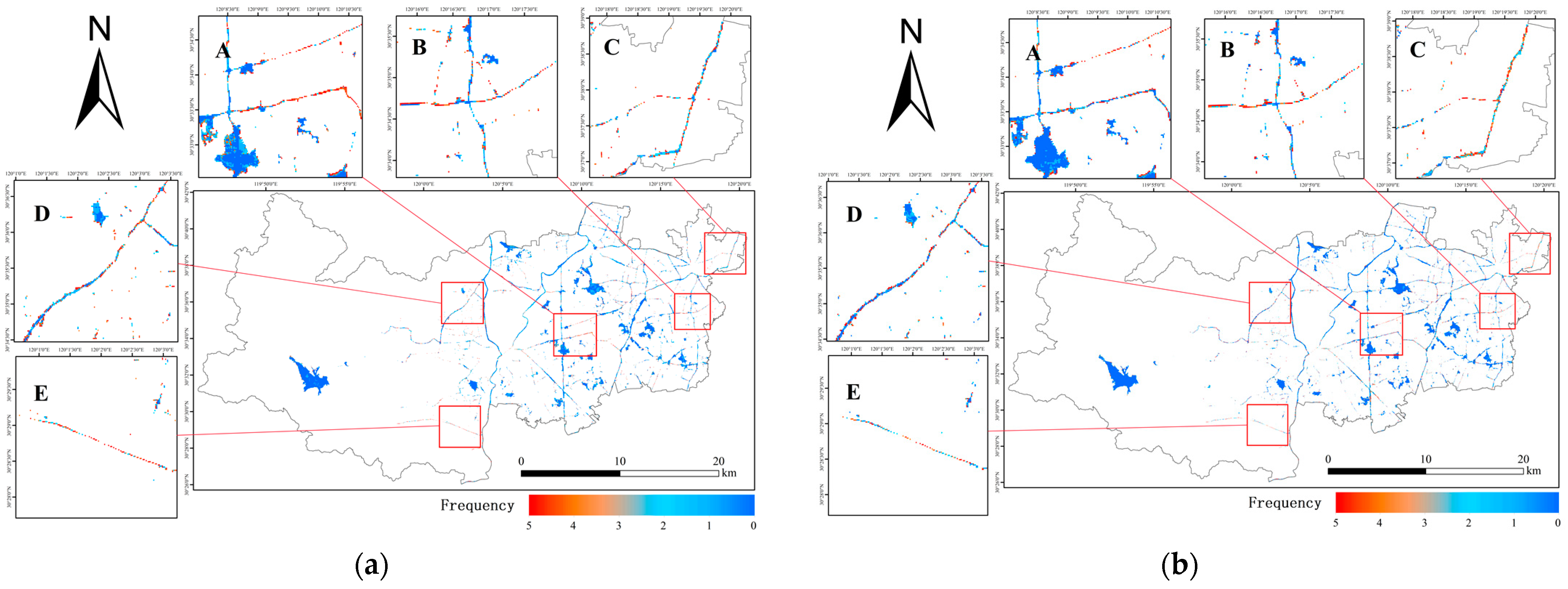
After aggregating the water quality classification results at the pixel scale for Deqing County from 2013 to 2022 and after conducting spatial analysis (Figure 12), it is observed that, when compared to the main rivers and lakes, the tributaries in the central and western parts of the county have a higher distribution of poor-quality water pixels. In the period from 2013 to 2017 (Figure 12a), most of the main rivers, lakes, and tributaries exhibited varying degrees of water pollution. However, from 2018 to 2022 (Figure 12b), the water quality of the main rivers and lakes (areas A, D, E) showed significant improvement, and most of the tributaries and smaller water bodies (areas A, D, E) also experienced varying degrees of improvement. In contrast, the water quality in the eastern part of Deqing County (areas B, C), especially the northeastern corner region (areas C), did not show significant changes in either time period.
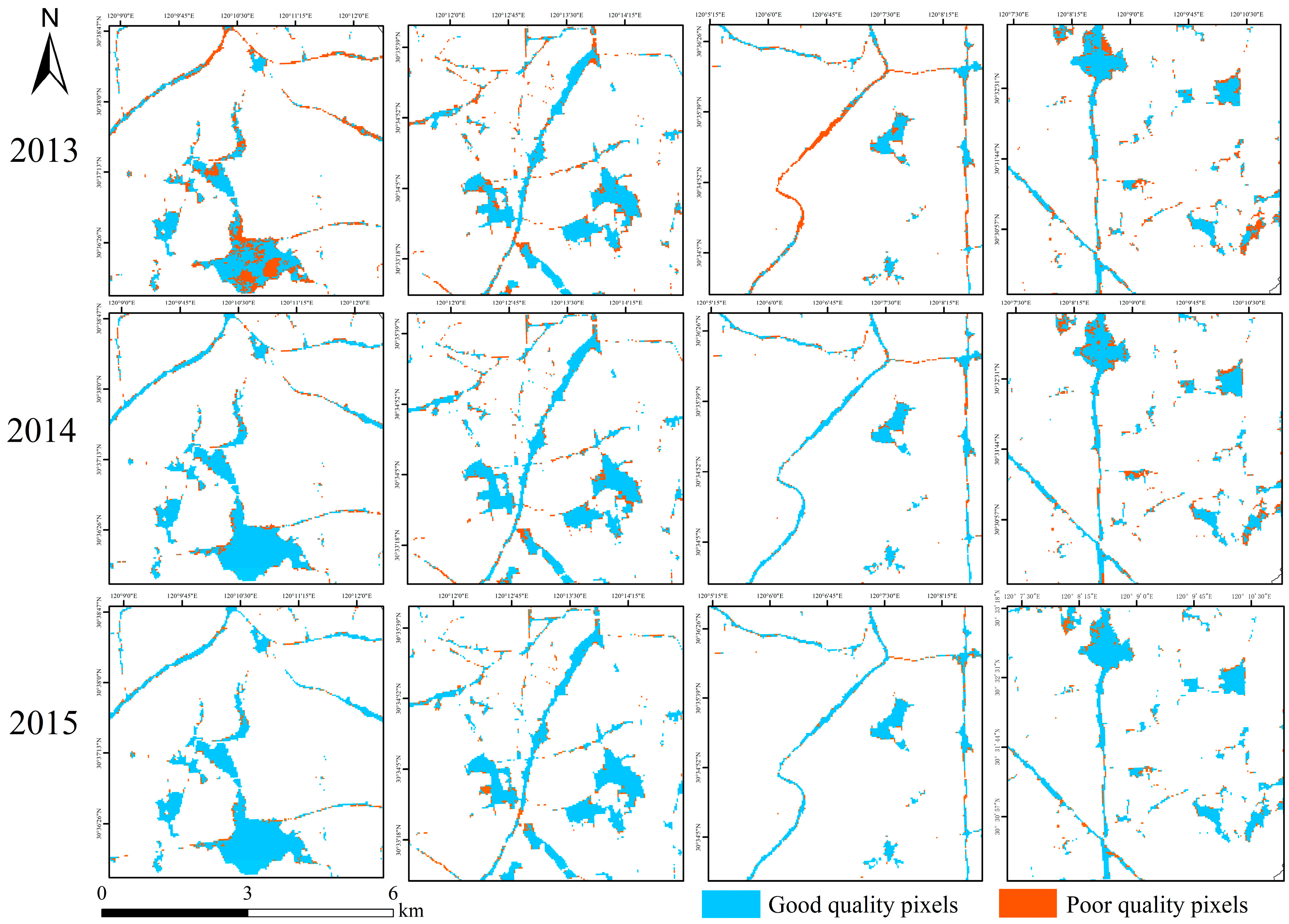
Further temporal and spatial analysis (Figure 13) reveals that, in 2013, except for the western mountainous areas where the water quality was good, other regions of Deqing County experienced various degrees of water pollution, indicating a severe situation. By 2014, there was a significant overall improvement in water quality, particularly in the main rivers where the condition of water quality was noticeably enhanced, and the number of poor water body pixels had substantially decreased. Lakes and tributaries also show varying degrees of improvement. In 2015, the water quality further improved, with visible enhancements in the lakes and tributaries. Over the following seven years, the water quality remained stable, with no significant changes.

4.5. Deqing County Water System SDG 6.3.2 Evaluation

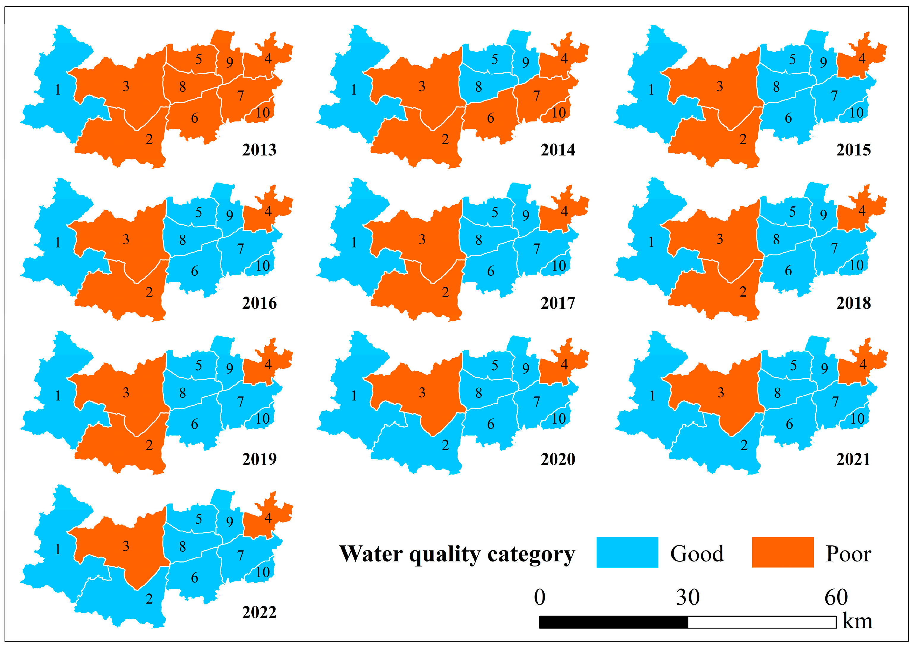
This article uses the pixel-based SDG 6.3.2 evaluation method to evaluate Deqing County, and the results are shown in Figure 14 and Figure 15. At the regional scale, the SDG 6.3.2 score (81.63) of Deqing County reached a good level since 2015, and then maintained a stable state. At the watershed scale, the evaluation scores of RGB1 are slightly higher than those of RGB2, which means that the water quality condition of RGB1 is better than that of RGB2. At the same time, the evaluation score curves of the two are similar, indicating that the water quality changes in the two watersheds in Deqing County are relatively uniform. Furthermore, the results of the water body unit scale evaluation indicate that the water quality of Deqing County has improved significantly between 2013 and 2015, and then maintained a stable improvement trend, and that, by 2022, all of them have reached a good level, except for area 3 in the center and area 4 in the northwest corner.

5. Discussion

Current remote sensing studies on water quality focus on inverting water quality parameters. However, water quality parameters in water bodies are constantly changing in time and space, requiring a high degree of temporal and spatial synchronization between satellite remote sensing data and ground data. It is often necessary to spend a significant amount of money on field sampling to obtain more air–ground spatiotemporal synchronization data before conducting a study. However, interpreting SDG 6.3.2 reveals that the indicator is only concerned with whether the water quality is good or not, rather than the values of individual water quality parameters. Under a real situation, decisionmakers and the general public are primarily concerned with whether the water is polluted or not, rather than the individual water quality parameters, including SDG 6.3.2. Therefore, we simplify the complex process of quantitative inversion and the comprehensive evaluation of multiple water quality parameters into a simple qualitative dichotomous classification process for conventional water quality classification. Pollution is a persistent condition that can occur suddenly but does not disappear suddenly. This also reduces the requirement for satellite remote sensing data and ground data to be highly synchronized in time. Based on this, this paper proposes a method for enhancing remote sensing water quality samples. The method involves expanding the time window for matching the two datasets until a sufficient amount of data is obtained. By establishing correlation rules and outlier detection methods, this method removes abnormal data to ensure data quality and constructs a water quality classification model. This approach maximizes the use of existing data, saves human resources and time costs as compared to existing water quality studies, and is more suitable for practical applications.
Moreover, the proposed classification model of water quality in this paper can synthesize all remote sensing-reflected water quality parameters. In this classification model, the relationship between each water quality parameter in the sample and the water quality category is determined by the surface water environmental standards. The number of good water quality parameters determines whether the water quality sample is good or not. Most studies on water quality monitoring using remote sensing focus on medium and large rivers and lakes, and there are no mature evaluation results for comparative validation. This paper focuses on Deqing County, a representative of typical inland small and medium-sized urban river systems. The study area presents more challenges for remote sensing-based water quality monitoring than other water systems. Deqing County has mature SDG 6.3.2 water quality evaluation results that can be compared and verified with the evaluation results presented in this paper.
Upon comparing the evaluation results presented in this paper with the existing evaluation results of Deqing County, a high degree of similarity is observed. This similarity demonstrates the objectivity and accuracy of the evaluation method employed in this paper. In analyzing the water quality situation in Deqing County by combining the results of water quality classification and evaluation, we discovered that the change in water quality can be divided into two phases. The first phase, from 2013 to 2015, showed significant improvement, while the second phase, from 2015 to 2022, showed stable fluctuation. Our findings are consistent with the background of water governance in Deqing County. In 2013, Deqing County began implementing the ‘five water governance’ program to rectify water quality pollution. By 2015, the program had been highly successful. At the same time, the measured data at the monitoring site also support this result (Table 4). It can be seen from the table that the annual average values of five water quality parameters in 2013 were hovering near the target values. Among them, the average values of CODCr and NH3-N did not reach the target value. In 2014, there were still three water quality parameters that were very close to the target values. Among them, the average value of NH3-N did not reach the target value. By 2015, the water quality had improved considerably, with all water quality parameters far better than the target values. The water quality situation has remained stable since then. In 2020, due to the COVID-19 pandemic, human production and operation activities were halted, resulting in the further restoration of river water quality and a peak in the water quality situation (the ratio of good water body pixels reached 84.6%, and the SDG 6.3.2 spatial type evaluation value reached 83.4). In the following two years, despite the recovery of human activities and the impact of drought, the water quality declined. However, the proportion of good water body pixels and the SDG6.3.2 spatial type evaluation value remained above the good level, respectively, and there was little change overall. The evaluation results indicate that, while the overall water quality in Deqing County has reached a good status since 2015, there are still certain water quality problems in areas No. 2, No. 3, and No. 4. Particularly in the No. 4 area, the water quality situation did not improve significantly over the past decade. We further analyze the causes based on the actual situation. The majority of Deqing County’s center is situated in area 3, with a small portion located in area 2. These areas experience frequent human activity, making water quality management more challenging than in other regions. Area 2 comprises a small portion of the central town. Thanks to advancements in water quality management, the overall water quality of area 2 reached a good level in 2020. The poor water quality in area 4 is due to its border with neighboring counties and the fact that some of the water flows in from the adjacent area. The water quality conditions in area 4 are affected not only by the production and life in the region, but also by the poor water quality conditions in the neighboring counties. Therefore, effective water management requires joint efforts between the two areas, and relying solely on No. 4 area is not sufficient.
In summary, using the remote sensing water quality sample enhancement method applied to water quality classification proposed in this study for the construction of water quality models can make full use of the existing data already available. It saves a lot of human resources and time costs, while ensuring data quality, which is more suitable for application in practical work. At the same time, using this model to evaluate SDG 6.3.2 results in a more comprehensive reflection of multiple water quality parameters, better representing the actual water quality situation. This approach saves time and cost while ensuring the accuracy and reliability of the evaluation results. It significantly enhances the efficiency of SDG 6.3.2 assessment, while reducing the threshold for evaluation.
Currently, remote sensing is limited in its ability to monitor and evaluate water quality due to its inability to detect water quality parameters that lack significant optical properties, such as metallic pollutants. The pollution parameters for water quality in Deqing County, the study area for this research, are primarily reflected by remote sensing. These parameters include DO, CODMn, ammonia nitrogen, and total phosphorus. It is possible that there is heavy metal pollution and other types of pollution that cannot be detected via remote sensing in areas that are classified and evaluated as good. This is an important consideration when applying the method used in this study to other areas. However, when considering the causes of water pollution, it is important to note that agricultural and domestic water usage currently accounts for 80% of global fresh water usage [65]. Furthermore, water pollution is primarily caused by agricultural production and domestic water sources. [66] The main parameters of water pollution are total phosphorus (TP), ammonia nitrogen (NH3-N), and dissolved oxygen (DO) [67,68]. Therefore, the methodology used in this study has strong general applicability. Furthermore, previous research has been conducted on the remote sensing monitoring of heavy metal pollution in water quality. It is believed that this limitation will be effectively addressed in the future [69,70,71]. It should be noted that there is still a lack of a globally harmonized and fixed standard for water quality parameters, and local water quality standards need to be used for practical applications.

6. Conclusions

Based on Landsat 8 data and station water quality-monitoring data, a remote sensing water quality sample enhancement method under open-ground uncoordinated conditions was proposed in the field of water quality classification, and a random forest excellent water body classification model was constructed. The water quality distribution map of Deqing County was drawn to evaluate SDG 6.3.2 water quality indicators. First, according to the characteristics of water quality pollution, a remote sensing water quality sample enhancement method was proposed in the field of quality classification. By expanding the sampling time points of station data into time periods, the number of samples matched with Landsat 8 data increased, and the sample quality is ensured through reconstructing relevant rules and outlier detection. Experimental results confirmed that the enhanced sample set’s band-to-water quality parameter correlations align with existing research, verifying the method’s scientific validity and feasibility. Secondly, a random forest excellent water body classification model was constructed, and combined with Landsat 8 data, the water quality distribution map of Deqing County, China, from 2013 to 2022 was drawn. It was found that excellent water body classification models have a certain accuracy. The classification results show that the water quality in Deqing County improved significantly from 2013 to 2015, and then maintained stable fluctuations. From 2013 to 2015, the order of water quality improvement was roughly main rivers, lakes and tributaries. And poor water quality persists along the western border. These are consistent with the actual situation, which illustrates the scientificity and feasibility of the remote sensing water quality sample enhancement method we proposed. Finally, based on the results of excellent water body classification, a set of spatial evaluation methods was designed to evaluate SDG 6.3.2 indicators. It was found that Deqing County has generally maintained good water quality since 2015 (overall evaluation score >80%), but poor water quality still exists in the central urban areas and western border areas (the proportion of water body pixels with good water quality is <80%). It is recommended that relevant departments continue to strengthen the water quality supervision and management of small water bodies, and, at the same time, start from the external environment and strive to mobilize adjacent areas for collaborative management to improve the external environment of water quality in the region, achieving the sustainable development of water resources. This study demonstrates the examples and feasibility of using satellite data to support SDG 6.3.2 water quality reporting. At present, remote sensing technology still has shortcomings in detecting heavy metals in water. Given that global water pollution sources mainly come from agricultural and domestic sewage, which mainly affects parameters such as DO, TP, and NH3-N, the proposed spatial evaluation method based on remote sensing still has broad applicability. Future research aims to leverage multi-source remote sensing data to expand and refine the remote sensing water quality sample database, advancing towards fully automated SDG 6.3.2 evaluation processes.

Author Contributions

Conceptualization, H.C.; methodology, C.T., L.L. and H.C.; software, C.T.; validation, C.T. and H.C.; formal analysis, C.T., H.C., W.Y. and H.P.; investigation, C.T. and H.P.; writing—original draft preparation, C.T.; writing—review and editing, H.C., L.L., W.Y. and H.P.; visualization, C.T.; supervision, H.C.; project administration, H.C., H.P. and L.L.; funding acquisition, H.C., H.P. and L.L. All authors have read and agreed to the published version of the manuscript.

Funding

This research was supported by a grant from the National Natural Science Foundation of China (No. 41930650), the Hunan Provincial Natural Science Foundation of China (No. 2023JJ30232), the Hunan Provincial Natural Science Foundation of China (No. 2023JJ30236), and the Scientific Research Fund of Hunan Provincial Education Department (No. 22B0475).

Data Availability Statement

Restrictions apply to the availability of these data. Data were obtained from the Deqing County Environmental Protection Bureau and are available from the authors with the permission of the Deqing County Environmental Protection Bureau.

Acknowledgments

We are very grateful to the Deqing County Environmental Protection Bureau for providing station water quality-monitoring data. We wish to express our gratitude to NASA and GEE platform for providing rich computing resources.

Conflicts of Interest

The authors declare no conflicts of interest.

References

  1. Chen, J.Q. Global change and sustainable development of water resources. Adv. Water Sci. 1996, 7, 187–192. [Google Scholar]
  2. Lukhabi, D.K.; Mensah, P.K.; Asare, N.K.; Pulumuka-Kamanga, T.; Ouma, K.O. Adapted Water Quality Indices: Limitations and Potential for Water Quality Monitoring in Africa. Water 2023, 15, 1736. [Google Scholar] [CrossRef]
  3. Wang, Y.; He, W.; Chen, C.; Zhang, X.; Tang, H.; Li, P.; Tong, Y.; Li, M.; Lin, Y.; Yu, J.; et al. Different Countries Need Strengthen Water Management to Improve Human Health. J. Clean. Prod. 2022, 380, 134998. [Google Scholar] [CrossRef]
  4. United Nations Water. The United Nations World Water Development Report 2023: Partnerships and Cooperation for Water; United Nations Water: New York, NY, USA, 2023. [Google Scholar]
  5. United Nations. Transforming our World: The 2030 Agenda for Sustainable Development; United Nations: New York, NY, USA, 2015. [Google Scholar]
  6. United Nations Water. Integrated Monitoring Guide for SDG 6-Targets and Global Indicators; United Nations Water: New York, NY, USA, 2017. [Google Scholar]
  7. United Nations Water. Piloting the Monitoring Methodology and Initial Findings for SDG Indicator 6.3.2; United Nations Water: New York, NY, USA, 2018. [Google Scholar]
  8. Shen, M.; Duan, H.; Cao, Z.; Xue, K.; Qi, T.; Ma, J.; Liu, D.; Song, K.; Huang, C.; Song, X. Sentinel-3 OLCI Observations of Water Clarity in Large Lakes in Eastern China: Implications for SDG 6.3.2 Evaluation. Remote Sens. Environ. 2020, 247, 111950. [Google Scholar] [CrossRef]
  9. Adjovu, G.E.; Stephen, H.; James, D.; Ahmad, S. Overview of the Application of Remote Sensing in Effective Monitoring of Water Quality Parameters. Remote Sens. 2023, 15, 1938. [Google Scholar] [CrossRef]
  10. Qiu, R.; Wang, S.; Shi, J.; Shen, W.; Zhang, W.; Zhang, F.; Li, J. Sentinel-2 MSI Observations of Water Clarity in Inland Waters across Hainan Island and Implications for SDG 6.3.2 Evaluation. Remote Sens. 2023, 15, 1600. [Google Scholar] [CrossRef]
  11. Strobl, R.O.; Robillard, P.D. Network Design for Water Quality Monitoring of Surface Freshwaters: A Review. J. Environ. Manag. 2008, 87, 639–648. [Google Scholar] [CrossRef]
  12. Miao, J.; Song, X.; Zhong, F.; Huang, C. Sustainable Development Goal 6 Assessment and Attribution Analysis of Underdeveloped Small Regions Using Integrated Multisource Data. Remote Sens. 2023, 15, 3885. [Google Scholar] [CrossRef]
  13. Gholizadeh, M.H.; Melesse, A.M.; Reddi, L. A Comprehensive Review on Water Quality Parameters Estimation Using Remote Sensing Techniques. Sensors 2016, 16, 1298. [Google Scholar] [CrossRef]
  14. Topp, S.N.; Pavelsky, T.M.; Jensen, D.; Simard, M.; Ross, M.R.V. Research Trends in the Use of Remote Sensing for Inland Water Quality Science: Moving Towards Multidisciplinary Applications. Water 2020, 12, 169. [Google Scholar] [CrossRef]
  15. Odermatt, D.; Gitelson, A.; Brando, V.E.; Schaepman, M. Review of Constituent Retrieval in Optically Deep and Complex Waters from Satellite Imagery. Remote Sens. Environ. 2012, 118, 116–126. [Google Scholar] [CrossRef]
  16. Ahmed, W.; Mohammed, S.; El-Shazly, A.; Morsy, S. Tigris River Water Surface Quality Monitoring Using Remote Sensing Data and GIS Techniques. Egypt. J. Remote Sens. Space Sci. 2023, 26, 816–825. [Google Scholar] [CrossRef]
  17. Li, J.; Yu, Q.; Tian, Y.Q.; Becker, B.L.; Siqueira, P.; Torbick, N. Spatio-Temporal Variations of CDOM in Shallow Inland Waters from a Semi-Analytical Inversion of Landsat-8. Remote Sens. Environ. 2018, 218, 189–200. [Google Scholar] [CrossRef]
  18. Rahat, S.H.; Steissberg, T.; Chang, W.; Chen, X.; Mandavya, G.; Tracy, J.; Wasti, A.; Atreya, G.; Saki, S.; Bhuiyan, M.A.E.; et al. Remote Sensing-Enabled Machine Learning for River Water Quality Modeling under Multidimensional Uncertainty. Sci. Total Environ. 2023, 898, 165504. [Google Scholar] [CrossRef]
  19. Campbell, G.; Phinn, S.R.; Dekker, A.G.; Brando, V.E. Remote Sensing of Water Quality in an Australian Tropical Freshwater Impoundment Using Matrix Inversion and MERIS Images. Remote Sens. Environ. 2011, 115, 2402–2414. [Google Scholar] [CrossRef]
  20. Xie, Y.; Zhou, Q.; Xiao, X.; Chen, F.; Huang, Y.; Kang, J.; Wang, S.; Zhang, F.; Gao, M.; Du, Y.; et al. Satellite-Based Water Quality Assessment of the Beijing Section of the Grand Canal: Implications for SDG11.4 Evaluation. Remote Sens. 2024, 16, 909. [Google Scholar] [CrossRef]
  21. Ruben, G.B.; Zhang, K.; Bao, H.; Ma, X. Application and Sensitivity Analysis of Artificial Neural Network for Prediction of Chemical Oxygen Demand. Water Resour. Manag. 2018, 32, 273–283. [Google Scholar] [CrossRef]
  22. Zhou, Y.; Yu, D.; Yang, Q.; Pan, S.; Gai, Y.; Cheng, W.; Liu, X.; Tang, S. Variations of Water Transparency and Impact Factors in the Bohai and Yellow Seas from Satellite Observations. Remote Sens. 2021, 13, 514. [Google Scholar] [CrossRef]
  23. Wang, H.; Wu, M.A.; Zhou, Y.Y.; Xia, K.; Tang, Y.; Zhang, W. Influence of Field Environmental Factors on Water Transparency. Adv. Mater. Res. 2014, 1030–1032, 532–538. [Google Scholar] [CrossRef]
  24. Feng, L.; Hou, X.; Zheng, Y. Monitoring and Understanding the Water Transparency Changes of Fifty Large Lakes on the Yangtze Plain Based on Long-Term MODIS Observations. Remote Sens. Environ. 2019, 221, 675–686. [Google Scholar] [CrossRef]
  25. Kaya, Y.; Sanli, F.B.; Abdikan, S. Determination of Long-Term Volume Change in Lakes by Integration of UAV and Satellite Data: The Case of Lake Burdur in Türkiye. Environ. Sci. Pollut. Res. 2023, 30, 117729–117747. [Google Scholar] [CrossRef]
  26. Zhang, H.; Zhou, J.; Huangfu, K. Analysis on water quality monitoring indicators by remote sensing based on OLl data: A case of Huaihe River Basin in Xinyang City. Yangtze River 2021, 52, 47–53. [Google Scholar]
  27. Kolokoussis, P.; Karathanassi, V. Detection of Oil Spills and Underwater Natural Oil Outflow Using Multispectral Satellite Imagery. Int. J. Remote Sens. Appl. 2013, 3, 145–154. [Google Scholar]
  28. Vakili, T.; Amanollahi, J. Determination of Optically Inactive Water Quality Variables Using Landsat 8 Data: A Case Study in Geshlagh Reservoir Affected by Agricultural Land Use. J. Clean. Prod. 2020, 247, 119134. [Google Scholar] [CrossRef]
  29. Najafzadeh, M.; Basirian, S. Evaluation of River Water Quality Index Using Remote Sensing and Artificial Intelligence Models. Remote Sens. 2023, 15, 2359. [Google Scholar] [CrossRef]
  30. Choi, M.; Hur, Y. A Microwave-Optical/Infrared Disaggregation for Improving Spatial Representation of Soil Moisture Using AMSR-E and MODIS Products. Remote Sens. Environ. 2012, 124, 259–269. [Google Scholar] [CrossRef]
  31. Xiao, Y.; Chen, J.; Xu, Y.; Guo, S.; Nie, X.; Guo, Y.; Li, X.; Hao, F.; Fu, Y.H. Monitoring of Chlorophyll-a and Suspended Sediment Concentrations in Optically Complex Inland Rivers Using Multisource Remote Sensing Measurements. Ecol. Indic. 2023, 155, 111041. [Google Scholar] [CrossRef]
  32. Chen, S.; Hu, C.; Barnes, B.B.; Xie, Y.; Lin, G.; Qiu, Z. Improving Ocean Color Data Coverage through Machine Learning. Remote Sens. Environ. 2019, 222, 286–302. [Google Scholar] [CrossRef]
  33. Yang, L.; Driscol, J.; Sarigai, S.; Wu, Q.; Lippitt, C.D.; Morgan, M. Towards Synoptic Water Monitoring Systems: A Review of AI Methods for Automating Water Body Detection and Water Quality Monitoring Using Remote Sensing. Sensors 2022, 22, 2416. [Google Scholar] [CrossRef]
  34. Maťašovská, V.; Kothan, F.; Ledvinka, O.; Pumann, P.; Fojtík, T.; Makovcová, M.; Bendakovská, L. Využití metod dálkového průzkumu Země pro monitoring stavu koupacích míst. Vodohospodářské Tech. Ekon. Inf. 2021, 63, 37–45. [Google Scholar] [CrossRef]
  35. El Serafy, G.Y.H.; Schaeffer, B.A.; Neely, M.-B.; Spinosa, A.; Odermatt, D.; Weathers, K.C.; Baracchini, T.; Bouffard, D.; Carvalho, L.; Conmy, R.N.; et al. Integrating Inland and Coastal Water Quality Data for Actionable Knowledge. Remote Sens. 2021, 13, 2899. [Google Scholar] [CrossRef] [PubMed]
  36. Yang, H.; Kong, J.; Hu, H.; Du, Y.; Gao, M.; Chen, F. A Review of Remote Sensing for Water Quality Retrieval: Progress and Challenges. Remote Sens. 2022, 14, 1770. [Google Scholar] [CrossRef]
  37. Peterson, K.T.; Sagan, V.; Sloan, J.J. Deep Learning-Based Water Quality Estimation and Anomaly Detection Using Landsat-8/Sentinel-2 Virtual Constellation and Cloud Computing. GIScience Remote Sens. 2020, 57, 510–525. [Google Scholar] [CrossRef]
  38. Smith, V.H.; Joye, S.B.; Howarth, R.W. Eutrophication of Freshwater and Marine Ecosystems. Limnol. Oceanogr. 2006, 51 Pt 2, 351–355. [Google Scholar] [CrossRef]
  39. Zhao, D.; Lv, M.; Zou, X.; Wang, P.; Yang, T.; An, S. What Is the Minimum River Width for the Estimation of Water Clarity Using Medium-Resolution Remote Sensing Images? Water Resour. Res. 2014, 50, 3764–3775. [Google Scholar] [CrossRef]
  40. Lu, D.; Moran, E.; Batistella, M. Linear Mixture Model Applied to Amazonian Vegetation Classification. Remote Sens. Environ. 2003, 87, 456–469. [Google Scholar] [CrossRef]
  41. Duan, M.D.; Chen, H.; Peng, H.H.; Tan, C.M.; Xia, H.N.; Shi, Q. Seasonal wetlands extraction based on the typical characteristics of land and water alternation: A case study of East Dongting Lake. Remote Sens. Technol. Appl. 2024, 1–12. [Google Scholar]
  42. Liu, F.T.; Ting, K.M.; Zhou, Z.-H. Isolation Forest. In Proceedings of the IEEE International Conference on Data Mining, Pisa, Italy, 15–19 December 2008; pp. 413–422. [Google Scholar]
  43. Chabchoub, Y.; Togbe, M.U.; Boly, A.; Chiky, R. An In-Depth Study and Improvement of Isolation Forest. IEEE Access 2022, 10, 10219–10237. [Google Scholar] [CrossRef]
  44. Al Farizi, W.S.; Hidayah, I.; Rizal, M.N. Isolation Forest Based Anomaly Detection: A Systematic Literature Review. In Proceedings of the 2021 8th International Conference on Information Technology, Computer and Electrical Engineering (ICITACEE), Semarang, Indonesia, 23–24 September 2021; pp. 118–122. [Google Scholar]
  45. Papoutsa, C.; Akylas, E.; Hadjimitsis, D. Trophic State Index Derivation through the Remote Sensing of Case-2 Water Bodies in the Mediterranean Region. Open Geosci. 2014, 6, 67–78. [Google Scholar] [CrossRef]
  46. Guo, Q.L.; Li, J.L.; Guo, P. Extraction of Peanut Planting Area Based on Dual-temporal Remote Sensing Features of Crops. J. Appl. Meteorol. Sci. 2022, 33, 218–230. [Google Scholar]
  47. Breiman, L. Random Forests. Mach. Learn. 2001, 45, 5–32. [Google Scholar] [CrossRef]
  48. Genuer, R.; Poggi, J.-M.; Tuleau-Malot, C. Variable Selection Using Random Forests. Pattern Recognit. Lett. 2010, 31, 2225–2236. [Google Scholar] [CrossRef]
  49. Wang, Z.; Zhang, Y.; Chen, Z.; Yang, H.; Sun, Y.; Kang, J.; Yang, Y.; Liang, X. Application of ReliefF Algorithm to Selecting Feature Sets for Classification of High Resolution Remote Sensing Image. In Proceedings of the IEEE International Geoscience and Remote Sensing Symposium (IGARSS), Beijing, China, 10–15 July 2016; pp. 755–758. [Google Scholar]
  50. Urbanowicz, R.J.; Meeker, M.; La Cava, W.; Olson, R.S.; Moore, J.H. Relief-Based Feature Selection: Introduction and Review. J. Biomed. Inform. 2018, 85, 189–203. [Google Scholar] [CrossRef] [PubMed]
  51. Mei, K.; Tan, M.; Yang, Z.; Shi, S. Modeling of Feature Selection Based on Random Forest Algorithm and Pearson Correlation Coefficient. J. Phys. Conf. Ser. 2022, 2219, 012046. [Google Scholar] [CrossRef]
  52. Yigit Avdan, Z.; Kaplan, G.; Goncu, S.; Avdan, U. Monitoring the Water Quality of Small Water Bodies Using High-Resolution Remote Sensing Data. ISPRS Int. J. Geo-Inf. 2019, 8, 553. [Google Scholar] [CrossRef]
  53. Zhu, H.; You, X.; Liu, S. Multiple Ant Colony Optimization Based on Pearson Correlation Coefficient. IEEE Access 2019, 7, 61628–61638. [Google Scholar] [CrossRef]
  54. Dong, L.; Du, H.; Mao, F.; Han, N.; Li, X.; Zhou, G.; Zhu, D.; Zheng, J.; Zhang, M.; Xing, L.; et al. Very High Resolution Remote Sensing Imagery Classification Using a Fusion of Random Forest and Deep Learning Technique—Subtropical Area for Example. IEEE J. Sel. Top. Appl. Earth Obs. Remote Sens. 2020, 13, 113–128. [Google Scholar] [CrossRef]
  55. Zhang, T.; Su, J.; Xu, Z.; Luo, Y.; Li, J. Sentinel-2 Satellite Imagery for Urban Land Cover Classification by Optimized Random Forest Classifier. Appl. Sci. 2021, 11, 543. [Google Scholar] [CrossRef]
  56. Yu, R.; Zhang, K.; Ramasubramanian, B.; Jiang, S.; Ramakrishna, S.; Tang, Y. Ensemble Learning for Predicting Average Thermal Extraction Load of a Hydrothermal Geothermal Field: A Case Study in Guanzhong Basin, China. Energy 2024, 296, 131146. [Google Scholar] [CrossRef]
  57. Rodriguez-Galiano, V.F.; Chica-Olmo, M.; Abarca-Hernandez, F.; Atkinson, P.M.; Jeganathan, C. Random Forest Classification of Mediterranean Land Cover Using Multi-Seasonal Imagery and Multi-Seasonal Texture. Remote Sens. Environ. 2012, 121, 93–107. [Google Scholar] [CrossRef]
  58. Gislason, P.O.; Benediktsson, J.A.; Sveinsson, J.R. Random Forest Classification of Multisource Remote Sensing and Geographic Data. In Proceedings of the IEEE International Geoscience and Remote Sensing Symposium, Anchorage, AK, USA, 20–24 September 2004; Volume 2, pp. 1049–1052. [Google Scholar]
  59. Pal, M. Random Forest Classifier for Remote Sensing Classification. Int. J. Remote Sens. 2007, 26, 217–222. [Google Scholar] [CrossRef]
  60. Liu, Y.; Gong, W.; Hu, X.; Gong, J. Forest Type Identification with Random Forest Using Sentinel-1A, Sentinel-2A, Multi-Temporal Landsat-8 and DEM Data. Remote Sens. 2018, 10, 946. [Google Scholar] [CrossRef]
  61. Fontanari, T.; Fróes, T.C.; Recamonde-Mendoza, M. Cross-Validation Strategies for Balanced and Imbalanced Datasets. In Intelligent Systems; Xavier-Junior, J.C., Rios, R.A., Eds.; Springer International Publishing: Cham, Switzerland, 2022; pp. 626–640. [Google Scholar]
  62. Adagbasa, E.G.; Adelabu, S.A.; Okello, T.W. Application of Deep Learning with Stratified K-Fold for Vegetation Species Discrimation in a Protected Mountainous Region Using Sentinel-2 Image. Geocarto Int. 2022, 37, 142–162. [Google Scholar] [CrossRef]
  63. United Nations Water. An Introduction to SDG Indicator 6.3.2: Proportion of Bodies of Water with Good Ambient Water Quality; United Nations Water: New York, NY, USA, 2023. [Google Scholar]
  64. Wen, Y.Z.; Lu, Y.Q.; Jin, C.; Chen, B.W.; Yang, Z.C. Regionalization of water environmental pressure and risk regions in Deqing county. Resour. Environ. Yangtze Basin 2016, 25, 981–988. [Google Scholar]
  65. United Nations Water. The United Nations World Water Development Report 2024: Water for Prosperity and Peace; United Nations Water: New York, NY, USA, 2024. [Google Scholar]
  66. Food and Agriculture Organization of the United Nations. Water Pollution from Agriculture: A Global Review; Food and Agriculture Organization of the United Nations: Rome, Italy, 2017. [Google Scholar]
  67. Evans, A.E.; Mateo-Sagasta, J.; Qadir, M.; Boelee, E.; Ippolito, A. Agricultural Water Pollution: Key Knowledge Gaps and Research Needs. Curr. Opin. Environ. Sustain. 2019, 36, 20–27. [Google Scholar] [CrossRef]
  68. Moss, B. Water Pollution by Agriculture. Philos. Trans. R. Soc. B Biol. Sci. 2007, 363, 659–666. [Google Scholar] [CrossRef] [PubMed]
  69. Rajesh, A.; Jiji, G.W.; Raj, J.D. Estimating the Pollution Level Based on Heavy Metal Concentration in Water Bodies of Tiruppur District. J. Indian Soc. Remote Sens. 2020, 48, 47–57. [Google Scholar] [CrossRef]
  70. Chen, C.; Liu, F.; He, Q.; Shi, H. The Possibility on Estimation of Concentration of Heavy Metals in Coastal Waters from Remote Sensing Data. In Proceedings of the IEEE International Geoscience and Remote Sensing Symposium, Honolulu, HI, USA, 25–30 July 2010; pp. 4216–4219. [Google Scholar]
  71. Liang, Y.H.; Deng, R.R.; Gao, Y.K.; Qin, Y.; Liu, X.L. Measuring absorption coefficient spectrum (400–900 nm) of copper ions in water. Natl. Remote Sens. Bull. 2016, 20, 27–34. [Google Scholar]
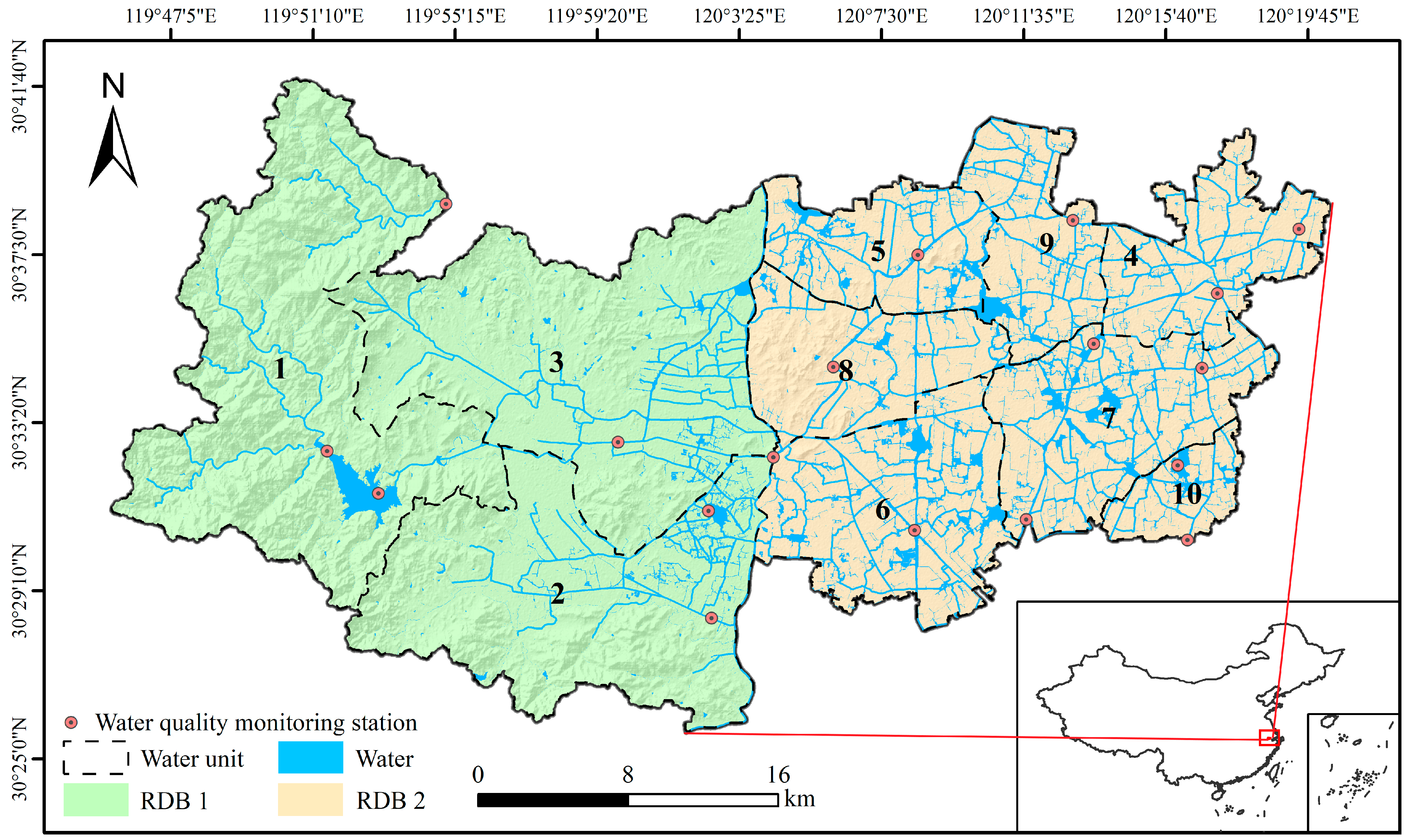
Figure 1. Distribution and spatial division map of water quality-monitoring stations in Deqing County.
Water 16 01319 g001
Figure 2. Landsat 8 data preprocessing process.
Water 16 01319 g002
Figure 3. Technology roadmap.
Water 16 01319 g003
Figure 4. Schematic diagram of remote sensing water quality sample data expansion method under the condition of air–ground spatiotemporal asynchrony.
Water 16 01319 g004
Figure 5. Expanded standards.
Water 16 01319 g005
Figure 6. Pixel-based SDG 6.3.2 evaluation method process.
Water 16 01319 g006
Figure 7. Water quality parameters and band correlation coefficient.
Water 16 01319 g007
Figure 8. RF feature importance and ReliefF feature parameter weight ranking of each solution (the left vertical axis is the feature weight, the right vertical axis is the cumulative proportion, and the horizontal axis is the selected feature variable).
Water 16 01319 g008
Figure 9. (a) Pearson correlation coefficient heat map of the 5-day raw dataset; (b) Pearson correlation coefficient heat map of the 8-day raw dataset.
Water 16 01319 g009
Figure 10. (a) The overall accuracy heat map of each solution model; (b) The Kappa coefficient heat map of each solution model.
Water 16 01319 g010
Figure 11. The number and proportion of high-quality water body pixels from 2013 to 2022.
Water 16 01319 g011
Figure 12. (a) Distribution frequency of poor water pixels from 2013 to 2017; (b) Distribution frequency of poor water pixels from 2018 to 2022.
Water 16 01319 g012
Figure 13. Distribution of poor water pixels in 2013, 2014, and 2015.
Water 16 01319 g013
Figure 14. (a) RDB1 SDG 6.3.2 evaluation result; (b) RDB2 SDG 6.3.2 evaluation result; (c) Deqing SDG 6.3.2 evaluation result.
Water 16 01319 g014
Figure 15. SDG 6.3.2 evaluation results at the water body unit scale in Deqing County from 2013 to 2022.
Water 16 01319 g015
Table 1. Classification feature set.
FeatureCalculation FormulaAmount
Single bandBi8
Band differenceBi − Bj28
Band ratioBi/Bj28
Normalized band ratio(Bi − Bj)/(Bi + Bj)28
Table 2. Water quality sample enhancement results.
Extended Time Window Total Amount of DataGood Water Quality Data VolumePoor Water Quality Data Volume
The day660
±1-day time window11110
±2-day time window534013
±3-day time window675215
±4-day time window967125
±5-day time window1128626
±6-day time window1169026
±7-day time window14211032
±8-day time window14411034
Table 3. Feature parameter combination scheme.
Feature Optimization MethodSample Expansion PlanWhether to Optimize
Single band±5-day time windowYes
±8-day time windowNo
Pearson correlation coefficient±5-day time windowYes
±8-day time windowNo
Random forest±5-day time windowYes
±8-day time windowNo
ReliefF±5-day time windowYes
±8-day time windowNo
Table 4. Annual average of measured data at monitoring stations, 2013–2015.
DO
(mg/L)
CODMn
(mg/L)
CODCr
(mg/L)
NH3-N
(mg/L)
Petroleum
(mg/L)
Fluoride
(mg/L)
TP
(mg/L)
Sampling Times
Target value for good water>=5<=6<=20<=1<=0.5<=1<=0.2
20135.5804.40920.0731.1420.0440.4920.170114
20146.3914.36918.0761.0180.0430.4160.125114
20156.4643.96515.3680.5320.0410.4190.112112
Disclaimer/Publisher’s Note: The statements, opinions and data contained in all publications are solely those of the individual author(s) and contributor(s) and not of MDPI and/or the editor(s). MDPI and/or the editor(s) disclaim responsibility for any injury to people or property resulting from any ideas, methods, instructions or products referred to in the content.