
Analysing Urban Flooding Risk with CMIP5 and CMIP6 Climate Projections

1
Centre for Applied Coastal Research, University of Delaware, Newark, DE 19717, USA
2
Institute of Urban and Industrial Water Management, TU Dresden, 01062 Dresden, Germany
*
Author to whom correspondence should be addressed.
Water 2024, 16(3), 474; https://doi.org/10.3390/w16030474
Submission received: 4 January 2024
/
Revised: 26 January 2024
/
Accepted: 27 January 2024
/
Published: 31 January 2024
(This article belongs to the Special Issue Innovative Flood Risk Management under Changing Environments)
Abstract
:Fitting probability distribution functions to observed data is the standard way to compute future design floods, but may not accurately reflect the projected future pattern of extreme events related to climate change. In applying the latest coupled model intercomparison project (CMIP5 and CMIP6), this research investigates how likely it is that precipitation changes in CMIP5 and CMIP6 will affect both the magnitude and frequency of flood analysis. GCM output from four modelling institutes in CMIP5, with representative pathway concentration (RCP8.5) and the corresponding CMIP6 shared socioeconomic pathways (SSP585), were selected for historical and future periods, before the project precipitation was statistically downscaled for selected cities by using delta, quantile mapping (QM), and empirical quantile mapping (EQM). On the basis of performance evaluation, a rainfall-runoff hydrological model was developed by using the stormwater management model (SWMM) for CMIPs (CMIP5 and CMIP6) in historical and future horizons. The results reveal an unprecedented increase in extreme events, for both CMIP5 (historical) and CMIP6 (future) projections. The years 2070–2080 were identified by both CMIP5 and CMIP6 as experiencing the most severe flooding.
Keywords:
probability distribution; climate change; CMIP5 and CMIP6; GCMs; RCPs; SSPs; delta; QM; EQM; hydrological model; flood risk analysis1. Introduction
Flooding is one of the most common natural disasters around the globe, and different regions of the world are experiencing catastrophic flood occurrences due to the increasing intensity and reoccurrence of heavy rainfall, resulting in severe loss of life and belongings [1]. An outbreak of flooding ravaged many European nations between 12–15 July 2021, claiming 243 lives, with Germany and Belgium accounting for 80.1% and 17.75% of the casualties, respectively. The cost of the damage was estimated to total ten billion euros, and both power and transport suffered major interruptions [2]. The aftermath of the 2012 ‘Sandy’ flood of New York revealed “43 deaths… 6500 patients evacuated from hospitals and nursing homes…Nearly 90,000 buildings in the inundation zone… 1.1 million New York City children unable to attend school for a week… close to 2 million people without power… 11 million travellers affected daily… $19 billion in damage” [3]. The aftermath of floods has a severe impact on humans, infrastructure, economics, and the environment, and the importance of effective risk management cannot be overemphasized. In order to achieve a resilient community, decision-makers must prioritize holistic and effective risk management techniques.
The traditional method for calculating future design floods is to fit probability distribution functions to records, which may not properly represent the likely future pattern of catastrophic occurrences resulting from climate change [4]. The generalized extreme value (GEV) and the generalized Pareto are the two primary statistical methods used in extreme event analysis [5,6]. The formulation of GEV and Gumbel distribution are similar, with the exception of extra shape parameters in the former. “Flood hazard” is the likelihood of flood occurrence and intensity, namely the water depth, discharge, and duration of inundation due to a possible flood event in a given metropolitan region over a particular period. These excessive external loads are caused by extreme precipitation or storms, which result in pluvial or coastal flooding, respectively. “Exposure” denotes the extent to which humans, infrastructure, and socio-economic activities are vulnerable to urban flooding. Receptors are connected to flood sources through a pathway.
The superimposition of the inundation extent map with the residential building standards is among the methodologies that this researcher suggests for providing information about spatially exposed urban environments [7]. Future extreme precipitation is not well captured by only fitting the exceedance probability of a historical precipitation, as incorporating climate changes into the assessment of future extreme event patterns in China is critical for developing regional flood risk reduction strategies for future climatic scenarios.
Due to the rising intensity of precipitation and its consequences, urban floods are causing considerable public concern and holistic risk assessment is therefore essential for effective urban flood management. There is ample evidence that the joint effect of climate change and growing urbanization is the principal cause of increased rainfall runoff [8]. The increasing effect of climate change on regional hydrological characteristics and the flood hazard in future climate patterns have received immense attention, and require a paradigm shift, in which techniques of flood risk assessment shift from conventional techniques to the populations and assets who have been identified as being vulnerable to future flooding by the output of global circulation models.
The coupled model inter-comparison project (CMIP) was a repository of a climate model for generating projections that was established by the World Climate Research Program [9]. The CMIP5 has created over 39 models, with huge improvements on the original, and uses an updated set of emission storylines known as representative concentration pathways (RCP), which produce valuable climate information for decision-makers and the research community [10]. CMIP6 follows the progression and adaption feature trend of the earlier CMIP5 by using shared socioeconomic pathways (SSPs). The CMIP6 framework connects social stories to physical radiative forcing pathways (RCPs), making a more robust and enhanced process [11]. Several researchers have tried to analyse the CMIP data, with the aim of examining the hydrometeorology trend in multiple scenarios in China.
The findings conclude that extreme temperature and precipitation have been generally rising in this century, with these changes more visible in the CMIP6 simulation than the CMIP5 [4,9,12]. And [9] reveals that flood frequency rises were most frequent in Asia, low-lying Africa, and South America, and this future trend of flood change was also similar in CMIP5 and CMIP6 [13]. However, while studies have demonstrated that CMIP5 performs well in the historical data, the CMIP6 models generally have higher spatial and temporal resolution (compared to CMIP5), and are therefore more suitable for detailed studies. The CMIP6 models aim to better represent certain critical climate processes (e.g., the cloud), making them more accurate than CMIP5 counterparts. The underlying potential means it is necessary to undertake a systematic analysis of the advantages and disadvantages of each projection that considers flood risk management.
China’s growing metropolitan areas, flourishing economy, and increasing population have suffered considerable flood damage in recent years [14]. A good percentage of the country’s urban infrastructure, and especially megacities, is vulnerable to a flood of different return periods. The National Climate Centre of China reported that China is the country most severely impacted by floods, with nearly 66 percent of the land area, more than half of the population, and 67 percent of agricultural and manufacturing production values exposed to danger every year, resulting in massive economic losses [1,15]. For example, 1998 flooding of the Yangtze River caused 3704 causalities, and 2013 floods in China killed 775 people and left 374 people missing [16]. Between 2000 and 2008, 748 flood disasters happened in China, per the statistics from the China Committee for National Disaster Reduction (CNCDR), aftermath 6624 deaths. Furthermore, 0.78383 billion people were impacted, 3.6 million buildings were affected, more than 123.6 million acres of crops were lost, and an economic cost of about RMB 290 billion was spent.
The urban runoff management infrastructure tends to lag behind urban expansion, and the occurrence and volume of city storm floods have rapidly risen [17], with many studies concluding that the impact of urban floods on life and socio-economic status is worse than before [5,15,18,19,20,21]. Flood events in China have been investigated by using web-based information to explore spatial and temporal trends, and it has been reported that almost 59.9% of China’s cities have been affected by a storm flood event, triple the amount that the government projected in 2011 [17]. The magnitude of flood impacts grew in the previous three decades, as a result of various physical, socioeconomic, and hydro-mereology factors [19]. Although GCMs potentially have great potential to capture this trend, their output is typically, as a result of spatial scale, too coarse to capture this change in urban areas. The downscaling approach is therefore necessary to convert large-scale GCM outputs to tailored regional scales of interest [22] Regional climate models (RCMs) have also been frequently employed in the downscaling GCM forecasts of future climate change scenarios. Downscaling techniques are divided into statistical and dynamic downscaling, namely RCMs [23,24]. Dynamical downscaling involves either performing a high-resolution restricted area model with GCM data as boundary conditions or conducting a “time slice” experiment [25]. The computing load imposed by the increase in resolution limits the practical implementation of dynamical downscaling. Measured long-term time series are used in statistical downscaling to build statistical correlations that involve local values and large-scale averages of surface variables. The statistics used might be basic or complex, but the ultimate correlations are usually determined by using some type of regression analysis [25] Statistical downscaling methods typically have broader applications because of their low computation efficiency and comparatively good performance [22]. The choice of statistical bias correction techniques is important because it affects the overall accuracy of downscale data.
Recognizing how floods evolve in a changing environment will improve future flood risk management, thus helping the decision-maker and community to tackle the flood. In acknowledging the importance of addressing the above overarching issues, this study aims to:
- Explore the future urban flood risk in different climate scenarios by using GCM projections.
- Analyse the applicability of CMIP5 and CMIP6 to flood risk by using a cross-regional comparative study.
- Explore the applicability of multiple downscaling methods to coupling global-scale climatic data with urban-scale hydrological analysis.
A detailed explanation of the research will be discussed further, and provide an additional reference for flood risk management in a wider context of climate change.
2. Materials and Methods
2.1. Study Area
Location
Shanghai, Beijing, and Guangzhou are the three most populated cities in China, with a very high flood risk [26,27] So the research focuses on the urban area, which accounts for 1.54%, 1.73%, and 1.09% of the total population, respectively. China’s climate varies, with humid, semi-humid, semiarid, and arid climatic zones with different watershed sizes. The western and northern parts of China have dry weather, and the eastern section has a semi-humid and humid environment [28]. The East Asian summer monsoon has an impact on eastern China., while Southwest China is influenced by a mix of the East Asian summer monsoon and the Indian summer monsoon, while Northwest China remains untouched. Most of continental China is located within the East Asian monsoon climatic zone, and so monthly, yearly, and inter-annual changes in precipitation, P, and air temperature, T, are visible [16,28]. The distribution of atmospheric precipitation throughout China’s huge landmass is highly inconsistent across both space and time (Figure 1). The average annual P varies from the northwest to the southeast, ranging between 15 mm and over 2200 mm, and the annual daily mean T changes from north to south, ranging between 12 and 25 °C.
2.2. Data Preparation
The DEM was accessed through the USGS national map explorer (https://earthexplorer.usgs.gov/, accessed between 20 April–28 May 2022). Although the previous finding recommends greater resolution DEM for a more accurate model [1], limitations resulted in this research adopting a 30-m resolution DEM issued by the USGS earth explorer [29] Figure 2A depicts the study area DEM.
The land cover and land use data were gathered at the Environmental Systems Research Institute (ESRI) https://env1.arcgis.com/arcgis/rest/services/Sentinel2_10m_LandCover/ImageServer, accessed between 20 April–28 May 2022). The LULC has a resolution of 10 m with nine classifications of mapped surface that cut across the built area, vegetation, agriculture, and water. Figure 2B illustrates the LULC of the study area. Hydrological models are characterised by uncertainty, ranging from data acquisition and choice of model to parameterization, amongst others. The data collection of the different institute experiments who participated in the World Climate Research Programme was downloaded from https://www.wcrp-climate.org/, which was between 3 March–15 May 2022 to obtain CMIP5 (RCP8.5) and CMIP6 (SSP5) GCM projections for historical and future periods. Table 1 and Table 2 show the model specifications. To maintain consistency, similar models from the same institute were selected for investigation with CMIP 5 and CMIP 6, with the variation categories r1i1p1 and r1i1p1f1, respectively [30] This ensured accurate comparison and performance evaluation. The CMIP5 explores the earlier RCP 8.5 in various greenhouse gas emission scenarios, and CMIP6 uses updated SSPs that consider potential changes in the global ecosystem and socioeconomic pattern [13,30].
The SM2RAIN–ASCAT (Soil Moisture to Rain—Advanced SCATterometer) rainfall data record covers the years 2007–2020, with a spatiotemporal resolution of 12.5 km/d. The Global historical precipitation was downloaded from Link: https://zenodo.org/records/6136294 (accessed between 3 March–15 May 2022). The new SM2RAIN–ASCAT data record was created by applying the SM2RAIN algorithm to the ASCAT soil moisture data records [31], the first instance when the SM2RAIN-ASCAT dataset matched the ASCAT soil moisture spatial resolution output.
2.3. Statistical Downscales
GCM results are typically too coarse to capture climatic variations at the watershed scale, and so a downscaling approach is necessary to convert large-scale GCM outputs to tailored regional scales of interest [22]. There are several statistical downscaling strategies and, of these, Bias Correction (BC) was one of the most successful and widely used to assess climate change impacts across the world [24]. To correct the deviation in GCM output, three common BC techniques were used [32].
2.3.1. The Delta Changes Technique
This technique, which is also referred to as “the perturbation method,” is a typical strategy used to minimize model uncertainties in climate change impact studies [33,34]. The approach develops climatic scenarios by combining daily or monthly data with the climate change signal (CCS) from GCM. CCS removes model lapses if they seem to be comparable in both timeframes, and also removes any plausible variation in temporal scale, as variability is derived from data. When the deltas change is calculated, the result can be applied to past climate data with a finer spatial resolution to provide projected climate forecasts for catchments of interest
where ∂ = Change factor or climate change signal, = future precipitation GCM simulated precipitation, = current precipitation GCM simulated precipitation, Pc = the currently observed regional-scale temperature.
2.3.2. The Empirical Quantile Mapping (EQM)
The techniques can be extensively applied to many GCM variables [33,35,36], and primarily involve generating the daily empirical cumulative distribution functions (ecdfs) on a point-by-point basis [33,35,36], which distinguishes it from other techniques adopted for precipitation by evaluating ecdfs for the wet and dry days separately. The EQM techniques concurrently adjust the recurrence of precipitation events and standard deviations. The downscale precipitation was computed by using Equation (2). The statistical distribution of model-simulated parameters is targeted to replicate the counterpart of observed parameters. A correction is then made by adapting the model data’s quantiles (percentiles) to the equivalents in the observed data.
where, PDS,m,d = Downscale precipitation, ecdfGCM,m = the empirical cumulative distribution functions of GCM in monthly, PGCM,m,d = monthly or daily precipitation from GCM.
2.3.3. Quantile Mapping
QM approaches use statistical transformations to resample the results of climate models. The statistical transformations entail using a mathematical relation to adapt the distribution functions of the predicted parameters into the recorded data, which may be represented formally as [33,35,36]. In correcting distortions in the mean and variance while maintaining the baseline model output’s spatial patterns and variability, quantile mapping offers several benefits. It is however important to acknowledge that quantile mapping is not an appropriate method for extremely rare events or complex interactions between variables, as it fails to consider variations in distribution form.
xo = observed parameter, f() = transformation function, xm = modelled parameter.
The quantile-quantile interaction was used to fuse the predicted variable distribution function to the measured counterpart. It is worth noting that the quantile connection of both measured and simulated variable data sets can be ascertained by using the CDFs, as shown [32]
cumulative distribution function of , = inverse form of the , CDF of = the quantile function.
2.4. Bias Correction Performance and Evaluation
The capacity of GCMs to simulate historical climate is determined by several factors, including the modelling trend, model network accuracy, and scientific awareness of specific physical processes [37]. Many previous studies used the bias indices to evaluate climate models by predicting hydrometeorological data, including the Taylor diagram [30,37,38,39,40,41]. Normalized root means square error (NRMSE) [30,40,41] Nash–Sutcliffe efficiency (NSE) [41,42].
2.4.1. Taylor Diagram
Sequence correlations, centralized pattern root-mean-square errors, and ratios of the standard deviations (RSD) of model results and data collected are used to create a Taylor diagram, which is a useful and concise way to study model competencies [38,39,40]. The means are removed before their second-order statistics are determined; the graphic does not give additional information about biases but only defines the centre pattern error [32]. These diagrams are useful for examining several features of complicated models or assessing the relative competence of numerous GCMs. Taylor’s skill score was computed by using Equation (5) [38].
The subscripts d and o are denoted and observed model, respectively. is the standard deviation Taylor scale (TS), which approximates to one if R and approaches R0 and respectively. And approach 0 indicates good performance.
2.4.2. Nash–Sutcliffe Efficiency (NSE)
2.4.3. The Normalized Root Means Square Error (NRMSE)
The NRMSE quantifies the discrepancy in both observed and simulated values and is often used in model performance evaluation [40]. The RMSE scale ranges from 0 to 1, with values closer to 0 indicating greater accuracy. The NRMSE in % is determined by using the formula.
2.5. Hydrological Model
The storm water management model (SWMM) has been widely used to study the rainfall runoff of a catchment around the world, including in Europe, North America [44] Asia [45,46,47] and the Middle East [48]. In Beijing, SWMM has been used to study rainfall runoff, optimal management practices, low-impact development, and sponge cities, in addition to other things [7,46,49,50,51,52]. Although SWMM has the capabilities of both hydrological and hydraulic models, it is an open source model that requires little data for modelling purposes [47], and can also simulate catchment situations at different spatial-temporal scales. In order to obtain the aforementioned benefit, this research employed SWMM 5.1 in hydrological modelling, which has been established to be a stable version [47]. The dynamic flow routing technique was adopted because it caters for backwater, friction loss, pressured flow, channel storage and is capable of achieving more accurate results [48]. Flooding happens when water depth exceeds the allowable threshold at the node.
2.5.1. Modelling Parameters
Research published in Beijing was used to identify the watershed characteristic parameters, such as the manning coefficient, coefficient (pervious/impervious), runoff computation techniques, the routing model, the infiltration model and mathematical modeling related to SWMM. These data are summarized in Table 3.
2.5.2. Model Calibration and Validation
SWMM calibration and validation specified the predominant characteristics of each underlying component needed to be determined, so that the results could replicate the catchment’s natural behavior [41,49,50]. The calibration procedure required modifications of design parameters so projection findings could be enhanced [49]. On the basis of past study findings and the parameter summary presented in Table 3, variables deeply linked to the correlations and pattern of measured precipitation and the projected precipitation of CMIP5 and CMIP6 were considered. This research used the percentage impervious [50,53], and the manning coefficient [50,53,54] in the calibration, and these parameters were carefully modified throughout the model calibration stage [55,56,57,58,59,60,61]. The schematic diagram of each sub—catchment and corresponding area is presented in the Figure 3 and detail framework for the research is showed in the Figure 4.
3. Results
The research results are discussed in relation to three themes. Section One addresses the result of the statistical downscale obtained for GCM by CMIP5 and CMIP6, which establish a basis for performance evaluation using the Taylor diagram and other selected criteria, as described in the methodology. Section Two presents the result of the rainfall-runoff model under the history in the years 1954 to 2012, with reference to the GCM projection of CMIp5 and CMIP 6. The results of the future projection (2015–2100) of the representative concentration pathway (RCP 8.5) by CMIP 5, and of the shared socio-economy pathway (SSP850) by CMIP 6, are also discussed. The final section presents analyses of the changed projection of CMIP5 and CMIP6, both in historical and future projections. Critical conclusions related to the changed magnitude and intensity of floods are also offered.
3.1. The Statistical Downscale
The result of the statistical downscale of the three Chinese cities (Beijing, Shanghai, and Guangzhou) is presented in this section in Figure 5, which presents a boxplot bias that cuts across them. Beijing shows a strong alignment between the downscaled and observed data, in the upper, middle, and lower quantiles. The whisker is also the result of all divergence under 5 mm/day of precipitation. In Guangzhou, the result indicates a bias in the observed and downscale data, whose variation ranges from 1–16 mm/day of rainfall. The positive quantile has the highest precipitation variation of up to 10 mm/ day. The deviation was however relatively small in the lower quantile, at around 1 mm/day of precipitation. The difference in the middle quantile was found to be lower when compared to the upper quantile, and lower when compared to the lower quantile. Downscale precipitation for Shanghai is high when compared to Beijing, and low when compared to Guangzhou. While there is no signification variation in the lower quantile, the upper quantile has a deviation of up to 7 mm/day of rainfall.
3.2. The Statistical Downscale Performance and Evaluation
The result of the performance evaluation of the statistical downscale is presented in this section. Evaluation criteria were grouped into two sections. Section One consists of seven indicators (RMSE, NRMSE, Pearson, Spearman, MAE, MBE, and NSE), and only the result of Beijing is presented; Guangzhou and Shanghai, in contrast, are presented in the appendix. Similarly, the Taylor diagram for Beijing is discussed, and the other two cities are presented in the appendix. Figure 6 depicts the result of the delta, QM, and EQM bias correction techniques, and their performance evaluation index for the selected CMIP5 and CMIP6 GCM models. The result from ACCESS1-3 (Figure 6 subplot 1 & 2), and a closer look at the delta method of downscale, indicates an improvement in CMIP6, compared to CMIP5. The RMSE, NRMSE, MAE, MBE and NSE change from 1.58, 1.32, 0.96, 0.01, and 0.221 in CMIP 5, respectively; and from 1.35, 1.07, 0.79, 0, and 0.307 in CMIP6, again respectively. In the QM, a similar observation was made about the downscale.
However, the mean bias error changed from 0.225 in CMIP5 to −0.02 in CMIP6, which implied that the QM method of downscaling underestimated the precipitation. The EQM also had results close to the QM, with the exception of slightly better performance in the mean bias of 0.19 (in CMIP5) and 0.10 (in CMIP6). The result of downscaled MPI GCM output with different bias correction methods is presented in Figure 6 (subplot three and four) for CMIP5 and CMIP6, respectively. In both CMIP5 and CMIP6 projection, there is a strong correlation between six of the seven evaluation criteria. However, a disparity was noticed in the MBE value changes in Delta, EQM, and QM, which were 0, −48, −0.64 to 0.01, −0.3, and −0.45, in CMIP5 and CMIP projection, respectively. No significant improvement was observed in the latest and earlier CMIP projection.
Figure 6 (subplots 5 & 6) depicts the downscaled result of CanESM GCM output by using three downscale statistical approaches. Nearly 86% of the evaluation criteria in CMIP5 and CMIP6 projection had similarities, with the exception of the MBE, and value change in EQM and QM, which went from −0.2 and −0.33 to 0.08 and 0.15 in CMIP5 and CMIP projection, respectively. Interestingly, the values were indifferent to delta techniques. No significant improvement was observed in the latest and earlier CMIP projection.
Figure 7 shows the Taylor diagram for Beijing city in CMIP5 and CMIP6 projection for the selected GCM models (ACCESS, BCC, CanESM, and MPI), along with corresponding statistical downscale results for the Delta, EQM, and QM, which were analysed. The downscaled CMIP5 ACCESS1-3 using EQM techniques recorded results close to the observed data, with RMSD values of 6.8, a correlation value of 0.67, and an SD value of 6.5. The models whose performance most closely resembles CMIP5 ACCESS1-3 are the CMIP5 EQM MPI-ESM-HR, CMIP5-EQM CanESM2 and CMIP5-EQM BCC-CSM1, which each had RMSD, correlation, and SD of 7.5, 0.64, and 8; 7.5, 0.64, and 8; and 7.8 0.58, and 8.5. But the downscaled MPI model using the QM downscale techniques recorded the maximum RMSD, correlation, and SD, of 13, 0.4, and 12.7.
Similar to the result of CMIP6, which showed a quite striking improvement in GCM output, the CanESM2—QM, ACCESS—EQM, CanESM2–EQM, BCC-CSM1—EQM, CanESM2—Delta, BCC-CSM1—QM, ACCESS1-3—Delta, and BCC-CSM1—Delta all recorded correlates greater than 0.60. The CanESM2—QM has a minimum RMSD deviation of 2 in the observed data, while MPI-ESM-HR QM has a maximum RMSD value of 15.
Outlet Comparison
The result of the hydrological modelling of rainfall-runoff in the measured data was obtained by a simulated case based on historical and future projection of CMIP5 and CMIP6 scenarios. On the basis of the outcome of the performance evaluation, the CanEsm downscaled precipitation was selected for hydrological modelling that would use the Beijing study area. The historical period spans the years 1954 to 2014 and the future era spans 2015 to 2100, which are both considered with the Representative concentration pathway (RCP 8.5), by CMIP 5, and the shared socio-economy pathway (SSP850), by CMIP6. The result of hydrological model calibration is presented in Figure 8.
The result of the hydrological m analysis of future projected scenarios between 1954 to 2015 in the CMIP5, CMIP6, and observed data are presented in Figure 9. The CMIP5 projection overestimated precipitation, while the CMIP projection was close to the measured data.
The result of the statistical analysis of future projected scenarios between 2015 to 2100 in the CMIP5 and CMIP6 are presented in Figure 10A,B, for CMIP5 and CMIP6, respectively. The low runoff event is filtered from the timeseries.
4. Discussion
The downscaled CMIP6 projection captured the temporal variation in precipitation, showing that when compared to the CMIP5, it is consistent with [4,9,12]. The improved performance of CMIP6 was due to a finer spatial resolution of the GCM models and improved representation of the complex earth process [9]. The CMIP5 runoff time-series result indicates a 4.8% decrement, as compared to the maximum runoff in an observed historical period. The runoff was dominated by an antecedent situation, with a higher flood frequency. However, the frequency was more often provoked, which agrees with [11]. This might pose a threat to the recovery and, most likely, result in an overwhelmed system. In the CMIP6, the result reveals a maximum flooding of 7675.898 m3/s in the year 2075, corresponding to 21,800 iterations. CMIP6 projects more severe flooding with a 56.9% increase when compared to CMIP5, along with a 49.33% increase when compared to observed historical floods. It was also dominated by high-intensity floods with a higher frequency.
A threshold of 1000 m3/s was introduced to exclude events with low runoff event from the base case (the measured data), and to simulate cases for the historical and future projection based on CMIP5 and CMIP6 scenarios [62]. Events above this threshold were classified as extreme events. The extreme event was further analyzed based on the percentage composition that exceeded certain thresholds in the historical period of 1954 to 2014, for both CMIP 5 and CMIP6. The event was dominated by flooding of 2000 m3/s. A total of 25% of the events fall under 1200 m3/s; another 25% of the events fall under 1400 m3/s; and 32.5% of the events are in the range of 1400 m3/s and 2000 m3/s. Events with 2800, 3000, 3200, 3400, 4600, and 5200 m3/s each constituted 1% of the catastrophe events.
A total of 186 events were identified, with a range between 1000.929 and 5833.825. Most of the events were characterized by 1800 m3/s, although an event with a magnitude of 5833.8 m3/s emerged from an observed historical case. A total of 38% of events are due to flooding less than 1400 m3/s, while nearly 41 of the 186 events were due to runoff in the range of 1400–1800 m3/s. In contrast, the CMIP6 event has a total of 86 events, which is, when compared to the CMIP5, quite close to the number of events in the observed case. Also, most events were dominated by a 1800 m3/s flood. Interestingly the percentage of events characterized by 3200 m3/s flood increased from 0% in both cases (to 4% in the CMIP6).
The CMIP5 projection revealed a high number of runoff events, and a total of 269 projected anticipated events. It is important to note that events with higher magnitude became more pronounced and reoccurred, accounting for 30.5% of the total event. This indicates a higher flood hazard in the future, which may be due to climate change.
The predicted CMIP 6 was very similar to CMIP5, although CMIP6 predicted a higher flood of magnitude. The sum of 254 severed floods was expected on the basis of the projection, and analysis of this event reveals an unprecedented range between 1000.271 and 7675.898 m3/s. This flood event was characterized by 44% of the cumulated events being above 2000 m3/s, and the remaining 55% was dominated by events below 2000 m3/s.
5. Conclusions
The research facilitates our understanding of the likely growth in the intensity and frequency of flood disasters induced by changes in climate, as projected by CMIP5 and CMIP5 in historical and future horizons. On the basis of the findings, the CMIP5 and CMIP6 models were found to be adequate in capturing precipitation changes in Beijing to a reasonable extent [53]. The study also reported that CMIP6 models significantly improved when compared to earlier CMIP5 versions. In addition, a study of CMIP6 models, when compared to CMIP5 models for seasonal variation, depicted a significant improvement in the seasonal pattern. The SWMM rainfall runoff for Beijing city unveiled an unprecedented increase in flooding, which posed a threat to the community. As a result, analysing future alterations allows us to examine the influence of both climatic and social change and recognize the broad shift in precipitation [63,64]. In the case of Beijing, the model result shows a reasonable degree of correlation between both the CMIP5 and CMIP6, which indicates the skill of GCM in capturing variation in precipitation, and is consistent with the findings of [37,38]. Similarly, the MAE, NRMSE, and RMSE demonstrate a good downscaled model performance. Conversely, NSE showed an unsatisfactory performance. Here it is important to note that the divergence of MBE was due to differences in bias correction techniques. In the historical era, the CMIP5 (rcp8.50) predicted the most severe runoff event when compared to the CMIP6 (SSP585) and, in the future horizon, the CMIP6 (SSP585) predicts maximum flood events when compared to the CMIP5 (rcp8.5). The years 2070–2080 were dominated by a peak flood event in future projection, by both CMIP5 (rcp8.50) and CMIP6(SSP585). The total number of 75 events in the observed historical year skyrocketed by the end of 2100 and, according to CMIP5 and CMIP6 projections, increased by 350% and 338%, respectively. Undoubtedly, the future will experience more severe and frequent floods. The study also illustrates differences in precipitation, the main driver of floods due to climate change, while CMIP5 predicts flood severity and re-occurrence.
6. Recommendations
The research focuses on assessing changes in precipitation patterns as a result of climate change, and does this by using GCM projections from CMIP5 and CMIP6. The downscale statistical method, utilizing Artificial Neural Network, Multiple Linear Regression, Genetic Programming, and a Wavelet–Neural Network hybrid model, was employed to enhance precipitation resolution at the catchment level. Four GCM institute outputs were analyzed, and it was suggested future studies should include more institutes and ensemble models to reduce bias. CMIP6 simulation results pending completion by 2023 will however warrant a reevaluation of the study when they become available. The analysis considered the rcp8.5 and SSp585 scenarios for CMIP5 and CMIP6 projections, respectively. The recommendation for future investigations include exploring scenarios like SSP1-2.6, SSP2-4.5, and SSP3-7.0 to project precipitation alterations for different emissions pathways. The hydrological model focused on rainfall-runoff modeling, suggested that best management practices (BMP), low impact development (LID), and possibly sponge city concepts should be incorporated into future research. The study utilized SWMM, which has a 1D modeling limitation that hinders GIS-based hazard, vulnerability, and risk mapping, and it was therefore suggested that future investigations should consider using modeling software such as HEC-Ras version 6.1 by US Army Corps of Engineers, USA Mike-Urban version 2023 by Danish Hydraulic institute Denmark, and InfoWorks version 23.2.6 by Autodesk, San Francisco, CA 94105, USA. In addition, the study advocates computing the cost implications of various flood risks with the aim of ensuring decision-makers are fully informed.
Author Contributions
R.O.: Data curation, software, writing; W.Y.: data acquisition, formal analysis, writing review and editing, mentorship. P.K.: supervision. All authors have read and agreed to the published version of the manuscript.
Funding
This research received no external funding.
Data Availability Statement
The original contributions presented in the study are included in the article, further inquiries can be directed to the corresponding author.
Acknowledgments
The authors would like to express their gratitude: 1. The SLUB Dresden for funding the article processing charges. 2. The European Union for funding the Erasmus joint master’s degree in flood risk management.
Conflicts of Interest
The authors declare no conflicts of interest.
References
- Pokhrel, I.; Kalra, A.; Rahaman, M.M.; Thakali, R. Forecasting of Future Flooding and Risk Assessment under CMIP6 Climate Projection in Neuse River, North Carolina. Forecasting 2020, 2, 323–345. [Google Scholar] [CrossRef]
- Fekete, A.; Sandholz, S. Here Comes the Flood, but Not Failure? Lessons to Learn after the Heavy Rain and Pluvial Floods in Germany 2021. Water 2021, 13, 3016. [Google Scholar] [CrossRef]
- PlaNYC In the Lower Manhattan Financial District Post-Sandy Credit: Alexius Tan. 2013.
- Bian, G.; Zhang, J.; Chen, J.; Song, M.; He, R.; Liu, C.; Liu, Y.; Bao, Z.; Lin, Q.; Wang, G. Projecting Hydrological Responses to Climate Change Using CMIP6 Climate Scenarios for the Upper Huai River Basin, China. Front. Environ. Sci. 2021, 9, 602. [Google Scholar] [CrossRef]
- Yin, J.; Yu, D.; Yin, Z.; Liu, M.; He, Q. Evaluating the Impact and Risk of Pluvial Flash Flood on Intra-Urban Road Network: A Case Study in the City Center of Shanghai, China. J. Hydrol. 2016, 537, 138–145. [Google Scholar] [CrossRef]
- Zhou, Q.; Mikkelsen, P.S.; Halsnæs, K.; Arnbjerg-Nielsen, K. Framework for Economic Pluvial Flood Risk Assessment Considering Climate Change Effects and Adaptation Benefits. J. Hydrol. 2012, 414–415, 539–549. [Google Scholar] [CrossRef]
- Yin, Z.; Yin, J.; Xu, S.; Wen, J. Community-Based Scenario Modelling and Disaster Risk Assessment of Urban Rainstorm Waterlogging. J. Geogr. Sci. 2011, 21, 274–284. [Google Scholar] [CrossRef]
- Emori, S.; Taylor, K.; Hewitson, B.; Zermoglio, F.; Juckes, M.; Lautenschlager, M.; Stockhause, M. CMIP5 Data Provided at the IPCC Data Distribution Centre; IPCC: Geneva, Switzerland, 2016. [Google Scholar]
- Hirabayashi, Y.; Tanoue, M.; Sasaki, O.; Zhou, X.; Yamazaki, D. Global Exposure to Flooding from the New CMIP6 Climate Model Projections. Sci. Rep. 2021, 11, 3740. [Google Scholar] [CrossRef] [PubMed]
- Chen, H.; Sun, J.; Lin, W.; Xu, H. Comparison of CMIP6 and CMIP5 Models in Simulating Climate Extremes. Sci. Bull. 2020, 65, 1415–1418. [Google Scholar] [CrossRef]
- Nauels, A.; Rogelj, J.; Schleussner, C.F.; Meinshausen, M.; Mengel, M. Linking Sea Level Rise and Socioeconomic Indicators under the Shared Socioeconomic Pathways. Environ. Res. Lett. 2017, 12, 114002. [Google Scholar] [CrossRef]
- Fan, X.; Miao, C.; Duan, Q.; Shen, C.; Wu, Y. The Performance of CMIP6 Versus CMIP5 in Simulating Temperature Extremes Over the Global Land Surface. J. Geophys. Res. Atmos. 2020, 125, e2020JD033031. [Google Scholar] [CrossRef]
- Xiang, Y.; Zhou, T.; Deng, S.; Shao, Z.; Liu, Y.; He, Q.; Chai, H. Nitrite Improved Nitrification Efficiency and Enriched Ammonia-Oxidizing Archaea and Bacteria in the Simultaneous Nitrification and Denitrification Process. Water Res. X 2023, 21, 100204. [Google Scholar] [CrossRef] [PubMed]
- Yang, W.; Yang, H.; Yang, D.; Hou, A. Causal Effects of Dams and Land Cover Changes on Flood Changes in Mainland China. Hydrol. Earth Syst. Sci. 2021, 25, 2705–2720. [Google Scholar] [CrossRef]
- Rubinato, M.; Nichols, A.; Peng, Y.; Zhang, J.M.; Lashford, C.; Cai, Y.P.; Lin, P.Z.; Tait, S. Urban and River Flooding: Comparison of Flood Risk Management Approaches in the UK and China and an Assessment of Future Knowledge Needs. Water Sci. Eng. 2019, 12, 274–283. [Google Scholar] [CrossRef]
- Sun, F.; Mejia, A.; Zeng, P.; Che, Y. Projecting Meteorological, Hydrological and Agricultural Droughts for the Yangtze River Basin. Sci. Total Environ. 2019, 696, 134076. [Google Scholar] [CrossRef]
- Jia, S.; Li, Y.; Lü, A.; Liu, W.; Zhu, W.; Yan, J.; Liang, Y.; Xiang, X.; Guan, Z. City Storm-Flood Events in China, 1984–2015. Int. J. Water Resour. Dev. 2019, 35, 605–618. [Google Scholar] [CrossRef]
- Abdellatif, M.; Atherton, W.; Alkhaddar, R.; Osman, Y. Flood Risk Assessment for Urban Water System in a Changing Climate Using Artificial Neural Network. Nat. Hazards 2015, 79, 1059–1077. [Google Scholar] [CrossRef]
- Budiyono, Y.; Aerts, J.C.J.H.; Tollenaar, D.; Ward, P.J. River Flood Risk in Jakarta under Scenarios of Future Change. Nat. Hazards Earth Syst. Sci. 2016, 16, 757–774. [Google Scholar] [CrossRef]
- Kundzewicz, Z.W.; Su, B.; Wang, Y.; Xia, J.; Huang, J.; Jiang, T. Flood Risk and Its Reduction in China. Adv. Water Resour. 2019, 130, 37–45. [Google Scholar] [CrossRef]
- Muis, S.; Güneralp, B.; Jongman, B.; Aerts, J.C.J.H.; Ward, P.J. Flood Risk and Adaptation Strategies under Climate Change and Urban Expansion: A Probabilistic Analysis Using Global Data. Sci. Total Environ. 2015, 538, 445–457. [Google Scholar] [CrossRef]
- Yang, L.; Wang, L.; Li, X.; Gao, J. On the Flood Peak Distributions over China. Hydrol. Earth Syst. Sci. 2019, 23, 5133–5149. [Google Scholar] [CrossRef]
- Dosio, A.; Jury, M.W.; Almazroui, M.; Ashfaq, M.; Diallo, I.; Engelbrecht, F.A.; Klutse, N.A.B.; Lennard, C.; Pinto, I.; Sylla, M.B.; et al. Projected Future Daily Characteristics of African Precipitation Based on Global (CMIP5, CMIP6) and Regional (CORDEX, CORDEX-CORE) Climate Models. Clim. Dyn. 2021, 57, 3135–3158. [Google Scholar] [CrossRef]
- Di Sante, F.; Coppola, E.; Giorgi, F. Projections of River Floods in Europe Using EURO-CORDEX, CMIP5 and CMIP6 Simulations. Int. J. Climatol. 2021, 41, 3203–3221. [Google Scholar] [CrossRef]
- Rummukainen, M. SwECL1M SWF.DIS H REGIONAL C LI MAT E MODELLING PROGRAMME SMHI Reports Meteorology and Climatology Methods for Statistical Downscaling of GCM Simulations. 1997. [Google Scholar]
- Yao, N.; Li, L.; Feng, P.; Feng, H.; Li Liu, D.; Liu, Y.; Jiang, K.; Hu, X.; Li, Y. Projections of Drought Characteristics in China Based on a Standardized Precipitation and Evapotranspiration Index and Multiple GCMs. Sci. Total Environ. 2020, 704, 135245. [Google Scholar] [CrossRef]
- Ding, Y.; Xu, J.; Wang, X.; Peng, X.; Cai, H. Spatial and Temporal Effects of Drought on Chinese Vegetation under Different Coverage Levels. Sci. Total Environ. 2020, 716, 137166. [Google Scholar] [CrossRef] [PubMed]
- Ayantobo, O.O.; Li, Y.; Song, S.; Yao, N. Spatial Comparability of Drought Characteristics and Related Return Periods in Mainland China over 1961–2013. J. Hydrol. 2017, 550, 549–567. [Google Scholar] [CrossRef]
- Kumar, Y.P.; Maheswaran, R.; Agarwal, A.; Sivakumar, B. Intercomparison of Downscaling Methods for Daily Precipitation with Emphasis on Wavelet-Based Hybrid Models. J. Hydrol. 2021, 599, 126373. [Google Scholar] [CrossRef]
- Hamed, M.M.; Nashwan, M.S.; Shahid, S.; Ismail, T.B.; Wang, X.J.; Dewan, A.; Asaduzzaman, M. Inconsistency in Historical Simulations and Future Projections of Temperature and Rainfall: A Comparison of CMIP5 and CMIP6 Models over Southeast Asia. Atmos. Res. 2022, 265, 105927. [Google Scholar] [CrossRef]
- Brocca, L.; Filippucci, P.; Hahn, S.; Ciabatta, L.; Massari, C.; Camici, S.; Schüller, L.; Bojkov, B.; Wagner, W. SM2RAIN-ASCAT (2007-2018): Global Daily Satellite Rainfall Data from ASCAT Soil Moisture Observations. Earth Syst. Sci. Data 2019, 11, 1583–1601. [Google Scholar] [CrossRef]
- Hamed, M.M.; Nashwan, M.S.; Shahid, S. Inter-Comparison of Historical Simulation and Future Projections of Rainfall and Temperature by CMIP5 and CMIP6 GCMs over Egypt. Int. J. Climatol. 2022, 42, 4316–4332. [Google Scholar] [CrossRef]
- Themeßl, M.J.; Gobiet, A.; Heinrich, G. Empirical-Statistical Downscaling and Error Correction of Regional Climate Models and Its Impact on the Climate Change Signal. Clim. Change 2012, 112, 449–468. [Google Scholar] [CrossRef]
- Sunyer, M.A.; Hundecha, Y.; Lawrence, D.; Madsen, H.; Willems, P.; Martinkova, M.; Vormoor, K.; Bürger, G.; Hanel, M.; Kriaučiuniene, J.; et al. Inter-Comparison of Statistical Downscaling Methods for Projection of Extreme Precipitation in Europe. Hydrol. Earth Syst. Sci. 2015, 19, 1827–1847. [Google Scholar] [CrossRef]
- Ahmed, K.; Shahid, S.; Nawaz, N.; Khan, N. Modeling Climate Change Impacts on Precipitation in Arid Regions of Pakistan: A Non-Local Model Output Statistics Downscaling Approach. Theor. Appl. Climatol. 2019, 137, 1347–1364. [Google Scholar] [CrossRef]
- Fauzi, F.; Kuswanto, H.; Atok, R.M. Bias Correction and Statistical Downscaling of Earth System Models Using Quantile Delta Mapping (QDM) and Bias Correction Constructed Analogues with Quantile Mapping Reordering (BCCAQ). J. Phys. Conf. Ser. 2020, 1538, 012050. [Google Scholar] [CrossRef]
- Zamani, Y.; Arman, S.; Monfared, H.; Azhdari Moghaddam, M.; Hamidianpour, M. A Comparison of CMIP6 and CMIP5 Projections for Precipitation to Observational Data: The Case of Northeastern Iran. Theor. Appl. Climatol. 2020, 142, 1613–1623. [Google Scholar] [CrossRef]
- Xu, H.; Chen, H.; Wang, H. Future Changes in Precipitation Extremes across China Based on CMIP6 Models. Int. J. Climatol. 2022, 42, 635–651. [Google Scholar] [CrossRef]
- Jiang, D.; Hu, D.; Tian, Z.; Lang, X.; Jiang, C.; Hu, D.; Tian, Z.P.; Lang, X.M. Differences between CMIP6 and CMIP5 Models in Simulating Climate over China and the East Asian Monsoon. Adv. Atmospheric Sci. 2020, 37, 1102–1118. [Google Scholar] [CrossRef]
- Chen, X.; Zhang, H.; Chen, W.; Huang, G. Urbanization and Climate Change Impacts on Future Flood Risk in the Pearl River Delta under Shared Socioeconomic Pathways. Sci. Total Environ. 2021, 762, 143144. [Google Scholar] [CrossRef]
- Gu, L.; Yin, J.; Zhang, H.; Wang, H.M.; Yang, G.; Wu, X. On Future Flood Magnitudes and Estimation Uncertainty across 151 Catchments in Mainland China. Int. J. Climatol. 2021, 41, E779–E800. [Google Scholar] [CrossRef]
- Song, Y.H.; Chung, E.S.; Shahid, S. Spatiotemporal Differences and Uncertainties in Projections of Precipitation and Temperature in South Korea from CMIP6 and CMIP5 General Circulation Models. Int. J. Climatol. 2021, 41, 5899–5919. [Google Scholar] [CrossRef]
- Zhang, Y.; Ren, Y.; Ren, G.; Wang, G. Precipitation Trends Over Mainland China From 1961–2016 After Removal of Measurement Biases. J. Geophys. Res. Atmos. 2020, 125, e2019JD031728. [Google Scholar] [CrossRef]
- El-Sharif, A.; Hansen, D. Application of Swmm to the Flooding Problem in Truro, Nova Scotia. Can. Water Resour. J. 2001, 26, 439–459. [Google Scholar] [CrossRef]
- Agarwal, S.; Kumar, S. Applicability of SWMM for Semi Urban Catchment Flood Modeling Using Extreme Rainfall Events. Int. J. Recent Technol. Eng. 2019, 8, 245–251. [Google Scholar] [CrossRef]
- Rai, P.K.; Chahar, B.R.; Dhanya, C.T. GIS-Based SWMM Model for Simulating the Catchment Response to Flood Events. Hydrol. Res. 2017, 48, 384–394. [Google Scholar] [CrossRef]
- Seenu, P.Z.; Venkata Rathnam, E.; Jayakumar, K.V. Visualisation of Urban Flood Inundation Using SWMM and 4D GIS. Spat. Inf. Res. 2020, 28, 459–467. [Google Scholar] [CrossRef]
- Nile, B.K.; Hassan, W.H.; Alshama, G.A. Analysis of the effect of climate change on rainfall intensity and expected flooding by using ann and swmm programs. ARPN J. Eng. Appl. Sci. 2019, 14, 974–984. [Google Scholar]
- Randall, D.A.; Wood, R.A.; Bony, S.; Colman, R.; Fichefet, T.; Fyfe, J.; Kattsov, V.; Pitman, A.; Shukla, J.; Srinivasan, J.; et al. Climate Models and Their Evaluation Coordinating. In Climate Change 2007: The Physical Science Basis. Contribution of Working Group I to the Fourth Assessment Report of the IPCC (FAR); Cambridge University Press: Cambridge, UK, 2007. [Google Scholar]
- Li, J.; Zhang, B.; Mu, C.; Chen, L. Simulation of the Hydrological and Environmental Effects of a Sponge City Based on MIKE FLOOD. Environ. Earth Sci. 2018, 77, 32. [Google Scholar] [CrossRef]
- Wijesekera, S. Using SWMM as a Tool for Floodplain Management in Ungauged Urban Watershed. Engineer 2012, 45, 1–8. [Google Scholar] [CrossRef]
- Bisht, D.S.; Chatterjee, C.; Kalakoti, S.; Upadhyay, P.; Sahoo, M.; Panda, A. Modeling Urban Floods and Drainage Using SWMM and MIKE URBAN: A Case Study. Nat. Hazards 2016, 84, 749–776. [Google Scholar] [CrossRef]
- Zhu, Y.Y.; Yang, S. Evaluation of CMIP6 for Historical Temperature and Precipitation over the Tibetan Plateau and Its Comparison with CMIP5. Adv. Clim. Change Res. 2020, 11, 239–251. [Google Scholar] [CrossRef]
- Ramteke, G.; Singh, R.; Chatterjee, C. Assessing Impacts of Conservation Measures on Watershed Hydrology Using MIKE SHE Model in the Face of Climate Change. Water Resour. Manag. 2020, 34, 4233–4252. [Google Scholar] [CrossRef]
- Wang, Y.; Zhang, Z.; Zhao, Z.; Sagris, T.; Wang, Y. Prediction of Future Urban Rainfall and Waterlogging Scenarios Based on CMIP6: A Case Study of Beijing Urban Area. Water 2023, 15, 2045. [Google Scholar] [CrossRef]
- Murphy, C.; Kettle, A.; Meresa, H.; Golian, S.; Bruen, M.; O’Loughlin, F.; Mellander, P.E. Climate Change Impacts on Irish River Flows: High Resolution Scenarios and Comparison with CORDEX and CMIP6 Ensembles. Water Resour. Manag. 2023, 37, 1841–1858. [Google Scholar] [CrossRef]
- Meresa, H.; Murphy, C.; Fealy, R.; Golian, S. Uncertainties and Their Interaction in Flood Hazard Assessment with Climate Change. Hydrol. Earth Syst. Sci. 2021, 25, 5237–5257. [Google Scholar] [CrossRef]
- Li, R.; Zhang, J.; Krebs, P. Global Trade Drives Transboundary Transfer of the Health Impacts of Polycyclic Aromatic Hydrocarbon Emissions. Commun. Earth Environ. 2022, 3, 170. [Google Scholar] [CrossRef]
- Li, P.; Zhang, J.; Krebs, P. Prediction of Flow Based on a CNN-LSTM Combined Deep Learning Approach. Water 2022, 14, 993. [Google Scholar] [CrossRef]
- Jiang, R.; Lu, H.; Yang, K.; Chen, D.; Zhou, J.; Yamazaki, D.; Pan, M.; Li, W.; Xu, N.; Yang, Y.; et al. Substantial Increase in Future Fluvial Flood Risk Projected in China’s Major Urban Agglomerations. Commun. Earth Environ. 2023, 4, 389. [Google Scholar] [CrossRef]
- Ding, X.; Liao, W.; Lei, X.; Wang, H.; Yang, J.; Wang, H. Assessment of the Impact of Climate Change on Urban Flooding: A Case Study of Beijing, China. J. Water Clim. Change 2022, 13, 2692–3715. [Google Scholar] [CrossRef]
- Meresa, H.; Tischbein, B.; Mekonnen, T. Climate Change Impact on Extreme Precipitation and Peak Flood Magnitude and Frequency: Observations from CMIP6 and Hydrological Models. Nat. Hazards 2022, 111, 2649–2679. [Google Scholar] [CrossRef]
- O’Neill, B.C.; Tebaldi, C.; Van Vuuren, D.P.; Eyring, V.; Friedlingstein, P.; Hurtt, G.; Knutti, R.; Kriegler, E.; Lamarque, J.F.; Lowe, J.; et al. The Scenario Model Intercomparison Project (ScenarioMIP) for CMIP6. Geosci. Model. Dev. 2016, 9, 3461–3482. [Google Scholar] [CrossRef]
- Taylor, K.E.; Stouffer, R.J.; Meehl, G.A. An Overview of CMIP5 and the Experiment Design. Bull. Am. Meteorol. Soc. 2012, 93, 485–498. [Google Scholar] [CrossRef]
Figure 1.
The spatial distribution of average precipitation and the temporal variability of annual precipitation (blue) and yearly river discharge (black) Subfigure (a–k) illustrate temporal variation in precipitation in different location across China precipitation (blue) and yearly river discharge (black) [20].
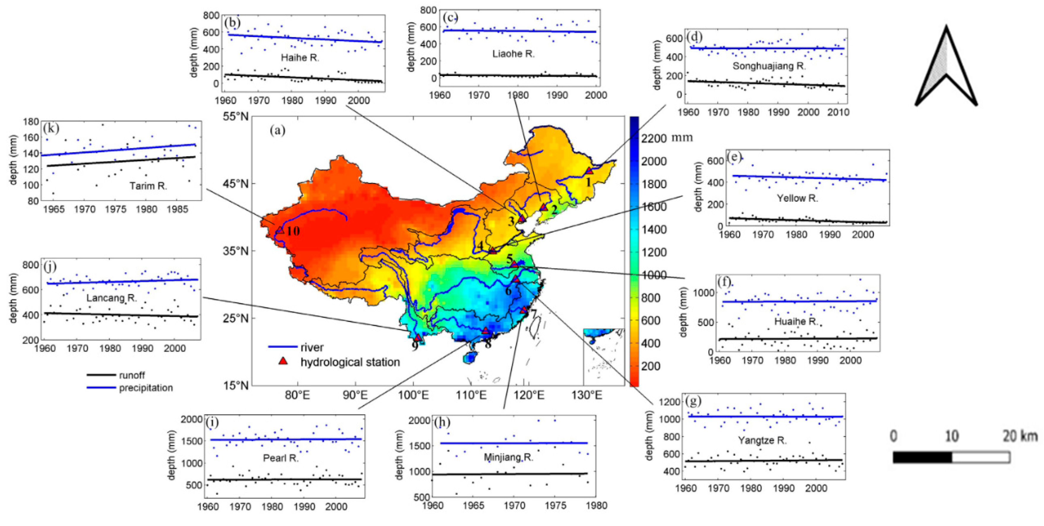
Figure 2.
(A) is the digital elevation model of Beijing, and (B) is 2021 landuse, which was captured by Living Atlas.
Figure 2.
(A) is the digital elevation model of Beijing, and (B) is 2021 landuse, which was captured by Living Atlas.
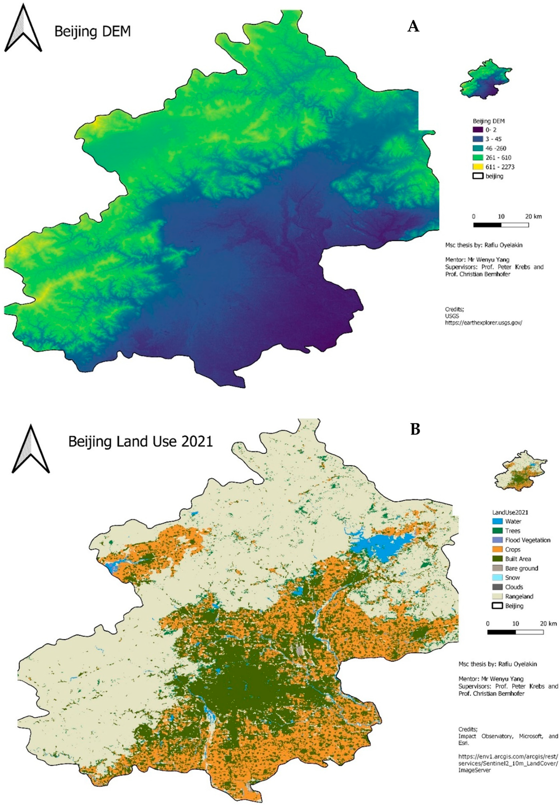
Figure 3.
Overview of the SWMM model and sub catchment area.
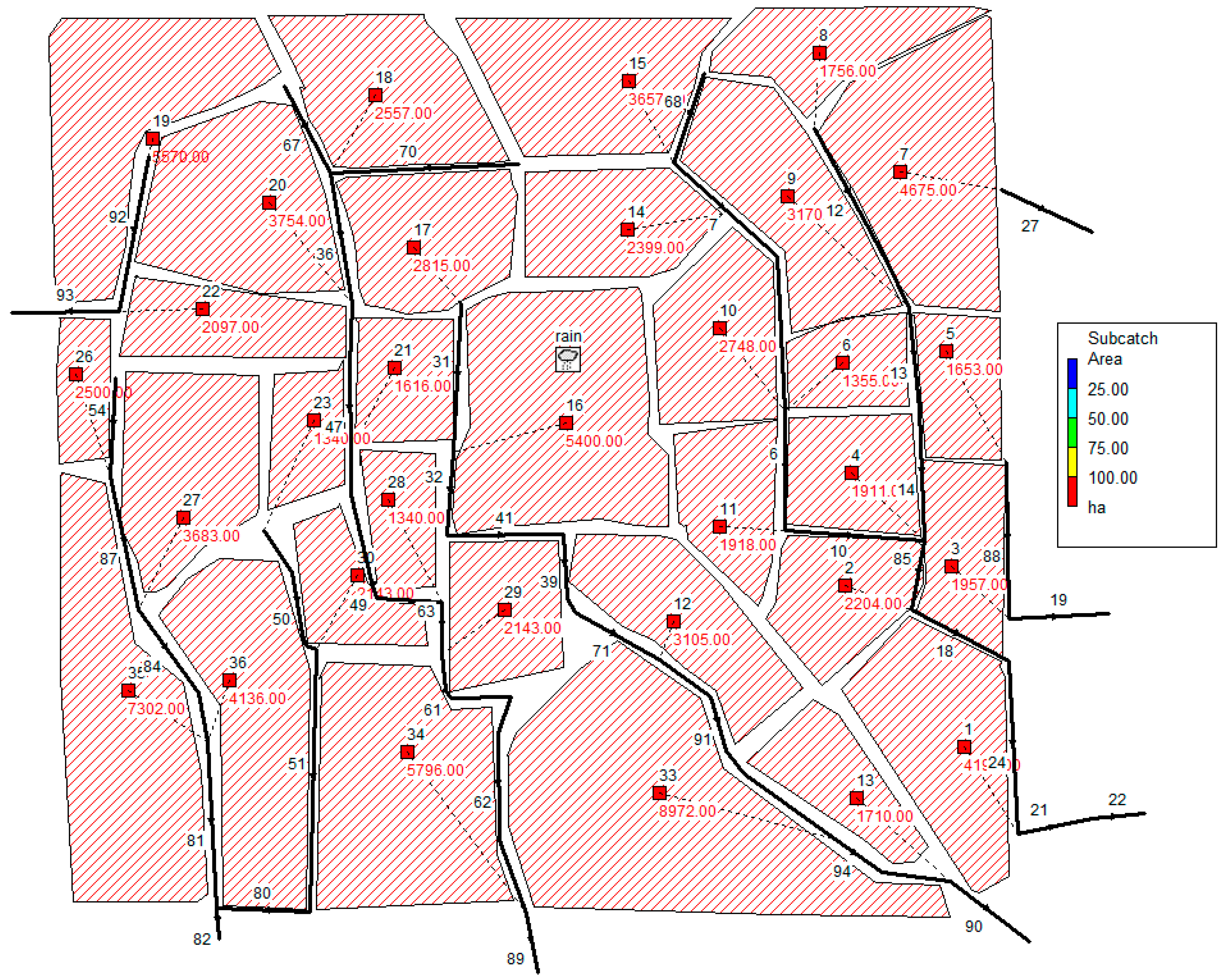
Figure 4.
Research methodology framework.
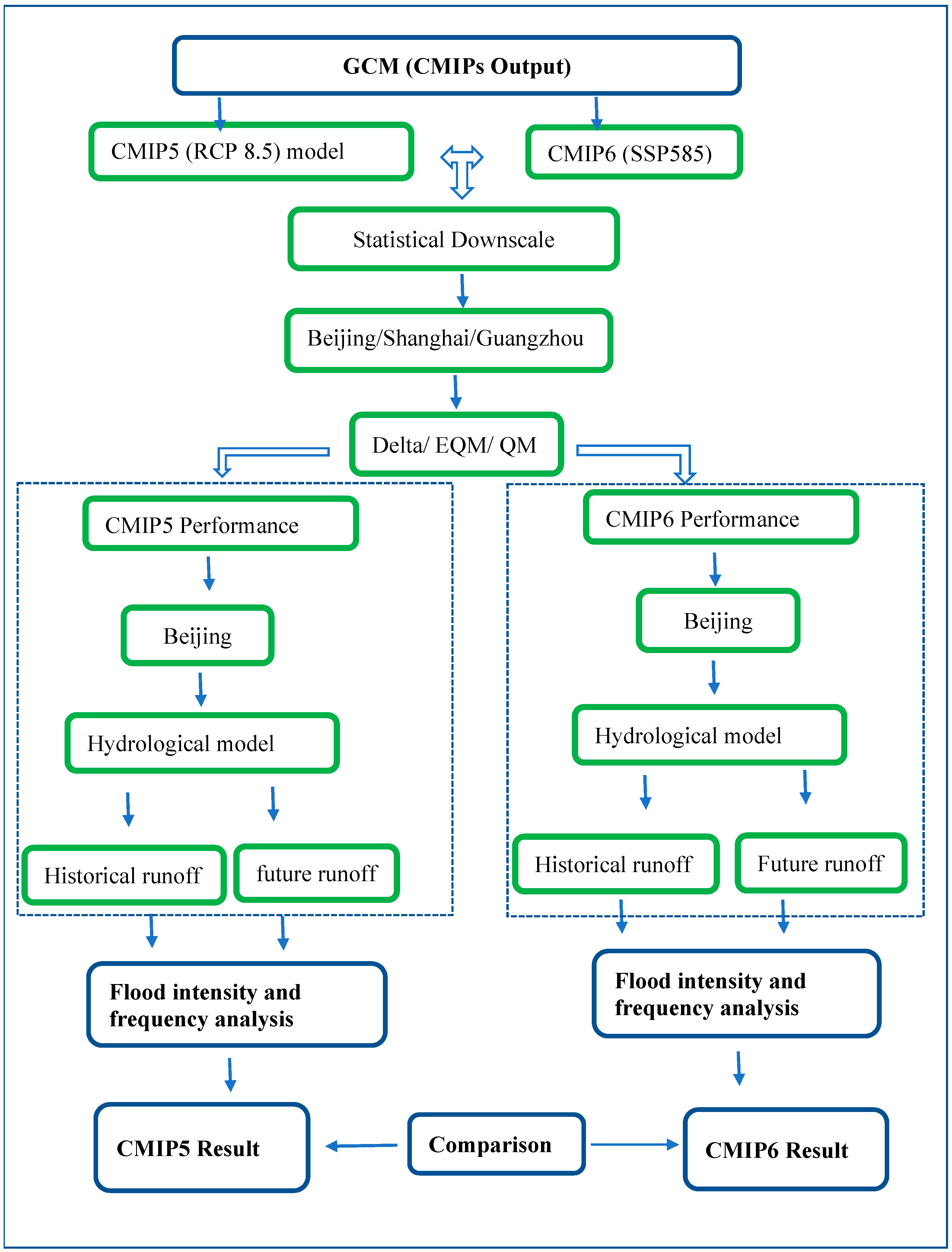
Figure 5.
Box plot for the downscaled bias for study cities.
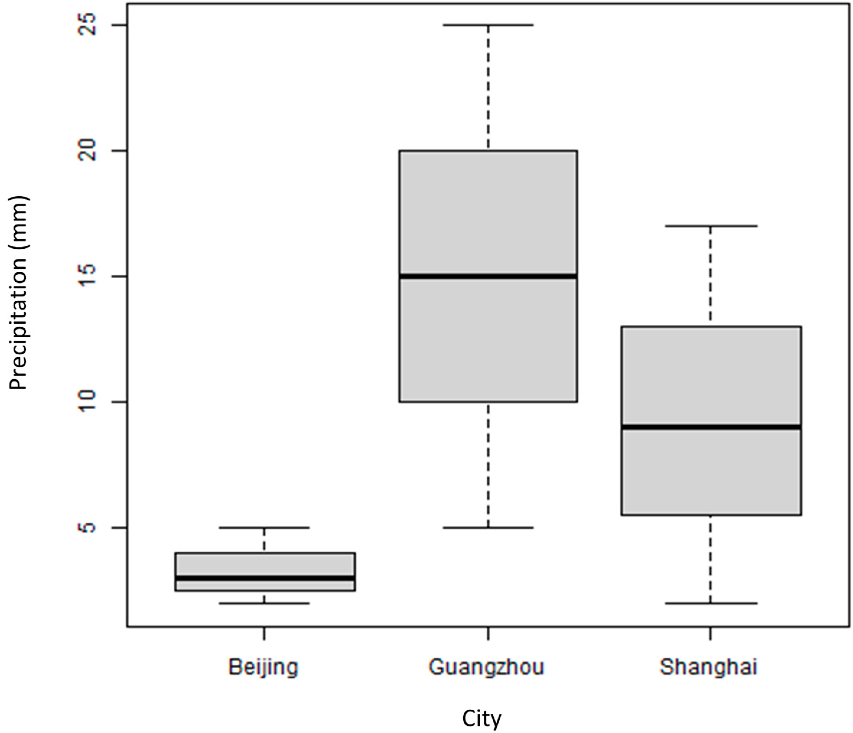
Figure 6.
Performance evaluation of the selected GCM model for Beijing City.
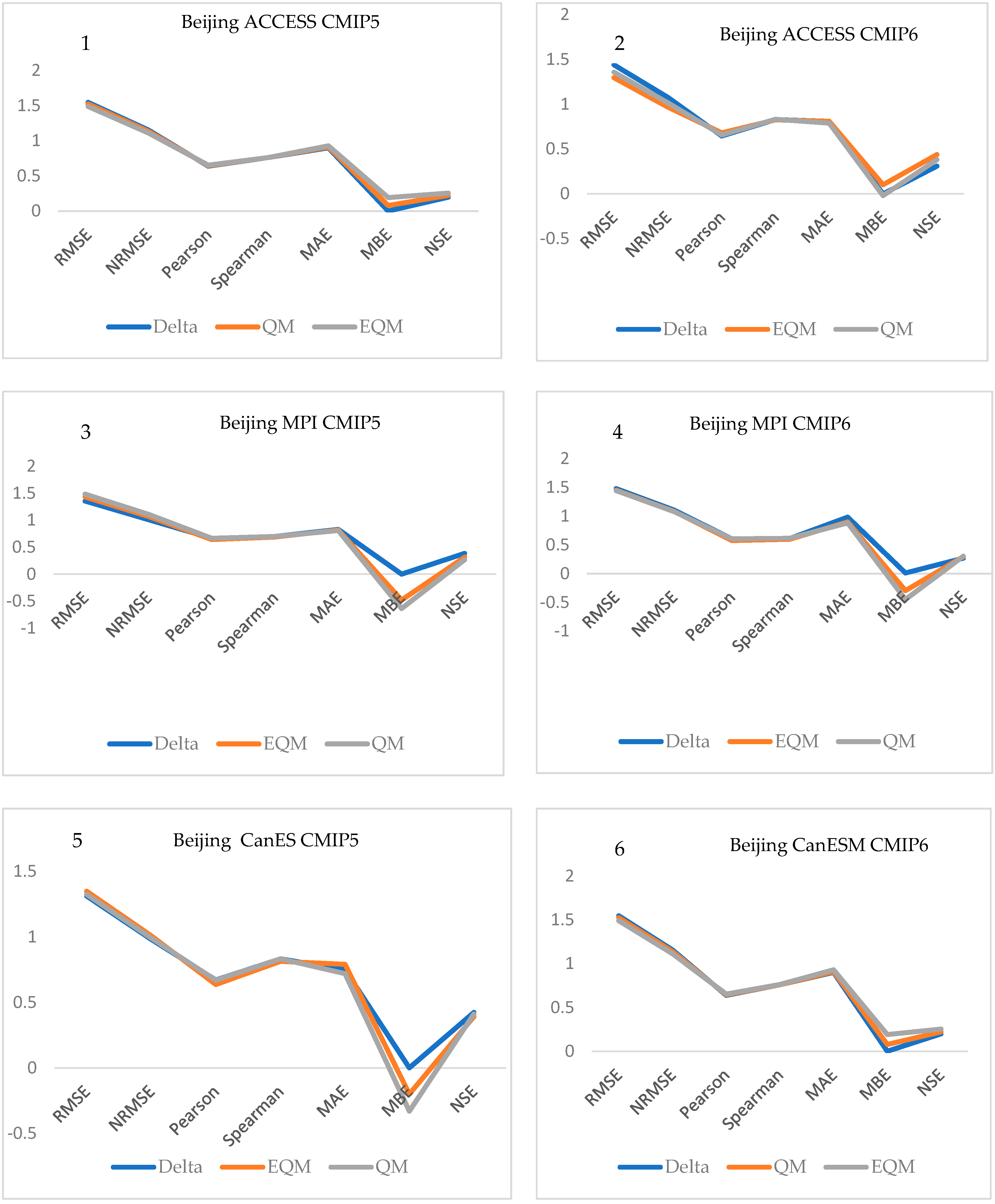
Figure 7.
Diagram from Beijing under CMIP5 and CMIP 6 projection.
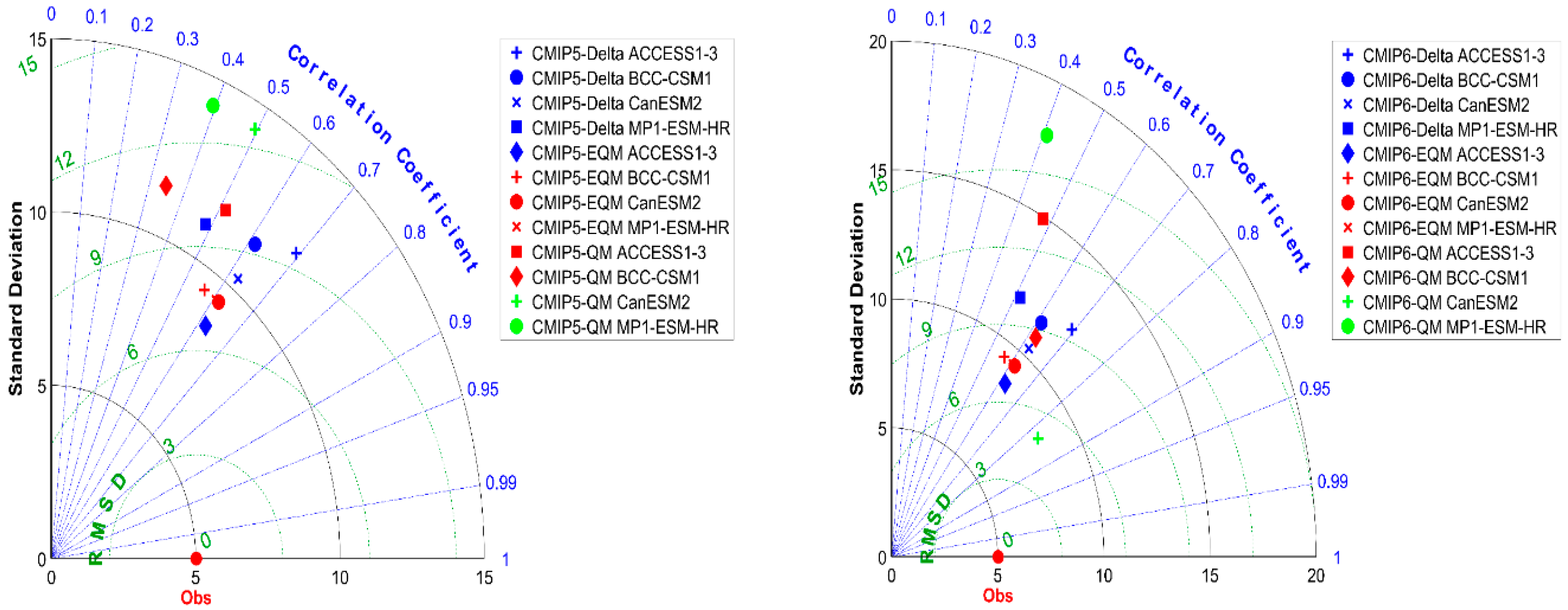
Figure 8.
Hydrological calibration at manning roughness n = 0.0109.
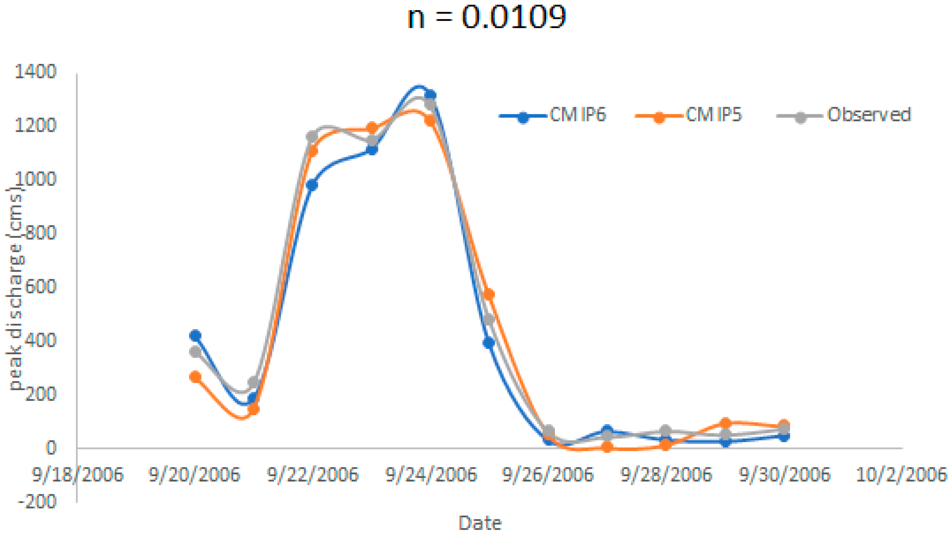
Figure 9.
(A): The runoff time series for Beijing in the simulated historical period, obtained by CMIP5, CMIP6 and observed data (between 1954–2014). (B): The runoff timeseries for Beijing in the simulated future period, obtained by CMIP5 and CMIP6 (between 2015 to 2100).
Figure 9.
(A): The runoff time series for Beijing in the simulated historical period, obtained by CMIP5, CMIP6 and observed data (between 1954–2014). (B): The runoff timeseries for Beijing in the simulated future period, obtained by CMIP5 and CMIP6 (between 2015 to 2100).


Figure 10.
(A): statistical analysis of runoff exceeding 1000 m3/s between 2015 and 2100 by CMIP5. (B): statistical analysis of runoff exceeding 1000 m3/s between 2015 and 2100 by CMIP6.
Figure 10.
(A): statistical analysis of runoff exceeding 1000 m3/s between 2015 and 2100 by CMIP5. (B): statistical analysis of runoff exceeding 1000 m3/s between 2015 and 2100 by CMIP6.


Table 1.
Model information for the selected CMIP 5.
| s/n | Model Name | Institute | Spatial Resolution | RCPs |
|---|---|---|---|---|
| 1 | bcc-csm1-1 | Beijing Climate Centre, China | RCP8.5 | |
| 2 | MPI-ESM-MR | Max Planck Institute for Meteorology, Germany | RCP8.5 | |
| 3 | CanESM | The Canadian Earth System Model | RCP8.5 | |
| 4 | ACCESS | Australian Community Climate and Earth System Simulator | RCP8.5 |
Table 2.
Model information for the selected CMIP 6.
| s/n | Model Name | Institute | Spatial Resolution | RCPs |
|---|---|---|---|---|
| 1 | BCC-CSM2-MR | Beijing Climate Center, China | 1.12 × 1.12° | SSP 5 |
| 2 | MPI-ESM1-2-HR | Max Planck Institute for Meteorology, Germany | 0.94 × 0.94° | SSP 5 |
| 3 | CESM2 | The Canadian Earth System Model | 1.00 × 1.25° | SSP 5 |
| 4 | ACCESS | Australian Community Climate and Earth System Simulator | 1.12 × 1.12° | SSP5 |
Table 3.
Summary of modelling parameters.
| Parameters | Parameters Description | Unit | Range |
|---|---|---|---|
| % Impervious | The ratio of impervious area | % | 12–100 |
| Area | Area of the sub-catchment | Hectares | 1340–8972 |
| Width | Width coefficient of the sub-catchment | m | 2.06–12 |
| Slope | Average percent slope of the sub-catchment | % | 0.3–2 |
| N-Impervious | Manning coefficient in impervious area | - | 0.011–0.15 |
| N-Pervious | Manning coefficient in pervious area | - | 0.05-0.8 |
| S-Impervious | Depression storage depth in impervious area | mm | 1.27–2.54 |
| S-Pervious | Depression storage depth in pervious area | mm | 2.54–7.62 |
| Manning | coefficient of the roughness of the conduit | - | 0.011–0.024 |
Disclaimer/Publisher’s Note: The statements, opinions and data contained in all publications are solely those of the individual author(s) and contributor(s) and not of MDPI and/or the editor(s). MDPI and/or the editor(s) disclaim responsibility for any injury to people or property resulting from any ideas, methods, instructions or products referred to in the content. |
© 2024 by the authors. Licensee MDPI, Basel, Switzerland. This article is an open access article distributed under the terms and conditions of the Creative Commons Attribution (CC BY) license (https://creativecommons.org/licenses/by/4.0/).
Share and Cite
MDPI and ACS Style
Oyelakin, R.; Yang, W.; Krebs, P. Analysing Urban Flooding Risk with CMIP5 and CMIP6 Climate Projections. Water 2024, 16, 474. https://doi.org/10.3390/w16030474
AMA Style
Oyelakin R, Yang W, Krebs P. Analysing Urban Flooding Risk with CMIP5 and CMIP6 Climate Projections. Water. 2024; 16(3):474. https://doi.org/10.3390/w16030474
Chicago/Turabian StyleOyelakin, Rafiu, Wenyu Yang, and Peter Krebs. 2024. "Analysing Urban Flooding Risk with CMIP5 and CMIP6 Climate Projections" Water 16, no. 3: 474. https://doi.org/10.3390/w16030474
Note that from the first issue of 2016, this journal uses article numbers instead of page numbers. See further details here.