
A Multi-Approach Analysis for Monitoring Wave Energy Driven by Coastal Extremes


1
Normandy University, UNICAEN, UNIROUEN, CNRS, UMR 6143 M2C, 14000 Caen, France
2
Normandy University, UNIROUEN, UNICAEN, CNRS, UMR 6143 M2C, 76000 Rouen, France
*
Author to whom correspondence should be addressed.
Water 2024, 16(8), 1145; https://doi.org/10.3390/w16081145
Submission received: 14 March 2024
/
Revised: 11 April 2024
/
Accepted: 16 April 2024
/
Published: 18 April 2024
(This article belongs to the Special Issue Hydrodynamics and Sediment Transport in the Coastal Zone)
Abstract
:This research investigates the behavior and frequency evolution of extreme waves in coastal areas through a combination of physical modeling, spectral analysis, and artificial intelligence (AI) techniques. Laboratory experiments were conducted in a wave flume, deploying various wave spectra, including JONSWAP (γ = 7), JONSWAP (γ = 3.3), and Pierson–Moskowitz, using the dispersive focusing technique, covering a broad range of wave amplitudes. Wave characteristics were monitored using fifty-one gauges at distances between 4 m and 14 m from the wave generator, employing power spectral density (PSD) analysis to investigate wave energy subtleties. A spectral approach of discrete wavelets identified frequency components. The energy of the dominant frequency components, d5 and d4, representing the peak frequency (fp = 0.75 Hz) and its first harmonic (2fp = 1.5 Hz), respectively, exhibited a significant decrease in energy, while others increased, revealing potential correlations with zones of higher energy dissipation. This study underscores the repeatable and precise nature of results, demonstrating the Multilayer Perceptron (MLP) machine learning algorithm’s accuracy in predicting the energy of frequency components. The finding emphasizes the importance of a multi-approach analysis for effectively monitoring energy in extreme coastal waves.
1. Introduction
Nowadays, chronic coastal hazards, including wave-driven flooding and erosion, are increasing in frequency and severity due to induced sea-level rise (SLR) and modified storminess patterns in the global context of climate change [1,2]. Their impacts are also influenced by internal system characteristics, such as geometry, topography slope, and sediment texture. These impacts are generally manifested through a series of changes, including coastal mechanisms and extensive economic and social costs [3,4]. Extreme waves are typically generated in open seas during energetic storms and exhibit a spatiotemporal spectrum in nearshore zones. Their frequencies are modulated in areas of reduced depths, such as surf zones. Therefore, characterizing nearshore wave behavior is key for reliable predictions of sediment transport, shoreline evolution, and future coastal management, including maritime structures and marine energy devices. The response of coastal zones to extreme events has been studied in previous works using observational methods, such as space and airborne techniques, numerical modeling, and laboratory experiments.
The physical characterization provided by the latter approach is essential in engineering solutions for coastal issues. Extensive research has been performed on wave characteristics in wave flumes [5]. Complicated physical processes, such as wave breaking, nonlinear wave–wave interactions, and energy transfer, are involved in the propagation of these extreme events in the form of steep wave trains [6,7].
At the laboratory scale, various methods exist for generating extreme waves, as discussed in [8,9,10]. Only the dispersive focusing mechanism for extreme wave generation [10,11,12,13,14] is considered in this paper. By combining several analytical techniques, the present study aims to gain insight into the relationships between wave behavior and energy dissipation.
In the literature, extreme waves are defined as large water waves with a crest-to-trough wave height H that exceeds twice the significant wave height Hs of the wave field [15,16]. The experimental results demonstrate a relationship between a water depth drop and an increase in the probability of extreme waves [17,18]. In ocean engineering, the wavelet analysis technique has been employed to explore the spectral components of non-stationary oceanographic drivers, such as waves and storm surges [19]. This method has been employed to discern wave groups with varying bathymetry [20], thereby predicting the occurrence of extreme events. While the Fourier transform analysis provides information about the frequency content of a signal over its entire duration, wavelet transforms offer time–frequency localization.
According to the existing literature, prior studies have often relied on short-duration signals, resulting in an insufficient consideration of the temporal aspects of extreme events. Additionally, a limited application of wavelet transforms in coastal studies has been noticed. In particular, the Maximal Overlap Discrete Wavelet Transform (MODWT) is well suited for detecting and analyzing intricate frequency components within coastal signals [21,22]. Despite its potential, this method has not been widely adopted in the current research methodologies. Furthermore, rapid advances in wave forecasting have made machine learning (ML) a valuable tool, providing a wealth of techniques for extracting information from data [23,24,25]. The Multilayer Perceptron (MLP) algorithm [26,27] was selected from several machine learning algorithms for its applicability to complex nonlinear problems and its ability to handle large input data sets [28]. This model has demonstrated its effectiveness [29] and will be employed to improve wave prediction based on experimental data.
The objectives of this work are delineated as follows: (1) Monitoring wave energy content using power spectral density analysis which provides a thorough comprehension of energy distribution across various frequencies in the wave spectrum. This allows the analysis of energy dissipation while varying the extreme events duration. (2) Identifying inherent frequency components and their assigned energy using the MODWT method. These aforementioned objectives will be fulfilled by the use of different approaches of physical modeling, spectral analysis, and artificial intelligence techniques. The coupling between different approaches will be useful to enhance our understanding of the energy behavior with its different frequency components.
This paper is organized into several sections. In Section 2, the experimental setup and the tested wave conditions are introduced. The monitoring of wave energy behavior extracted from the power spectral density and frequency component study are outlined in Section 3. Finally, Section 4 concludes with this paper’s findings, along with an overview of a learning algorithm application.
2. Materials and Methods
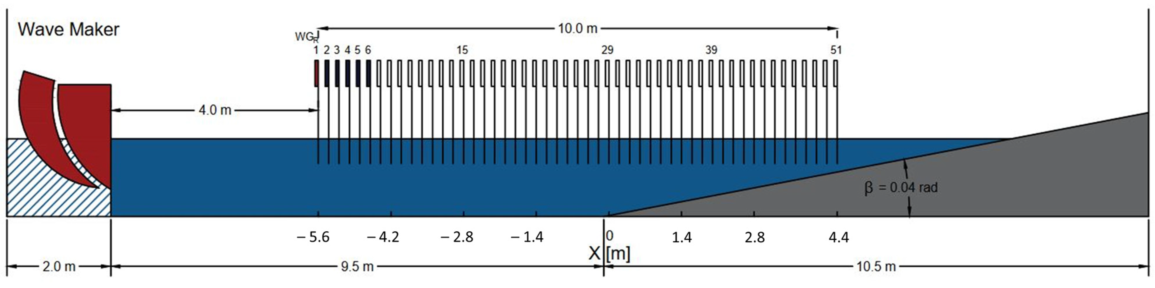
All experiments were performed at the wave flume in the Continental and Coastal Morphodynamics laboratory in Caen. This flume’s length is 20 m, the width is 0.8 m, and the useful height ranges from 25 cm to 40 cm (Figure 1). To simulate different wave conditions, a piston-type wave generator from Edinburgh Designs Ltd. (Edinburgh, UK) was used.
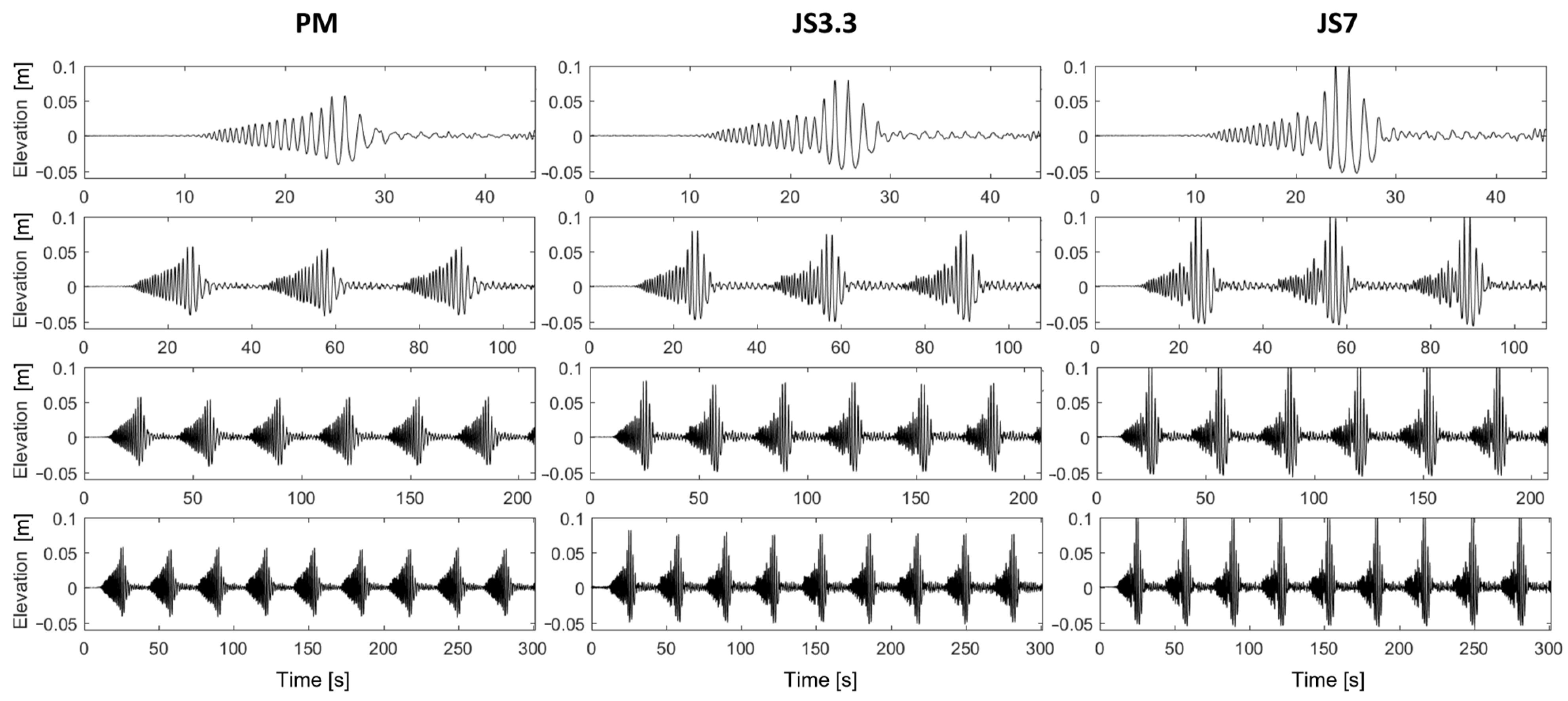
Three wave spectra were chosen, including JONSWAP (γ = 7), JONSWAP (γ = 3.3), and Pierson–Moskowitz, covering a wide range of amplitudes. The reference wave gauge (WGR) signals for the three spectra mentioned earlier, using various numbers of wave trains, are shown in Figure 2. To account for the varying duration of extreme events, one, three, six, and nine wave trains were generated (see Figure 2). Wave gauges positioned between 4 m and 14 m from the wave generator were used to measure the free surface elevation with a sampling rate of 32 Hz. Table 1 presents a summary of the parameters used.
The experimental configuration included two distinct sections: (1) A flat glass bottom, providing a hydraulically smooth surface; moreover, the water depth h0 within this section was set at 0.3 m. (2) An inclined PVC slope positioned at a distance of 9.5 m from the wave generator; the slope angle β was defined as 1/25 [30], corresponding to a slope gradient that enables wave transformation.
As shown in Figure 1, WGR refers to the reference wave gauge located 4 m away from the wave generator. To cover the 10 m experimental area, five wave gauges were strategically placed 20 cm apart [31]. This arrangement was replicated ten times. Wave breaking was imposed at 2 m from the slope’s toe.
The present focused wave groups use the linear NewWave profile [32,33] as their input. Each wave train consists of n sinusoidal wave components that phase together at a single point in time and space. The free surface elevation is expressed as follows using the linear wave theory (LWT):
where x represents the distance to the mean wave-maker position, t represents the time, ai is the wave amplitude of the ith component, ki is the wave number, ωi is the wave angular frequency, and ϕi is the phase angle at the focusing point.
The input parameters of Equation (1) are steepness, wave spectrum type, phase at focus, focus location, and peak frequency (fp). The focus of a wave train is mainly depending on dispersion (Equation (2)).
where ks represents the characteristic wavenumber and fs represents the characteristic frequency. Wave trains propagated in intermediate water depth are represented by [34], where denotes the wave number related to the wave peak frequency , and is the water depth. The initial local wave nonlinearity () of the wave train is determined from the free surface elevation obtained by the resistive probe placed 4 m from the wave-maker. We consider that the wave train is well formed by this point. The parameter was calculated using the formula (Equation (3)) (see [35]), as follows:
where is phase velocity, g is gravitational acceleration, and H is the maximum wave height at the focusing point (from the wave crest to the wave trough) calculated from the time series.
The wave trains generated are based on a Pierson–Moskowitz (Equation (4)) [36] or a JONSWAP (Equation (5)) spectrum [37]. The Pierson–Moskowitz spectrum can be described by the following equation:
where α = 0.0081: Philips constant determined empirically; fp = : peak frequency where = 0.14; and represents the wind speed on the fetch at 19.5 m of the free surface. A correction factor was added to the Pierson–Moskowitz spectrum, the peak enhancement factor γ, to improve the prediction of the energy spectral density of sea states. Therefore, the JONSWAP spectrum (Joint North Sea Wave Project) can be defined by the following equation:
where ; ; and if and 0.09 if .
The peak enhancement factor γ determines the height of the peak and the narrowness of the spectrum. For practical purposes, it usually ranges from 1 for a Pierson–Moskowitz spectrum to 7 for the narrowest spectrum.
3. Results and Discussion
3.1. Power Spectral Density
Spectral analysis provides the dissection of temporal signals into their component frequencies. This method is especially advantageous for comprehending fast time-varying phenomena like waves. It can be utilized to establish features such as dominant frequencies, harmonic content, periodicity, and quantify the energy dissipation during wave propagation (see [6,7,30]). The measured signals were low-pass-filtered to eliminate the spurious high-frequency band that could be contaminated by the electronic noise from the wave probes. The spectra were estimated using Welch’s method. A 50% overlap was employed to divide the signals into multiple segments. Each segment of the signal (approximately 16s) was first subjected to the Hann window before undergoing a 210-point fast Fourier transform (FFT), which produced a high spectral resolution of ∆f = 0.03125 Hz.
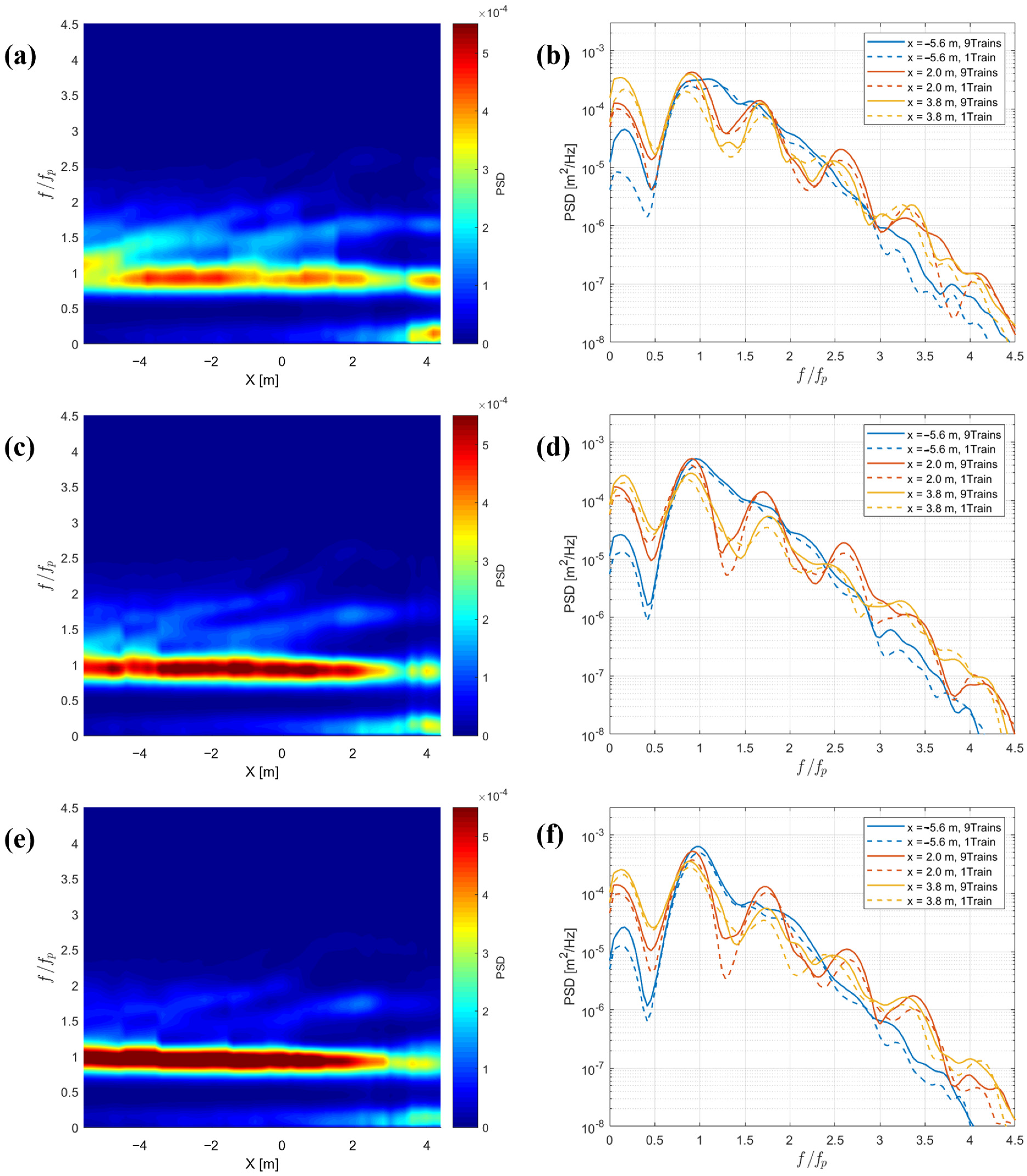
The spatial evolution of the spectrum as well as the detailed spectra at three specific positions are provided in Figure 3 and Figure 4 using the same nonlinearity . These positions were x = −5.6 m, x = 2 m, and x = 3.8 m, where 0 is the toe of the slope, corresponding to WG1 representing the initial wave signal , WG39 describing the signal before wave breaking , and finally WG48 as the last position , respectively. Two scenarios were examined, a single wave train signal (Figure 3) and a nine wave train signal (Figure 4).
Figure 3 shows that the spectrum of waves undergoes a widening process as the wave propagates towards the shore. The dissipation process leads to a decrease in the total spectral energy of the waves. This remarkable evolution of the wave spectrum is influenced by a combination of two critical elements, boundary friction and the nonlinear wave interactions. The three spectrograms show that the energy is focused at a peak frequency of fp = 0.75 Hz and dissipates strongly after the wave breaks, which occurs around x = 2 m.
The JONSWAP spectrum more accurately represents energy dissipation due to wave breaking than the Pierson–Moskowitz spectrum [38]. This is demonstrated by comparing WG39 and WG48 for all three spectra. When using the Pierson–Moskowitz spectrum (Figure 3b), the wave breaking that occurred just after WG39 does not show much difference between WG39 and WG48. However, when using the JONSWAP (γ = 7) spectrum (Figure 3f), the difference is more noticeable.
Figure 4 shows that the multi-wave train signal exhibits higher energy levels compared to the single-wave train signal (Figure 3) within a spatial range of x ∈ [−5.6 m, 2 m]. This distinction is evident, for example, by comparing Figure 3a and Figure 4a. The marked energy difference highlights the impact of the multi-wave train configuration on the overall spectral properties.
3.2. Energy Dissipation
For each frequency, the energy spectral density can be calculated using Equation (6), which represents the contribution of waves to the energy at that specific frequency. represents the FFT (fast Fourier transform) of at a given location. By adding up the energy across all frequencies, the total wave energy (S) can be determined using Equation (7).
When calculating S, only the Fourier components within the interval [f1, f2] are considered. The two frequencies, and , are referred to as the cutoff frequencies, and the spectral density is considered negligible elsewhere. Calculating the individual energy of each wave train alone for a signal of nine wave trains allowed us to discern certain variations (Figure 5).
For instance, we observed that the first train generated exhibited lower energy levels than the later ones, indicating that some residual energy was recovered by the subsequent trains. This observation is interesting because it suggests that there may be a cyclical pattern of energy dissipation and recovery within the wave train sequence.
The energy dissipation percentage is then derived by calculating the differential between two consecutive wave gauge positions using
Energy dissipation percentage using a signal of one wave train and nine wave trains is shown in Figure 6 and Figure 7, respectively. Pierson–Moskowitz, JONSWAP (γ = 3.3), and JONSWAP (γ = 7) spectra are investigated in these figures with a nonlinearity ∈ [0.36, 0.47]. It can be seen that for a range of x ∈ [−5.6 m, 2 m], there is a reduction in wave energy. These losses are caused by viscose boundary layers at the sidewalls and bottom, and due to the dissipation in the boundary layer at the free surface, in the bulk of the water, and contact-line damping. Furthermore, wave breaking, which takes place around 2 m from the slope’s toe, has a notable impact on energy dissipation. It can be concluded that the variation in the wave spectrum before and after breaking, as seen in Figure 3 and Figure 4, is due to the energy dissipation caused by wave breaking.
Wave nonlinearity has a significant effect on wave energy dissipation, as depicted in Figure 6 and Figure 7, showing an increasing percentage of dissipation with . For instance, in the wave breaking area x ∈ [2 m, 3 m], the dissipation percentage has risen from approximately 4% for to 10% for . It is noticed that the dissipation of the wave train increases again as the low-frequency waves shoal closer to the coast (x > 4 m).
In our investigation of energy dissipation, we examined the signals of both a single wave train and nine wave trains (Figure 6 and Figure 7 respectively). It seems that the energy dissipation is more concentrated around the wave breaking area for the multi-wave train signal case. For instance, the dissipation observed for x ∈ [2 m, 3 m] in Figure 7a is significantly more concentrated than in Figure 6a. Our results indicate that the duration of the extreme events not only impacts spectral energy but also plays a significant role in shaping the spatial distribution of energy dissipation.
3.3. Frequency Components and Wavelet Analysis
The spectral analysis is insufficient for accurately describing the wave–wave interactions during wave trains propagation. While Fourier transform analysis reveals the frequency content of a signal over its entirety, wavelet transforms offer localized insights into both time and frequency. The discrete wavelet transform (DWT) is recommended for decomposing hydrological time series data [39,40]. However, it is important to note that the DWT is sensitive to the length of the time series [41]. To overcome this, the maximal overlap DWT (MODWT) was implemented in this study [42,43]. It is particularly suitable for handling non-stationary and irregularly sampled data using overlapping segments. The MODWT algorithm decomposes the signal into various scale levels, arranged from high to low frequencies, while keeping the amplitudes of the transform aligned with the amplitude in the original signal [21]. This decomposition consists of applying a sequence of low-pass and high-pass filters capable of producing the spectral components that describe the entire signal [44]. For more details, see [21,22].
The MODWT method was used to decompose the reference wave gauge signal WGR (Figure 8). Figure 9 shows the decomposed components (d) ranging from d1 (corresponding to the higher frequency) to d9 (corresponding to the lowest frequency). The red-framed d5 and d4 components are dominant and correspond to the peak frequency (fp = 0.75 Hz) and its first harmonic (2fp = 1.5 Hz). One potential explanation for the presence of large energy in the first harmonic component is the occurrence of nonlinear interactions between waves as they propagate. Nonlinear processes can lead to the generation of harmonic components. This phenomenon has been studied in various research articles (see [7,45,46]). Furthermore, the percentage of energy that each spectral component contributes to the total variability is estimated, indicating the importance of each detail [43]. Figure 10 illustrates the spatial evolution of the decomposed components (d1–d9) energy along the wave flume using a JONSWAP (γ = 3.3) signal of nine wave trains and a nonlinearity of . Note that at each position, the total contribution of all frequency components adds up to 100%.
Components d5 and d4, which correspond to the peak frequency and its first harmonic, experience a decrease in energy while the other components exhibit an increase (Figure 10). For example, d4 and d5 each experienced a 15% and 30% reduction in energy, respectively, while d8 (f = 0.094 Hz), which was initially insignificant, increased to an energy value of 20% by the end of the testing zone. It is assumed that the energy lost by d4 and d5 was recovered by the other components. This finding aligns with the result reported in [47], suggesting that wave components at frequencies significantly below or near the peak frequency can gain a small portion of the energy lost by high-frequency waves. Additionally, wave–bottom interactions occurring when waves propagate over a sloping bottom can cause energy transfer to lower frequency parts of the spectrum by breaking and reforming in a process known as shoaling [48].
To further examine this evolution of frequency component energy, the energy differential () was calculated to reveal the zones of higher energy exchange using various nonlinearities (see Figure 11). Six frequency components significantly exchanging energy were selected (d4–d9). It should be noted that in the case of the d4 and d5 components, the absolute value of the difference was considered to maintain the coherence of all figures. This energy exchange becomes particularly significant at the beginning of wave breaking at x = 2 m and increases as the nonlinearity increases (Figure 11).
3.4. MLP-Regressor Model
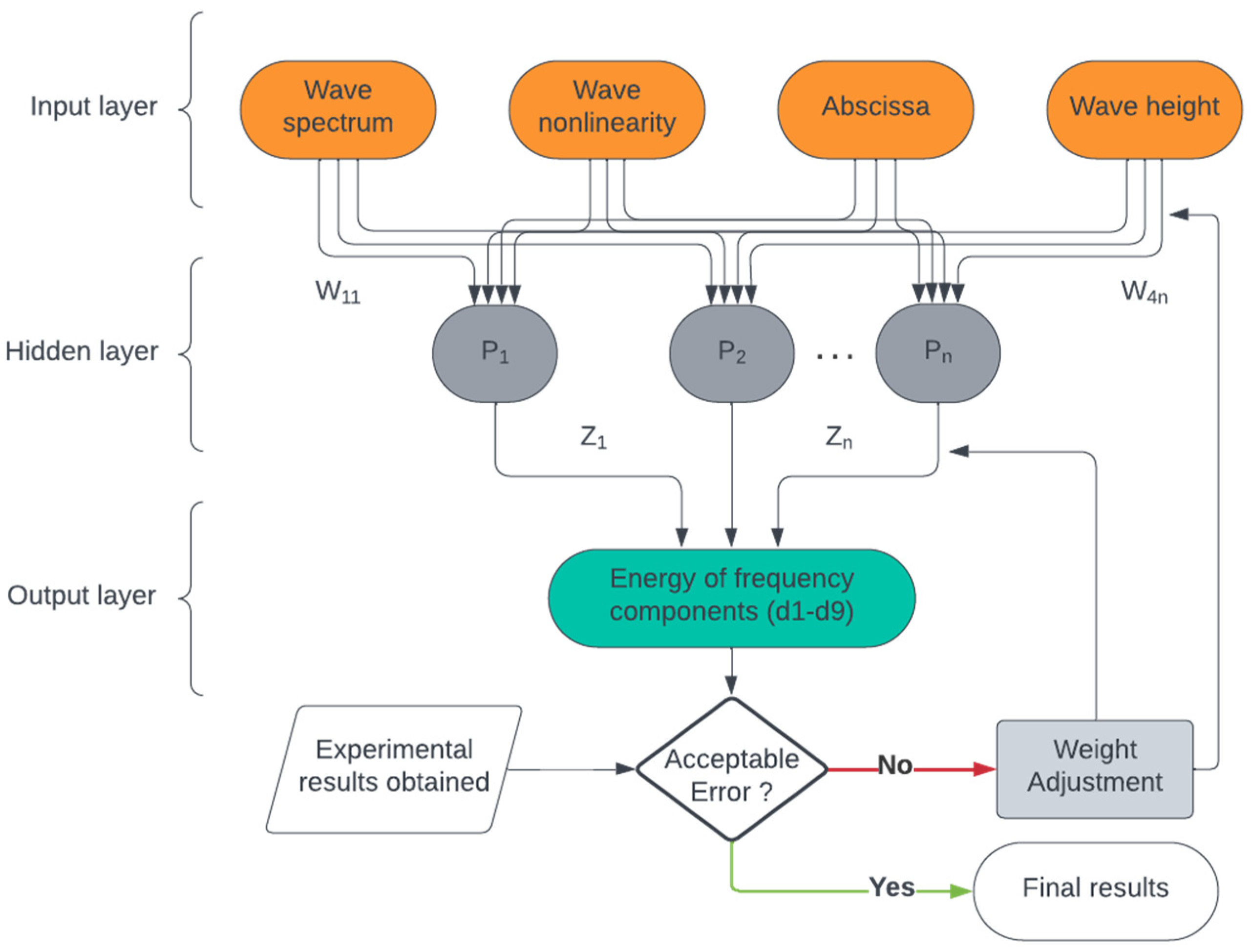
MLP-Regressor is a supervised learning technique that effectively processes information through nonlinear regression by optimizing the squared error. This robust algorithm has already shown its usefulness for various applications [49,50]. It is used to verify the repetitive and accurate nature of our results in forecasting the spatial evolution of frequency component energy. The MLP-Regressor model is structured with three layers, an input layer, a hidden layer containing 100 neurons, and an output layer. Figure 12 shows a simplified schematic diagram of the Multilayer Perceptron (MLP) algorithm. During the training phase, the model is fed input data—including wave spectrum, wave nonlinearity, abscissa along the flume, and water height—to predict the energy values of frequency components (d1–d9). A backpropagation algorithm is then used to minimize the error by adjusting the weights and biases of the network iteratively. This process is repeated for each training example until the network converges to a set of weights and biases that yield low error values for the entire dataset. The programming environment is based on the Python library Scikit-Learn version 0.21.3. To evaluate the model’s performance, R squared (R2) was employed, which yielded a value of 0.935, indicating a high level of fit. Nonetheless, potential areas for improvement include feature engineering, where additional relevant features could be incorporated, and experimenting with different algorithms or hyperparameters to enhance performance. The predictions of two specific frequency components were selected—d5 (Figure 13a) and d8 (Figure 13b)—which exhibited distinguishable variation in Figure 10. The predicted values in grey overlap with the dotted curves obtained experimentally.
Predicting complex dynamic patterns, such as random waves, may be more challenging due to the intricate and nonlinear relationships between different wave features. To improve accuracy and reliability for modeling complex wave dynamics, alternative neural network architectures, such as recurrent neural networks (RNNs) and convolutional neural networks (CNNs), could be considered [51]. Developing accurate predictive capabilities would require access to extensive wave observation data [52]. In addition to traditional wave parameters, such as wave amplitude and frequency, it may be beneficial to consider incorporating other variables, such as spectral bandwidth and wave groupiness, to capture the broader context of wave generation and propagation.
4. Conclusions
When nonlinear waves with sufficient energy encounter each other, they can interact in various ways. Energy dissipation occurs during nonlinear wave–wave interactions, especially in cases of wave breaking, where the wave’s energy is transformed into turbulent kinetic energy and heat due to the chaotic motion of water particles. It was observed that this energy dissipation increased with the nonlinearity . Moreover, the multi-wave train signal investigated in this study showed significantly higher energy levels and a more focused dissipation of energy around the wave breaking area (x ∈ [2,3]) when compared to the single-wave train signal. This observation underscores that the duration of extreme events plays a crucial role in shaping the spatial distribution of energy dissipation. The wavelet transform analysis using the MODWT method provided an additional level of comprehension by identifying particular frequency components related to the process of energy dissipation. This comprehensive frequency decomposition enabled a subtler understanding of the individual contributions of different components of the wave spectrum to dissipation. Based on the wavelet transform analysis, during these nonlinear interactions, energy can be transferred between different frequency components. This work illustrates the effectiveness of the MLP algorithm in enhancing wave prediction based on field experimental data. In the near future, we plan to generate longer signals, such as 100 trains, to gain a more definitive understanding of multi-train generation behavior. We also plan to investigate how environmental factors, such as water depth and seabed composition, influence the observed interactions. Understanding environmental dependencies can enhance the predictive capability of models and contribute to site-specific wave energy management strategies.
Supplementary Materials
The following supporting information can be downloaded at: https://www.mdpi.com/article/10.3390/w16081145/s1.
Author Contributions
Conceptualization, R.M. and N.A.; methodology, R.M., N.A. and E.-I.T.; validation, N.A. and I.A.; formal analysis, R.M.; investigation, R.M.; resources, R.M.; data curation, R.M.; writing—original draft preparation, R.M.; writing—review and editing, R.M, I.A, E.-I.T. and N.A; visualization, R.M.; supervision, N.A., E.-I.T. and N.L.; project administration, N.A.; funding acquisition, N.A. All authors have read and agreed to the published version of the manuscript.
Funding
This research received no external funding.
Data Availability Statement
The free surface elevations files are available in the Supplementary Materials.
Acknowledgments
The authors wish to thank the M2C laboratory for providing research facilities.
Conflicts of Interest
The authors declare no conflicts of interest.
References
- Erikson, L.; Morim, J.; Hemer, M.; Young, I.; Wang, X.L.; Mentaschi, L.; Mori, N.; Semedo, A.; Stopa, J.; Grigorieva, V.; et al. Global ocean wave fields show consistent regional trsends between 1980 and 2014 in a multi-product ensemble. Commun. Earth Environ. 2022, 3, 320. [Google Scholar] [CrossRef]
- Sweet, W.; Hamlington, B.; Kopp, R.E.; Weaver, C.; Barnard, P.L.; Bekaert, D.; Brooks, W.; Craghan, M.; Dusek, G.; Frederikse, T.; et al. Global and Regional Sea Level Rise Scenarios for the United States. Report. 2022. Available online: https://pubs.usgs.gov/publication/70229139 (accessed on 15 April 2024).
- Martello, M.V.; Whittle, A.J. Estimating coastal flood damage costs to transit infrastructure under future sea level rise. Commun Earth Environ. 2023, 4, 137. [Google Scholar] [CrossRef]
- Oppenheimer, M.; Alley, R.B. How high will the seas rise? Science 2016, 354, 1375–1377. [Google Scholar] [CrossRef] [PubMed]
- Petrova, P.; Guedes Soares, C. Maximum wave crest and height statistics of irregular and abnormal waves in an offshore basin. Appl. Ocean Res. 2008, 30, 144–152. [Google Scholar] [CrossRef]
- Abroug, I.; Abcha, N.; Dutykh, D.; Jarno, A.; Marin, F. Experimental and numerical study of the propagation of focused wave groups in the nearshore zone. Phys. Lett. A 2020, 384, 126144. [Google Scholar] [CrossRef]
- Abroug, I.; Abcha, N.; Jarno, A.; Marin, F. Laboratory study of non-linear wave–wave interactions of extreme focused waves in the nearshore zone. Nat. Hazards Earth Syst. Sci. 2020, 20, 3279–3291. [Google Scholar] [CrossRef]
- Onorato, M.; Residori, S.; Bortolozzo, U.; Montina, A.; Arecchi, F.T. Rogue waves and their generating mechanisms in different physical contexts. Phys. Rep. 2013, 528, 47–89. [Google Scholar] [CrossRef]
- Kharif, C.; Pelinovsky, E. Physical mechanisms of the rogue wave phenomenon. Eur. J. Mech.—B/Fluids 2003, 22, 603–634. [Google Scholar] [CrossRef]
- Whittaker, C.N.; Fitzgerald, C.J.; Raby, A.C.; Taylor, P.H.; Borthwick, A.G.L. Extreme coastal responses using focused wave groups: Overtopping and horizontal forces exerted on an inclined seawall. Coast. Eng. 2018, 140, 292–305. [Google Scholar] [CrossRef]
- Baldock, T.E.; Swan, C.; Taylor, P.H. A laboratory study of nonlinear surface waves on water. Phil. Trans. R. Soc. Lond. A 1996, 354, 649–676. [Google Scholar] [CrossRef]
- Rapp, R.J.; Melville, W.K. Laboratory measurements of deep-water breaking waves. Phil. Trans. R. Soc. Lond. A 1990, 331, 735–800. [Google Scholar] [CrossRef]
- Wu, C.H.; Nepf, H.M. Breaking criteria and energy losses for three-dimensional wave breaking. J. Geophys. Res. 2002, 107, 41-1–41-18. [Google Scholar] [CrossRef]
- Yao, A.; Wu, C.H. Spatial and Temporal Characteristics of Transient Extreme Wave Profiles on Depth-Varying Currents. J. Eng. Mech. 2006, 132, 1015–1025. [Google Scholar] [CrossRef]
- Dysthe, K.; Krogstad, H.E.; Müller, P. Oceanic Rogue Waves. Annu. Rev. Fluid Mech. 2008, 40, 287–310. [Google Scholar] [CrossRef]
- Zhang, J.; Benoit, M.; Kimmoun, O.; Chabchoub, A.; Hsu, H.-C. Statistics of Extreme Waves in Coastal Waters: Large Scale Experiments and Advanced Numerical Simulations. Fluids 2019, 4, 99. [Google Scholar] [CrossRef]
- Trulsen, K.; Zeng, H.; Gramstad, O. Laboratory evidence of freak waves provoked by non-uniform bathymetry. Phys. Fluids 2012, 24, 097101. [Google Scholar] [CrossRef]
- Kashima, H.; Hirayama, K.; Mori, N. Estimation of freak wave occurrence from deep to shallow water regions. In Proceedings of the 34th International Conference on Coastal Engineering (ICCE 2014), Seoul, Republic of Korea, 15–20 June 2014; Volume 1. [Google Scholar] [CrossRef]
- Massel, S.R. Wavelet analysis for processing of ocean surface wave records. Ocean Eng. 2001, 28, 957–987. [Google Scholar] [CrossRef]
- Fu, R.; Ma, Y.; Dong, G.; Perlin, M. A wavelet-based wave group detector and predictor of extreme events over unidirectional sloping bathymetry. Ocean Eng. 2021, 229, 108936. [Google Scholar] [CrossRef]
- Percival, D.B.; Walden, A.T. Wavelet Methods for Time Series Analysis; Cambridge University Press: Cambridge, UK, 2000; ISBN 978-0-511-84104-0. [Google Scholar]
- Cornish, C.R.; Bretherton, C.S.; Percival, D.B. Maximal Overlap Wavelet Statistical Analysis with Application to Atmospheric Turbulence. Bound.-Layer Meteorol. 2006, 119, 339–374. [Google Scholar] [CrossRef]
- Günaydın, K. The estimation of monthly mean significant wave heights by using artificial neural network and regression methods. Ocean Eng. 2008, 35, 1406–1415. [Google Scholar] [CrossRef]
- Malekmohamadi, I.; Bazargan-Lari, M.R.; Kerachian, R.; Nikoo, M.R.; Fallahnia, M. Evaluating the efficacy of SVMs, BNs, ANNs and ANFIS in wave height prediction. Ocean Eng. 2011, 38, 487–497. [Google Scholar] [CrossRef]
- James, S.C.; Zhang, Y.; O’Donncha, F. A machine learning framework to forecast wave conditions. Coast. Eng. 2018, 137, 1–10. [Google Scholar] [CrossRef]
- Rynkiewicz, J. General bound of overfitting for MLP regression models. Neurocomputing 2012, 90, 106–110. [Google Scholar] [CrossRef]
- White, H. Artificial Neural Networks: Approximation and Learning Theory; Blackwell Publishers, Inc.: Malden, MA, USA, 1992; ISBN 1-55786-329-6. [Google Scholar]
- Akkaya, B.; Çolakoğlu, N. Comparison of Multi-Class Classification Algorithms on Early Diagnosis of Heart Diseases. In Proceedings of the y-BIS 2019 Conference: ISBIS Young Business and Industrial Statisticians Workshop on Recent Advances in Data Science and Business Analytics, Istanbul, Turkey, 25–28 September 2019. [Google Scholar]
- Dutt, M.I.; Saadeh, W. A Multilayer Perceptron (MLP) Regressor Network for Monitoring the Depth of Anesthesia. In Proceedings of the 2022 20th IEEE Interregional NEWCAS Conference (NEWCAS), Quebec City, QC, Canada, 19–22 June 2022; pp. 251–255. [Google Scholar]
- Abroug, I.; Matar, R.; Abcha, N. Spatial Evolution of Skewness and Kurtosis of Unidirectional Extreme Waves Propagating over a Sloping Beach. J. Mar. Sci. Eng. 2022, 10, 1475. [Google Scholar] [CrossRef]
- Xu, J.; Liu, S.; Li, J.; Jia, W. Experimental study of wave height, crest, and trough distributions of directional irregular waves on a slope. Ocean Eng. 2021, 242, 110136. [Google Scholar] [CrossRef]
- Adcock, T.A.A.; Taylor, P.H. Estimating ocean wave directional spreading from an Eulerian surface elevation time history. Proc. R. Soc. A 2009, 465, 3361–3381. [Google Scholar] [CrossRef]
- Tromans, P.; Anaturk, A.R.; Hagemeijer, P. A new model for the kinematics of large ocean waves-application as a design wave. In Proceedings of the ISOPE International Ocean and Polar Engineering Conference, Edinburgh, UK, 11–16 August 1991; Volume 3. [Google Scholar]
- Whittaker, C.N.; Fitzgerald, C.J.; Raby, A.C.; Taylor, P.H.; Orszaghova, J.; Borthwick, A.G.L. Optimisation of focused wave group runup on a plane beach. Coast. Eng. 2017, 121, 44–55. [Google Scholar] [CrossRef]
- Beji, S. Note on a nonlinearity parameter of surface waves. Coast. Eng. 1995, 25, 81–85. [Google Scholar] [CrossRef]
- Pierson, W.J.; Moskowitz, L. A proposed spectral form for fully developed wind seas based on the similarity theory of S. A. Kitaigorodskii. J. Geophys. Res. 1964, 69, 5181–5190. [Google Scholar] [CrossRef]
- Hasselmann, K.; Barnett, T.; Bouws, E.; Carlson, H.; Cartwright, D.; Enke, K.; Ewing, J.; Gienapp, H.; Hasselmann, D.; Kruseman, P.; et al. Measurements of wind-wave growth and swell decay during the Joint North Sea Wave Project (JONSWAP). Deut. Hydrogr. Z. 1973, 8, 1–95. [Google Scholar]
- Craciunescu, C.C.; Christou, M. Wave breaking energy dissipation in long-crested focused wave groups based on JONSWAP spectra. Appl. Ocean Res. 2020, 99, 102144. [Google Scholar] [CrossRef]
- Rezaie-balf, M.; Naganna, S.R.; Ghaemi, A.; Deka, P.C. Wavelet coupled MARS and M5 Model Tree approaches for groundwater level forecasting. J. Hydrol. 2017, 553, 356–373. [Google Scholar] [CrossRef]
- Mouatadid, S.; Adamowski, J.F.; Tiwari, M.K.; Quilty, J.M. Coupling the maximum overlap discrete wavelet transform and long short-term memory networks for irrigation flow forecasting. Agric. Water Manag. 2019, 219, 72–85. [Google Scholar] [CrossRef]
- Quilty, J.; Adamowski, J. Addressing the incorrect usage of wavelet-based hydrological and water resources forecasting models for real-world applications with best practices and a new forecasting framework. J. Hydrol. 2018, 563, 336–353. [Google Scholar] [CrossRef]
- Massei, N.; Dieppois, B.; Hannah, D.M.; Lavers, D.A.; Fossa, M.; Laignel, B.; Debret, M. Multi-time-scale hydroclimate dynamics of a regional watershed and links to large-scale atmospheric circulation: Application to the Seine river catchment, France. J. Hydrol. 2017, 546, 262–275. [Google Scholar] [CrossRef]
- Turki, E.I.; Deloffre, J.; Lecoq, N.; Gilbert, R.; Mendoza, E.T.; Laignel, B.; Salameh, E.; Gutierrez Barcelo, A.D.; Fournier, M.; Massei, N. Multi-timescale dynamics of extreme river flood and storm surge interactions in relation with large-scale atmospheric circulation: Case of the Seine estuary. Estuar. Coast. Shelf Sci. 2023, 287, 108349. [Google Scholar] [CrossRef]
- Rahman, A.T.M.S.; Hosono, T.; Quilty, J.M.; Das, J.; Basak, A. Multiscale groundwater level forecasting: Coupling new machine learning approaches with wavelet transforms. Adv. Water Resour. 2020, 141, 103595. [Google Scholar] [CrossRef]
- Osborne, A.R. Harmonic Generation in Shallow-Water Waves. In International Geophysics; Elsevier: Amsterdam, The Netherlands, 2010; Volume 97, pp. 795–817. ISBN 978-0-12-528629-9. [Google Scholar]
- Wu, Q.; Feng, X.; Dong, Y.; Dias, F. On the behavior of higher harmonics in the evolution of nonlinear water waves in the presence of abrupt depth transitions. Phys. Fluids 2023, 35, 127102. [Google Scholar] [CrossRef]
- Zhang, S. Energy and momentum dissipation through wave breaking. J. Geophys. Res. 2005, 110, C09021. [Google Scholar] [CrossRef]
- Padilla, E.M.; Alsina, J.M. Transfer and dissipation of energy during wave group propagation on a gentle beach slope. JGR Ocean. 2017, 122, 6773–6794. [Google Scholar] [CrossRef]
- Qin, Y.; Li, C.; Shi, X.; Wang, W. MLP-Based Regression Prediction Model For Compound Bioactivity. Front. Bioeng. Biotechnol. 2022, 10, 946329. [Google Scholar] [CrossRef] [PubMed]
- Maqbool, J.; Aggarwal, P.; Kaur, R.; Mittal, A.; Ganaie, I.A. Stock Prediction by Integrating Sentiment Scores of Financial News and MLP-Regressor: A Machine Learning Approach. Procedia Comput. Sci. 2023, 218, 1067–1078. [Google Scholar] [CrossRef]
- Domala, V.; Lee, W.; Kim, T. Wave data prediction with optimized machine learning and deep learning techniques. J. Comput. Des. Eng. 2022, 9, 1107–1122. [Google Scholar] [CrossRef]
- Durap, A. A comparative analysis of machine learning algorithms for predicting wave runup. Anthr. Coasts 2023, 6, 17. [Google Scholar] [CrossRef]
Figure 1.
Sketch of the wave flume. The direction of propagation from left to right.

Figure 2.
Reference wave gauge (WGR) signals for three different spectra, namely Pierson–Moskowitz, JONSWAP (γ = 3.3), and JONSWAP (γ = 7), using one, three, six, and nine wave trains.
Figure 2.
Reference wave gauge (WGR) signals for three different spectra, namely Pierson–Moskowitz, JONSWAP (γ = 3.3), and JONSWAP (γ = 7), using one, three, six, and nine wave trains.

Figure 3.
Spatial evolution of the spectrum and spectra of three positions using a signal of one wave train and for (a,b) Pierson–Moskowitz (γ = 1) spectrum; (c,d) JONSWAP (γ = 3.3) spectrum; and (e,f) JONSWAP (γ = 7) spectrum, respectively.
Figure 3.
Spatial evolution of the spectrum and spectra of three positions using a signal of one wave train and for (a,b) Pierson–Moskowitz (γ = 1) spectrum; (c,d) JONSWAP (γ = 3.3) spectrum; and (e,f) JONSWAP (γ = 7) spectrum, respectively.

Figure 4.
Spatial evolution of the spectrum and spectra of three positions using a signal of nine wave trains and for (a,b) Pierson–Moskowitz (γ = 1) spectrum; (c,d) JONSWAP (γ = 3.3) spectrum; and (e,f) JONSWAP (γ = 7) spectrum, respectively. (Spectra of Figure 3, using a signal of one wave train are represented by dashed lines).

Figure 5.
Individual dimensionless energy evolution of nine wave trains.

Figure 6.
Energy dissipation percentage using a signal of one wave train and several nonlinearities for (a) Pierson–Moskowitz (γ = 1) spectrum, (b) JONSWAP (γ = 3.3) spectrum, and (c) JONSWAP (γ = 7) spectrum.
Figure 6.
Energy dissipation percentage using a signal of one wave train and several nonlinearities for (a) Pierson–Moskowitz (γ = 1) spectrum, (b) JONSWAP (γ = 3.3) spectrum, and (c) JONSWAP (γ = 7) spectrum.

Figure 7.
Energy dissipation percentage using a signal of nine wave trains and several nonlinearities for (a) Pierson–Moskowitz (γ = 1) spectrum, (b) JONSWAP (γ = 3.3) spectrum, and (c) JONSWAP (γ = 7) spectrum.
Figure 7.
Energy dissipation percentage using a signal of nine wave trains and several nonlinearities for (a) Pierson–Moskowitz (γ = 1) spectrum, (b) JONSWAP (γ = 3.3) spectrum, and (c) JONSWAP (γ = 7) spectrum.

Figure 8.
Free surface elevation of the reference wave gauge WGR using a JONSWAP (γ = 3.3) signal of nine wave trains and = 0.82.
Figure 8.
Free surface elevation of the reference wave gauge WGR using a JONSWAP (γ = 3.3) signal of nine wave trains and = 0.82.

Figure 9.
Frequency components of the reference signal ranging from d1 to d9, with the dominant components being d5 (the peak frequency) and d4 (harmonic frequency).
Figure 9.
Frequency components of the reference signal ranging from d1 to d9, with the dominant components being d5 (the peak frequency) and d4 (harmonic frequency).

Figure 10.
Spatial evolution of frequency component energy using a JONSWAP (γ = 3.3) signal of nine wave trains and = 0.82. (, , , , , , , , ).
Figure 10.
Spatial evolution of frequency component energy using a JONSWAP (γ = 3.3) signal of nine wave trains and = 0.82. (, , , , , , , , ).

Figure 11.
Spatial evolution of six frequency components’ (d4–d9) energy differential using a JONSWAP (γ = 3.3) signal of nine wave trains and several nonlinearities.
Figure 11.
Spatial evolution of six frequency components’ (d4–d9) energy differential using a JONSWAP (γ = 3.3) signal of nine wave trains and several nonlinearities.

Figure 12.
A simplified schematic diagram of the Multilayer Perceptron (MLP) model showing the input, hidden, and output layers.
Figure 12.
A simplified schematic diagram of the Multilayer Perceptron (MLP) model showing the input, hidden, and output layers.

Figure 13.
The spatial evolution of (a) d5 and (b) d8 for a JONSWAP (γ = 3.3) signal of nine wave trains using several nonlinearities. The experimental results are represented by dotted curves, while the predicted results are shown by the grey continuous line.
Figure 13.
The spatial evolution of (a) d5 and (b) d8 for a JONSWAP (γ = 3.3) signal of nine wave trains using several nonlinearities. The experimental results are represented by dotted curves, while the predicted results are shown by the grey continuous line.


Table 1.
Experimental parameters used.
| Spectrum | PIERSON–MOSKOWITZ | JONSWAP (γ = 3.3) | JONSWAP (γ = 7) |
|---|---|---|---|
| Peak frequency fp | 0.75 Hz | 0.75 Hz | 0.75 Hz |
| 0.16 | 0.20 | 0.24 | |
| 0.20 | 0.25 | 0.30 | |
| 0.23 | 0.30 | 0.36 | |
| 0.27 | 0.35 | 0.42 | |
| 0.31 | 0.40 | 0.47 | |
| 0.35 | 0.44 | 0.52 | |
| 0.39 | 0.47 | 0.57 | |
| 0.43 | 0.53 | - | |
| 0.47 | 0.57 | - | |
| Number of trains | 1–3–6–9 | 1–3–6–9 | 1–3–6–9 |
| WG positions | 51 | 51 | 51 |
Disclaimer/Publisher’s Note: The statements, opinions and data contained in all publications are solely those of the individual author(s) and contributor(s) and not of MDPI and/or the editor(s). MDPI and/or the editor(s) disclaim responsibility for any injury to people or property resulting from any ideas, methods, instructions or products referred to in the content. |
© 2024 by the authors. Licensee MDPI, Basel, Switzerland. This article is an open access article distributed under the terms and conditions of the Creative Commons Attribution (CC BY) license (https://creativecommons.org/licenses/by/4.0/).
Share and Cite
MDPI and ACS Style
Matar, R.; Abcha, N.; Abroug, I.; Lecoq, N.; Turki, E.-I. A Multi-Approach Analysis for Monitoring Wave Energy Driven by Coastal Extremes. Water 2024, 16, 1145. https://doi.org/10.3390/w16081145
AMA Style
Matar R, Abcha N, Abroug I, Lecoq N, Turki E-I. A Multi-Approach Analysis for Monitoring Wave Energy Driven by Coastal Extremes. Water. 2024; 16(8):1145. https://doi.org/10.3390/w16081145
Chicago/Turabian StyleMatar, Reine, Nizar Abcha, Iskander Abroug, Nicolas Lecoq, and Emma-Imen Turki. 2024. "A Multi-Approach Analysis for Monitoring Wave Energy Driven by Coastal Extremes" Water 16, no. 8: 1145. https://doi.org/10.3390/w16081145
Note that from the first issue of 2016, this journal uses article numbers instead of page numbers. See further details here.