Parameter Optimization of Frazil Ice Evolution Model Based on NSGA-II Genetic Algorithm

1
State Key Laboratory of Hydraulic Engineering Intelligent Construction and Operation, Tianjin University, Tianjin 300072, China
2
School of Civil Engineering, Tianjin University, Tianjin 300072, China
3
Institute of Ocean Energy and Intelligent Construction, Tianjin University of Technology, Tianjin 300382, China
*
Author to whom correspondence should be addressed.
Water 2024, 16(9), 1232; https://doi.org/10.3390/w16091232
Submission received: 26 March 2024
/
Revised: 21 April 2024
/
Accepted: 23 April 2024
/
Published: 25 April 2024
Abstract
:This study is based on the research results of frazil ice evolution in recent years and proposes an improved frazil ice evolution mathematical model. Based on the NSGA-II genetic algorithm, seven key parameters were used as optimization design variables, the minimum average difference between the number of frazil ice, the mean and the standard deviation of particle diameter of the simulation results, and the observed data were used as the optimization objective, the Pareto optimal solution set was optimized, and the importance of each objective function was analyzed and discussed. The results show that compared to previous models, the improved model has better agreement between simulation results and experimental results. The optimal parameters obtained by the optimization model reduces the difference rate of water temperature process by 5.75%, the difference rate of quantity process by 39.13%, the difference rate of mean particle size process by 47.64%, and the difference rate of standard deviation process by 56.84% during the period of intense evolution corresponding to the initial parameter group. The results prove the validity of the optimization model of frazil ice evolution parameters.
1. Introduction
The formation and evolution of frazil ice is a natural phenomenon in rivers and channels in cold regions and is the basis for all ice problems. It is of great significance to study and simulate the evolution and development process of frazil ice in order to ensure the safe operation of water conservancy projects and give full play to the benefits of water conservancy projects.
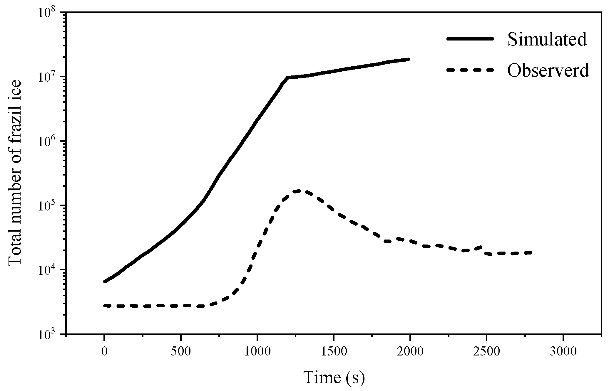
A few mathematical models have been developed to simulate frazil ice evolution [1]. Omstedt and Svensson [2] formulated and explored a mathematical model for studying supercooling and ice formation in turbulent waters based on the conservation equations in their one-dimensional form. This model is an extension of the model presented by Osterkamp and Gosink [3]. Svensson and Omstedt [4] developed a mathematical model based on the physical processes available at the time, including initial seeding, secondary nucleation, gravity removal, thermal growth, and flocculation/breakup. This model was subsequently refined by Wang and Doering [5]. Hammar and Shen [6] developed a model for the formation and evolution of frazil in open channels that examined the effects of surface heat exchange, seeding rates, rate of secondary nucleation, and flow conditions on the evolution. Doering [7,8] developed a model to simulate the principal supercooling process and evolution of frazil ice particles in a counter-rotating flume flow, in which only the overall heat balance was considered for the entire process. Although the model mentioned above includes a relatively complete process of frazil ice evolution, several differences remain between the calculated and actual observational results. Taking the frazil ice evolution model proposed by Wang and Doering [5] as an example, the calculated amount of frazil ice showed a continuous increase during the evolution process; however, in actual observations, the amount initially increased and then decreased (Figure 1).
The authors analyzed and summarized the latest experimental observation results in recent years, proposing an improved frazil ice evolution mathematical model. Some new parameters are proposed in this model, and the changes in them significantly affect the calculation results; for example, the water-outside heat exchange coefficient hwa and the ice nucleation formation coefficient k affect the change process of water temperature, the thickness-to-width ratio Std affects the change process of mean and standard deviation of the frazil ice particle size, and the stable particle size range and the collision calibration coefficient affect the change process of the quantity, etc. Compared with the previous model, the agreement between the calculated results and the experimental observation results is greatly improved. However, it is difficult to determine some key parameter values in order to better match the model calculation results with the experimental results, as the simulation results are influenced by two or even more parameters taken together. Therefore, this study requires collaborative optimization of the model parameters. In recent years, researchers have used various methods to optimize observed, collected, or simulated data for better results [9,10,11,12,13], including but not limited to machine-learning, deep-learning, and multi-objective optimization algorithms. The problem of this study focuses on how the parameters should be valued so that the results of the model calculations of the evolution of frazil ice best fit the experimental observations. The parameters include hwa, k, and other parameters mentioned above, and the results of the numerical modeling are the water temperature, the number of frazil ice particles, and the mean and standard deviation of particle diameter. Therefore, this study is a multi-objective optimization problem. Multi-objective optimization genetic algorithms are widely developed and applied for such problems. The non-dominated sorting genetic algorithm (NSGA) proposed by Srinivas and Deb [14] is one of the earliest such evolutionary algorithms. However, this algorithm has been criticized by scholars for its high computational complexity, lack of elitism, and the need to specify the shared radius artificially. Therefore, Deb et al. [15] proposed the NSGA- II algorithm in 2000. The main improvements are in terms of computational efficiency, the use of an elite strategy, and the use of a crowding comparison operator to retain the best individuals and a uniform distribution. The NSGA-II algorithm has been improved over the NSGA algorithm both in terms of optimization effect and computing time, which is an excellent multi-objective optimization algorithm and is now widely used in various fields [16,17,18,19,20]. However, it has been shown empirically that NSGA-II does not scale well with an increasing number of objectives [21,22,23,24]. Lücken et al. [25] and Li et al. [26] also pointed out the limitations of the crowded comparison operator used by NSGA-II when solving multi-objective optimization problems with more objectives. Further, Deb and Jain [27] proposed an evolutionary multi-target, called NSGA-III, which uses a reference-point-based selection method to select individuals into the next generation. However, Ishibuchi et al. [28] showed that NSGA-III does not always perform better than NSGA-II by comparing various multi-objective test problems. Given that there are not more than four objectives in this study, taking into account the optimization efficiency and reliability, the NSGA-II genetic algorithm is used in this study to optimize the parameters of the in-water ice evolution model.
Based on this, this study first presents an improved mathematical model for the evolution of frazil ice based on the results of recent laboratory experiments and field observations. Then, the authors take the observation data of ice in a turbulent glass tank in a low temperature room conducted by Mcfarlane [29] as reference and seven parameters including ice nucleation formation coefficient k, upper limit DB-max and lower limit DB-min of stable particle size interval, thickness-to-width ratio Std, initial value of collision frequency calibration coefficient sequences M1, collision fragmentation calibration coefficient KB, and KC as optimization variables. Taking the average difference rate of the simulation results of the number of frazil ice and the mean particle size and standard deviation compared with the observed data as the optimization objective, the NSGA-II genetic algorithm was used to establish a multi-objective optimization model to quickly determine the parameters of the evolution model of frazil ice, and the Pareto optimal solution set was optimized. The simulation results corresponding to the optimal parameters in the solution set were compared with the corresponding results of the initial parameter set to verify the effectiveness of the optimization model.
2. Model Formulation
A box cell with well-mixed water and frazil ice was calculated in the model. The frazil ice particles were divided into N equally varying particle size groups, assuming that each group was of equal size. Frazil ice nuclei were assumed to be in the smallest size group. The number of particles ni in each group is a function of nucleation, thermal growth, collision flocculation and breakup, and gravitational removal and can be described by the number continuity equation as follows:
where i is the particle size group number and i = 1 represents the ice nuclei group; is the number of particles in the i-th particle size group. The subscript represents the change in the quantity of the first group due to nucleation and the subscripts , , , , and represent the changes in the quantity of the i-th group due to thermal growth, collision, flocculation, breakup and gravitational removal, respectively.
2.1. Heat Exchanges and Water Temperature
The water temperature was obtained using the following heat balance equation:
where is water density; is the water specific heat capacity; is the volume concentration of frazil ice; is water temperature; is the heat exchange flux between water and air; is heat exchange flux between water and ice; and i is frazil grouping number (1, 2, …, N); is the area of heat exchange between the water and air; is the heat transfer coefficient between the water and air, which is determined by specific conditions; is the air temperature; is heat transfer coefficient between water and ice, and can be expressed by the Nusselt number, which can be found in Holland [30].
2.2. Initial Seeding
The initial seeding is the trigger condition for the operation of a frazil ice evolution model. In previous models, this process was treated in a simplified manner [5], which cannot be applied in practical situations. The past studies show that frazil ice production in nature involves heterogeneous nucleation [31,32,33,34], and the rate of ice nucleation is closely related to weather conditions (rainfall, snowfall, and high winds) and water temperature. An equation for the rate of ice nucleation based on the power function form is proposed:
where is the amount of ice core generation and k is the coefficient, which is obtained by calibrating weather conditions, such as clear and windless, rainfall, and snowfall.
2.3. Ice Particle Growth
The change in the volume of ice produced by crystal growth per unit time in the i-th radius interval is [5]
where is the amount of change in volume of ice in the i-th radius interval; is ice density; is latent heat of ice fusion; and is active area per ice particle, i.e., the area of frazil ice. According to existing studies, frazil ice is of the thin-disc type, and the observed thickness-to-width ratio, Std = ti/D, ranges from 1/10 to 1/100. ti is the thickness of an ice particle, and Di is the diameter.
2.4. Ice Particle Collision Frequency
Collisions between particles are another important component in the evolution of frazil ice. The process of flocculation and breakup caused by collisions is an important component of the evolution of frazil ice. This study proposed a method to calculate the occurrence of ice collision events for each particle size group, which draws on the theory of random collisions of solid particles in gas–solid two-phase flows. Before the collision began, colliding particle group i was selected, the particle size and velocity of motion were determined, and the number of collisions in the group could be determined by the average collision frequency. The distance traveled by particle group i in time dt is , and the corresponding cylinder volume is . The collision frequency of particle group i with other particles in time dt can be obtained by
The particles in the above equation move along the direction normal to the bottom of the thin disk from the beginning to the end (Figure 2a), and the resulting volume of motion is a cylinder; however, in practice, this motion of ice in water cannot exist because frazil ice is affected by the flow of water rotational motion (Figure 2b). Therefore, a calibration factor, , is introduced in the frazil ice collision frequency, where M1 is the calibration coefficient of the smallest particle-size group particle collision frequency. The large frazil ice is mostly flocculated; therefore, the larger the size of the body is closer to the sphere, the larger is Mi. MN = 1, and N is the group of particles with the largest size.
Therefore, the total collision frequency of group i ice particles at time dt is
After determining that the colliding particles collided with other particles, the group of collided particles (particle size, velocity, etc.) was selected using the following steps:
(1) The particle size and number of ice particles was identified in the current computational body. For example, the total number of particles in computational cell C is nt, and ni particles with particle size Di exist in the i-th group.
(2) The ratio of the number of each particle size group to the total number in the calculation cell C is
(3) A random number rn between [0, 1] was selected, and the virtual particle size was selected as follows:
where j is the number of collided particle groups and is the particle diameter of the j-th group.
From this, the particle size and velocity of the particles involved in the collision can be determined, and the result of the collision, flocculation or breakup (secondary nucleation) can be determined.
2.5. Flocculation/Breakup
It is indeed challenging to ascertain the flocculation or breakup process of frazil ice particles after collision [6], with previous models often undergoing simplification [2,4,5]. In recent years, scholars have simulated the evolution process of frazil ice through physical models, and obtained intuitive observation results and the time history changes and of water temperature, particles quantity, mean particle size, and standard deviation. Drawing upon these experimental findings, this article conducts an analysis of the flocculation and breakup processes of frazil ice.
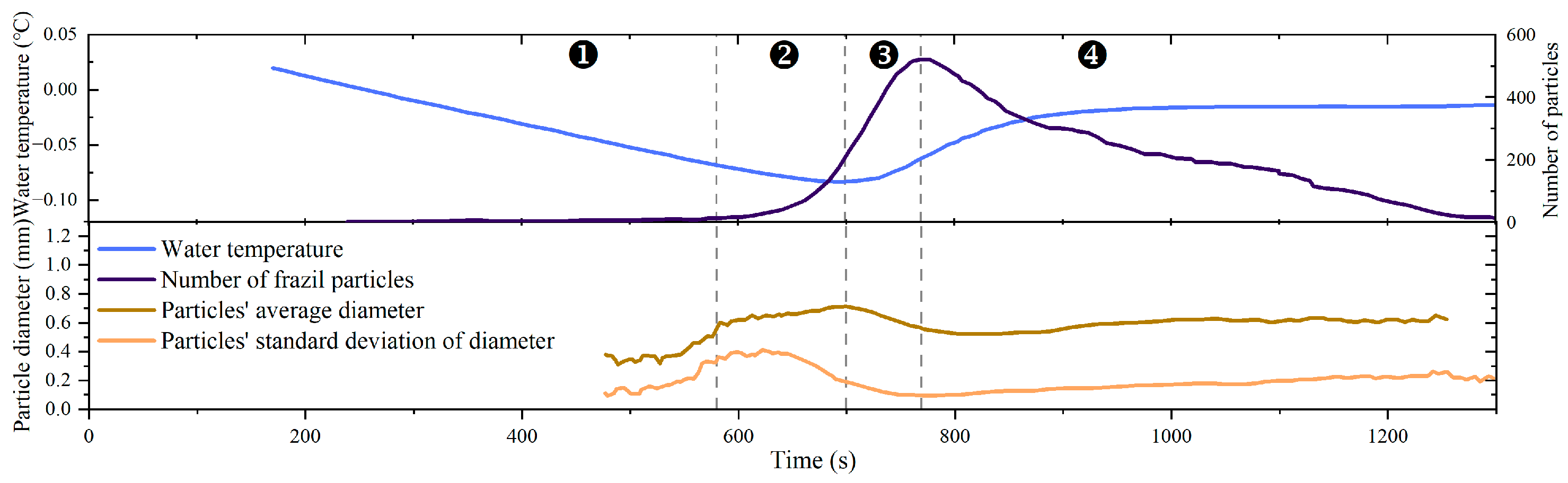
Taking the 2015 MacFarlane’s experiment as an example, Figure 3 shows the water temperature, frazil ice quantity, and mean and standard deviation of particle diameter collected under turbulent dissipation rate conditions of 335.6 cm2/s3. Based on the change points of these curves, the evolution process is divided into four stages:
(1) At the first stage, the amount and size of frazil ice is small, and the probability of collision is extremely low. At this time, thermal growth is the main factor.
(2) The rate of increase in the amount of frazil ice increased significantly in second stage, and it entered the “explosive” growth stage, which means that the role of secondary nucleation begins to appear. Based on published images of frazil ice, flocs are formed by the flocculation of particles with large size differences, and small particles have a high probability of flocculation after collision with other-sized particles. Particles of similar sizes have a high probability of breaking when they collide with each other because of their similar strength and motion, that is, secondary nucleation processes. Further analysis suggests that large particles are mostly generated by flocculation and have a sparse structure; therefore, the breakup process most likely occurs between large particles.
(3) The number of frazil ice particles in the third stage was larger, leading to an increase in the collision frequency, and secondary nucleation and flocculation effects were evident. Secondary nucleation led to a continued increase in the amount of frazil ice; flocculation promoted the production of large flocs.
(4) At the fourth stage, the amount of frazil ice began to decrease, and the mean and standard deviation of the particle diameters gradually approached a steady state. During this period, the large particles continued to float and be removed in the region, reducing their number; thus, the frequency of large particle collisions was reduced, and the secondary nucleation effect was weakened.
The above process also shows a similar trend in Clark’s experimental results [35,36]. Based on laboratory observations, the size distribution of ice particles maintained a normal distribution during the evolution of frazil ice [29], which indicated that there were many particles within a certain size range, and the probability of particles colliding with each other within this range was also high. If flocculation of breakup occurred, it easily affected the stable state of the mean value and standard deviation at the end of the evolution. Therefore, we assume that there is a certain particle size range, and it is likely that no flocculation and breakup occurs between the ice particles within this range, but rather they bounce apart after colliding like “elastic bodies”.
Based on the above analysis, it is presumed that the development of frazil ice after collision is primarily controlled by the particle size under flow conditions such as turbulence intensity. The frazil ice was divided into three particle size ranges: A, B, and C, ranging from small to large (Figure 4). Group B is called the stable particle size group. Based on the above analysis, collision between particles in the B interval and B interval (referred to as the “BB” interval particles collision, the same below) likely does not cause flocculation or breakup, The frazil ice within the same particle size range collision, i.e., “AA” collisions with “CC” collisions, where secondary nucleation occurs, and collisions of small grains with larger grains, i.e., “AB” collisions, “AC” and “AB” collisions, and “AC” and “BC” collisions, result in flocculation. The key variables, the upper and lower limit of the stable particle size range, are denoted as Da and Db, respectively. However, the judgment of each of the above results is not absolute, as collision results are a complex process influenced by many factors. The breakup calibration coefficients KB (KB ≤ 1) and KC (KC ≤ 1) are introduced into the calculation of the number of particles generated in the BB and CC interval particle collisions.
2.6. Gravitational Removal
Gravitational removal means that the frazil ice is buoyantly brought to the surface and no longer enters the computational domain, assuming that the water–air heat exchange is not affected. The rising speed of ice was based on the rise velocities measured by Matoušek [37]:
3. NSGA-II Non-Dominated Sorting Genetic Algorithm
3.1. Optimization Parameters and Objective Function Equation
The above model contains parameters that cannot be accurately determined, including ice nucleation formation coefficient k, upper limit DB-max, and lower limit DB-min of stable particle size interval, thickness-to-width ratio Std, initial value of collision frequency calibration coefficient sequences M1, and collision fragmentation calibration coefficients KB and KC. The thickness-to-width ratio is related to the volume and diameter of particles, which in turn affects the variation of particle size. Therefore, it is also a parameter that needs to be considered. Before optimizing the parameters, we conducted preliminary calculations during the model establishment and improvement stage, and thus determined the appropriate range of values for these parameters. These parameters were taken as optimization variables, among which the parameters and constraint interval are shown in Table 1 as follows:
Specifically, the objective of the optimization of the model in this study is to minimize the average difference value between the amount of frazil ice, the average particle diameter, and the standard deviation of diameter calculated by the model compared with the experimental observation results through reasonable values of seven variables, so the objective function is as follows:
where X represents seven optimization design parameters, are the number of frazil ice, average particle diameter and standard deviation of diameter calculated by the model in the evolution process; are frazil ice data from experimental observations; t is the time; and T is the total time.
3.2. A Fast Non-Dominated Sorting Approach
A fast non-dominated sorting approach is a concept proposed on the basis of Pareto domination. For the optimal design parameter X in this paper, if there exists for individuals X1 and X2 for any objective function, then individual X1 dominates X2; X1 is said to weakly dominate X2 if there exists for any objective function and at least one objective function such that holds.; individuals X1 and X2 are said to be mutually nondominant if there exists both an objective function such that holds and an objective function that satisfies . The non-dominating level is also called Pareto level, in which the individual with Pareto level 1 is called the non-dominating solution, also called the Pareto optimal solution, and the curve formed by the solution set is called the Pareto frontier.
The steps of fast non-dominated ranking are as follows [15]:
(1) For each individual in the solution set, calculate its two variable values: the dominated number np and the dominated set Sp;
(2) Find all the individuals np = 0 in the solution set, assign their non-dominant rank prank = 1, and store these individuals in the non-dominant set F(1);
(3) For each individual in the set F(1), the dominant number ni of each individual p in the set Sp is subtracted by 1. If ni − 1 = 0, the individual p is placed in the set F(2), and the individual p in the set is assigned the non-dominant rank prank = 2;
(4) Then repeat the above operation for each individual in the set F(2) until all individuals have been assigned a non-dominant rank.
3.3. Density Estimation
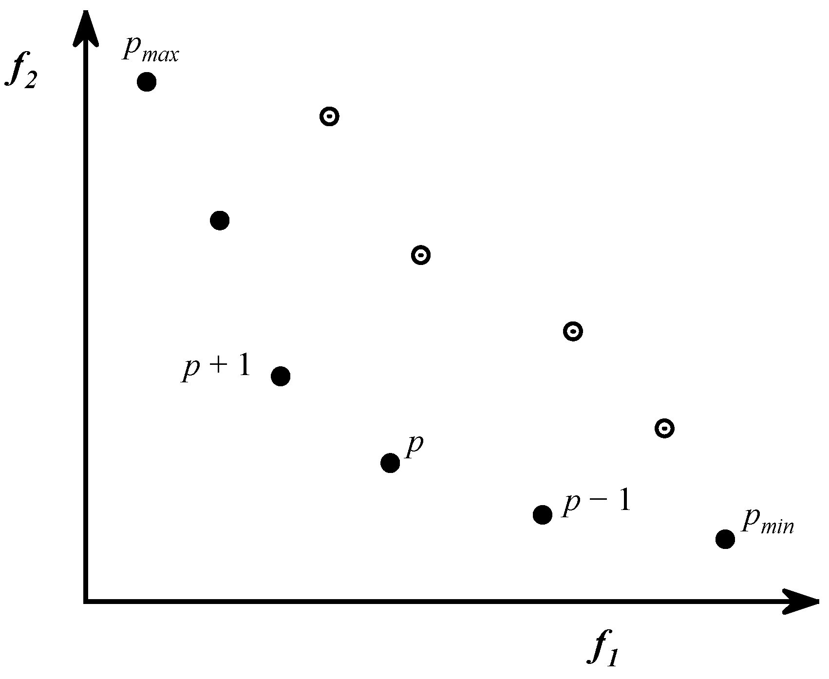
NSGA-II uses the crowding distance operator to replace the previous sharing function method, which ensures the criteria for selecting excellent individuals in the same non-dominant rank, ensures the diversity of individuals in the population, and is conducive to the selection, crossover, and variation of individuals in the entire interval. For the concept of crowding distance defined by NSGA-II, the double objective function is taken as an example to explain, as the Pareto rank set of the double objective function is shown as a curve (Figure 5) in the graph. As shown in the figure, for the bi-objective problem, for the current solution p (black dot p in the figure), the crowding distance is defined as the perimeter of the quadrangle formed by its adjacent solutions p − 1 and p + 1. Note that when drawing, this quadrangle should not contain other solutions other than p. For the boundary solution (the black points pmax and pmin in the graph), we count the crowding distance as infinite. It can be seen that for a solution, the farther the crowding distance, the more sparse it is around this solution, and choosing such a solution is beneficial to maintaining the diversity of the population.
Similarly, for the three-objective function optimization problem involved in this paper, the obtained Pareto level set is shown as a concave surface in the three-dimensional graph; then for one of the solutions p, its crowding degree pdis is defined as
3.4. Crowded Comparison Operator
After non-dominant sorting and density estimation, each individual in the group has two attributes: (1) non- dominant rank prank; (2) crowding degree pdis, where the non-dominant grade pran = 1 is the highest. For crowding degree, to a certain extent, the smaller the crowding distance of a solution, the more crowded the solution is by other solutions. For two solutions with different non-dominant ranks, the solution with the lower rank value tends to be chosen. When two solutions have the same rank, they tend to choose the solution with the larger crowding distance or the smaller crowding degree. The crowding comparison operator is used to select solutions to achieve a wider Pareto optimal solution distribution.
3.5. Selection, Crossover, and Mutation
- (1)
- Selection
Inspired by “survival of the fittest” in nature, individuals with higher fitness have a greater chance of being passed on to the next generation, while those with lower fitness have a lower chance. Various selection methods exist, including roulette selection, ranking selection, best individual preservation, and random league selection, among others. In this study, the “best individual preservation” method is employed for selection.
- (2)
- Crossover
The crossover operation simulates the cross transposition of chromosomes in nature and is used to generate new individuals, which determines the global search ability of the algorithm. The standard NSGA-II algorithm uses the analog binary crossover operator, and the formula for the k + 1 generation of individuals is as follows [15]:
where and is the k + 1 generation individual generated after the crossover; and is the selected k-th generation individual; βqi is the evenly distributed factor, which is calculated as follows:
where ui is a random number belonging to [0, 1); η is the cross-distribution index, generally defined as 20~30. The value of η will affect the distance between the generated individual and the parent individual.
- (3)
- Mutation
Mutation is a genetic mutation that simulates an organism and is used to produce a new individual, just like crossover. The mutation operator of the standard NSGA-II algorithm is a polynomial mutation operator, and the calculation formula of the k + 1 generation individual is as follows [15]:
where is the selected individual of the k-th generation; is the k + 1 generation individual obtained by the mutation operation of pk; and are the upper and lower bounds of the decision variables, respectively; is calculated by the following formula:
where rk is the uniformly distributed random number in [0, 1]; ηm is the exponent of variation distribution.
3.6. Elite Strategy
The NSGA-II algorithm introduces elite strategy to achieve the purpose of retaining excellent individuals and eliminating inferior individuals. By mixing parent and child individuals to form a new group, the elite strategy expands the selection range when producing the next generation of individuals. Representing the parent population as P, where the number of individuals is n, and the child population as Q, the steps are as follows:
(1) Merge the parent population and the child population to form a new population. Then, the new population can be divided into M Pareto levels by non-dominant sorting.
(2) To generate new parents, first put the non-dominant individuals of Pareto level 1 into the new parent population, then put the individuals of Pareto level 2 into the new parent population, and so on.
(3) If all the individuals of grade k are put into the new parent set, the number of individuals in the set is less than n; and if all the individuals of grade k + 1 are put into the new parent set, the number of individuals in the set is greater than n. Then the crowding degree is calculated for all the individuals of grade k + 1, and all the individuals are arranged in descending order according to the crowding degree. Then all the individuals with rank greater than k + 1 could be eliminated.
(4) Place the individuals in rank k + 1 into the new parent set one by one in the order arranged in step 3 until the number of individuals in the parent set is equal to n, and then eliminate the remaining individuals in rank k + 1.
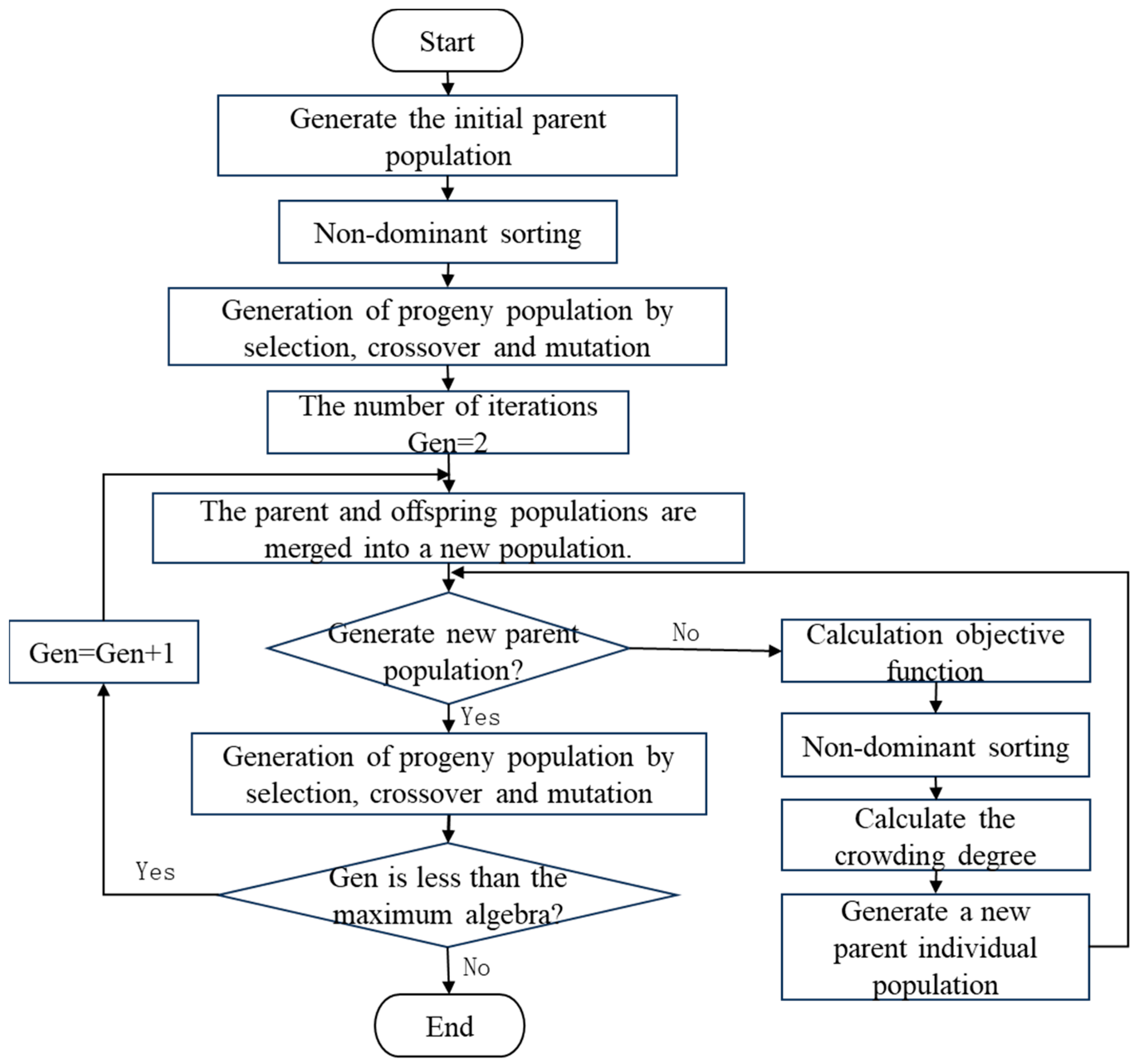
3.7. Algorithm Implementation Steps
The above algorithm is calculated through written code, and the calculation process and steps are shown in Figure 6.
4. Optimization of Calculation Results
The authors attempted to seek suitable parameter values during the model establishment and debugging stage, but manually adjusting the parameters, waiting for simulation results, and comparing experimental data were cumbersome and labor-intensive steps, and there was a high probability that the optimal parameter value could not be found. This is also an important reason for parameter optimization in this study. The author selected a set of manually adjusted parameter groups with good agreement between the results and experimental data as the initial parameter group (Table 2) to compare the matching effect of the optimized parameter group and verify the effectiveness of the parameter optimization model.
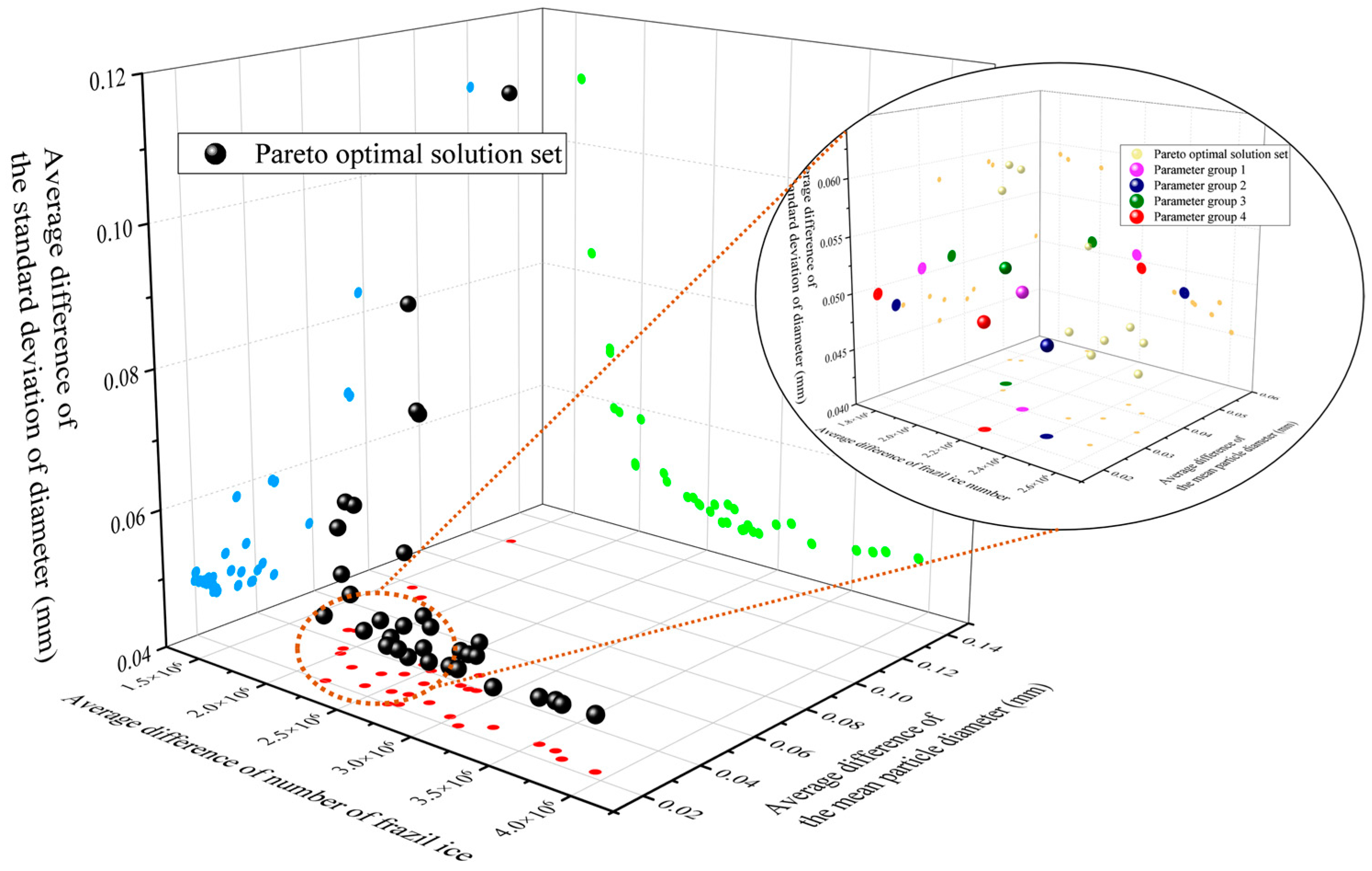
Figure 7 is a Pareto front curve of the three objective functions with the minimum average difference between the calculation results of the ice evolution model and the experimental observation results. The Pareto frontier curve obtained by optimizing the model in this study is an L-shaped spatial curve, which shrinks near the (0,0,0) coordinates and expands away from the (0,0,0) coordinates. Therefore, there are obviously a series of optimization parameter groups, and the average difference in frazil ice number, mean particle diameter, and the standard deviation of diameter are small; that is, the calculated results of the model are in good agreement with the experimental observation results. The optimization parameter values of each group are shown in Table 2. Figure 8 shows the comparison of water temperature, the number of frazil ice particles, average particle diameter, and standard deviation of diameter from experimental observation, calculated by initial parameter values and optimization parameter group 2.
Figure 8 shows the comparison curves between the simulation results and experimental results of frazil ice evolution corresponding to two parameter groups. It can be clearly seen that the improved frazil ice evolution model in this study is in good agreement with the experimental results and superior to previous models, especially in the evolution of ice quantity (Figure 1). This proves the accuracy and effectiveness of the frazil ice evolution model established in this study. Figure 8 also qualitatively shows the difference between the evolution process of frazil ice corresponding to the two groups of parameters and the experimental observation results. Intuitively, it seems difficult to see the specific difference between the three. Therefore, the differences among the three groups were further quantitatively calculated, and the average difference rate MAPE between the corresponding results of the initial and optimization parameters and the experimental observation results was obtained:
where is the calculated value of the objective function; is the experimental observation value. The average difference rate between the corresponding results corresponding to the initial value of the parameter and the optimized value and the experimental observation results is shown in Table 3. It should be explained that the author separately listed the average difference rate in the 600–1000 s period in Table 3 because during this period, the amount of frazil ice changes the most, and water temperature, number of particles, and the mean value and standard deviation of particle diameter are all in the stage of drastic evolution. Before 600 s, the number of frazil ice is very small, whether it is experimental observation or the simulation calculation result. The number of frazil ice shown in MacFarlane’s paper is on the order of 10 quadratic, and then according to the experimental conditions, the number in the whole calculation domain is expanded to seven times 10. Then, the error of the data obtained by manual extraction under this operation will also increase, so the experimental data obtained by the author may be inaccurate when there is very little frazil ice in the first 600 s. Therefore, taking them as the control data will affect the accuracy of the results.
According to the comparison curves shown in Figure 8, the curves of mean and standard deviation of frazil ice particle diameter corresponding to the optimization parameter values seem to be more consistent with the experimental observation results, but the curves of water temperature and number of particles cannot directly show whether the optimization parameter values are better than the initial parameter values. The average difference rate shown in Table 3 clearly compares the degree of agreement between the corresponding results of the two groups of parameters compared with the experimental results. Compared with the initial parameters, the optimization parameters of group 2 increase the difference rate of water temperature by 3.81%, decrease the difference rate of quantity by 4.21%, mean particle diameter by 35.73%, and standard deviation of diameter by 31.46%. For the period of 600–1000 s, the optimization process is more obvious, and the difference rate of water temperature is reduced by 0.68%, the difference rate of number of particles is reduced by 36.87%, the mean particle diameter by 35.34%, and standard deviation of the particle diameter by 57.14%. Compared to the other optimization groups, the results corresponding to the optimized parameters of group 2 are in the best agreement with the measured results. In addition to the corresponding water temperature process, the optimization value is slightly worse than the initial parameter values, the coincidence degree of the corresponding number of particles, mean particle diameter, and the standard deviation of diameter of the optimization value is better than that for the initial parameters, and the optimization degree is more obvious.
5. Discussion
5.1. The Improvement of the Frazil Ice Evolution Model
Compared to previous models, the improved frazil ice evolution model proposed in this article improves the initial seeding part, the ice particles collision, and the flocculation/breakup part. The following will further discuss these parts.
- (1)
- Initial Seeding
As described in Section 2.2, previous models simplified the initial seeding process of frazil ice. Wang and Doering [5] assumed that a certain number of ice nuclei were uniformly distributed in water at the beginning of the evolution process. Hammar and Shen [6] determined initial seeding as a fixed generation rate. However, there are still doubts about how these methods for determining the number of ice nuclei can be applied in actual situations, as the natural conditions of rivers and channels are complex. In the ice nucleation rate formula (Formula (5)) proposed in this article, parameter k is considered as a meteorological factor, and its value affects the maximum supercooling of the water temperature (Figure 9), thereby impacting the point at which frazil ice quantity starts to increase. The range of k values in Table 1 from 50 to 60 can be considered under ideal meteorological conditions (no wind, no rain or snow). For other meteorological conditions, such as rain, snow, strong winds, etc., more measured data will be needed in future research to determine the k value.
- (2)
- Ice Particles Collision Frequency and Flocculation/Breakup
In the Hammar and Shen [6] model, the particle collision frequency and result is related to volumetric sizes of the colliding particles, the turbulent dissipation rate, and velocity of the colliding particles. Svensson and Omstedt [4] also calculated the number of second nuclei from collision by the ice particle collision frequency, but it was assumed that one collision between particles would produce only one nucleus. This processing method differs from the actual physical process. Therefore, the author further improves the judgment of collision results (flocculation or breakup), including no repetition of particle collision count statistics, volume conservation before and after collision, and no uniqueness of collision results. The parameters introduced in this section include the stable particle size interval, the calibration coefficient of particle collision frequency, and the breakup calibration coefficient. From the calculation results of the evolution process, it can be seen that the upper limit of the stable particle size interval and the breakup calibration coefficient KC have a significant impact on the change in frazil ice quantity (Figure 10 and Figure 11), as these two parameters directly affect the process of ice particle collision and breakup, thereby affecting the change in frazil ice quantity.
5.2. Selection of Optimization Parameters and Objective Functions
The optimization parameters in this paper are determined according to the specific analysis of the influence on the evolution process of frazil ice, which mainly include air–water heat exchange coefficient hwa, ice nucleation coefficient k, stable particle size range, frazil ice thickness-to-width ratio Std, initial value of collision frequency calibration coefficient sequences M1, and collision fragmentation calibration coefficients KB and KC. Among them, the air–water heat exchange coefficient hwa has a positive correlation with the rate of water temperature reduction, the coefficient of ice nucleation coefficient rate k has a negative correlation with the maximum subcooling degree of water temperature, and the upper and lower limits of the stable particle size interval have a negative correlation with the maximum value and the stable value in the final period of the change process of the number of frazil ice, but the lower limit has a small impact. The initial value of the collision frequency calibration coefficient series M1 is negatively correlated with the number of frazil ice. The collision fragmentation calibration coefficients KB and KC are positively correlated with the number of frazil ice, of which KB has little influence.
Among these parameters, the air–water heat exchange coefficient hwa and ice nucleation coefficient k both affect the process of water temperature changes. The influence of k value on water temperature has been explained in Section 5.1. The influence of the air–water heat exchange coefficient hwa on water temperature is shown in Figure 12. The coefficient hwa mainly affects the supercooling rate of water temperature, and the larger the heat transfer coefficient, the faster the supercooling rate of water temperature. However, the air–water heat exchange coefficient hwa is determined according to specific conditions. Figure 13 shows the process curve of water temperature and number of particles obtained by MacFarlane’s laboratory experiments of frazil ice evolution. In the period when the number of frazil ice is small (the first 600 s in this working condition), the water temperature drops linearly, and the linear slope is approximately φ. At this time, due to the small number of frazil ice during this period, M, Qwi can be approximated as 0, and ρw, Cw, Awa, Ta are constant in the formula for calculating the time-course change of water temperature obtained by heat balance (Formulas (2) and (3)). Therefore, it can be deduced that the water temperature Tw is positively correlated with the heat exchange coefficient hwa (Formula (22)), and the time-course change of water temperature is the linear slope of water temperature cooling rate φ shown in Figure 13. Therefore, when the cooling rate of water temperature under the current working condition is obtained, the heat exchange coefficient hwa of water and gas can be determined. So, hwa is not considered within the scope of optimization parameters. Finally, seven parameters except hwa are selected as optimization parameters.
where φ is the slope of the water temperature decline process line.
The water temperature, the number of frazil ice particles, and the mean and standard deviation of particle diameter are the main observation objects of the evolution of frazil ice in order to achieve the best agreement between the simulation results and the observation results, that is, to quantify the minimum difference between the above four time-course results and the experimental observation results at each moment. At the same time, NASG-II has a good effect in solving low-dimensional optimization problems [24] because with the increase in the objective dimension of the optimization problem, the number of non-dominated individuals in the population increases exponentially, making it difficult to distinguish between good and bad individuals in the Pareto domination relationship, so three objectives need to be selected for optimization. From the physical process point of view, when the external temperature and the water-external heat exchange rate are constant, the water temperature change is affected by the water–ice heat exchange, so when the frazil ice characteristics data (quantity, mean and standard deviation of particle diameter) are well fitted, the difference in the water temperature process will be small. Moreover, the range of water temperature variation is in the order of 10−2, which makes the difference between the simulated results and the test results smaller. Therefore, this study selected the average difference between the number of frazil ice particles, the mean particle diameter, and the standard deviation of diameter of the simulation results and the experimental observation results as the optimization objective function.
5.3. The Water Temperature Difference of Each Optimization Parameter Group on the Pareto Front
When discussing the selection of optimization objective function in the previous section, it is considered that the difference in water temperature under different parameter groups is small, so the average difference in water temperature is not taken as the objective function. Figure 14 and Table 4 respectively show the degree of agreement between the simulation water temperature process corresponding to each parameter group in the Pareto front under this optimization condition and the experimental results. According to the data, the average difference value of the water temperature process obtained by each parameter group is between 0.005 °C and 0.008 °C, and the difference is small, which validates the authors’ decision to discard the average difference value of water temperature as the objective function before. However, the maximum difference value of water temperature shows that the maximum difference in water temperature corresponding to the four optimal parameter groups reached 0.04–0.05 °C (Table 4). The maximum difference occurred at t = 760 s, which was at the stage of “explosive” growth of the number of frazil ice and recovery of water temperature. From the perspective of the physical process of the evolution of frazil ice, as analyzed above, when the change process of the number of frazil ice is similar, the water temperature process will not produce much difference. Therefore, the analysis shows that even if the total amount of frazil ice in the calculation domain is similar, the amount of different particle size groups may be different, and the water–ice heat exchange rate of frazil ice with different particle size will eventually lead to the difference in water temperature process. It can be seen that the simulation results of the evolution model of frazil ice should not only be compared with the total number but also pay attention to the quantity distribution of each particle size group in the process.
5.4. Discussion of the Optimal Parameters Obtained from the Optimization Model
The optimization results show that the agreement between the optimization parameter corresponding results and the observation results is better than that for the initial parameter values. The further comparison between the initial parameter group and the optimized parameter group shows that the ice nucleation rate coefficient k in the optimized parameter group is higher than that in the initial parameter group, so the water temperature reaches the maximum supercooling degree in advance, and the maximum supercooling degree decreases. However, with the increase in k, the time of rapid growth of number of particles corresponding to the optimal parameter group is advanced, which is in better agreement with the experimental observation results. However, the increase in k value will lead to the increase in explosive growth rate and peak value of particles number, which is also the reason for the decrease in DB-max, KB and KC in the optimal parameter group, belonging to the result of automatic selection of the optimization model.
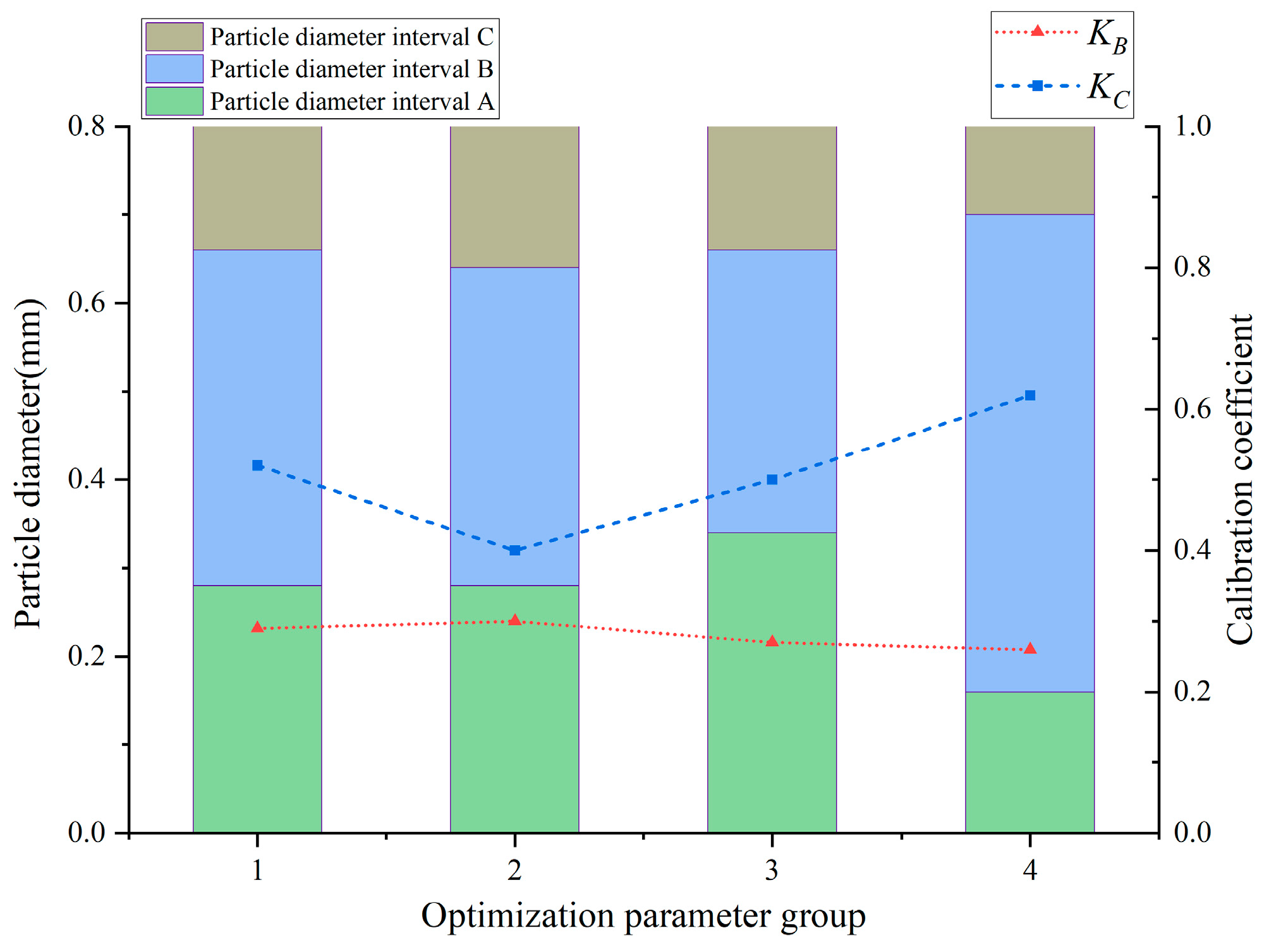
The above analysis also determined the coupling effect of other parameters on the process of the number of frazil ice particles. Figure 15 shows the distribution of the upper limit DB-max, lower limit DB-min, and collision fragmentation calibration coefficients KB and KC of the stable particle size interval that have a significant impact on the evolution of the number of particles in the four optimization parameter groups, where the stable particle size interval B is the stable particle size interval, the partition particle diameter of the intervals B and A is the lower limit DB-min, and the partition particle diameter of the intervals B and C is the upper limit DB-max. The average difference rate between the change process of the number of frazil ice particles corresponding to the four groups of optimization parameters and the test results during the period of drastic change is 17~20% (Table 3), so it can be considered that the number process calculated by the four groups of parameters is basically the same. However, under this condition, the values of each group of parameters shown in Figure 15 are not the same, wherein the coefficient KC has the same trend with the upper limit value DB-max. It is analyzed that the change in the upper limit value DB-max causes the change in the number of frazil ice in the interval C, so the optimization model is bound to adjust the collision fragmentation calibration coefficient KC (in the model of the evolution of frazil ice, collision fragmentation happened between the ice in the interval C colliding with each other) to meet the objective function of the number of ice particles. There is little difference in the size of coefficient KB in the four parameter groups, and the value of KB in Group 4 is slightly smaller than that in the other three groups. The analysis suggests that the range of interval B in Group 4 is large, that is, there is a large amount of frazil ice in interval B, and the model optimization finds a small value of KB to meet the quantity objective function.
6. Conclusions
(1) The improved frazil ice evolution model established in this study is in good agreement with the experimental results and superior to previous models, especially in the evolution of ice quantity. This proves the accuracy of the improved frazil ice evolution model.
(2) In this paper, a multi-objective optimization model of frazil ice evolution parameters based on NSGA-II is established. Compared with the experimental observation results, the corresponding results of the optimization parameters reduce the water temperature difference rate by 5.75%, the quantity difference rate by 39.13%, the mean particle diameter difference rate by 47.64%, and the standard deviation of particles diameter difference rate by 56.84% in the intense evolution stage of frazil ice evolution, which proves that the multi-objective optimization design model in this paper is effective and feasible for determining the parameters of the frazil ice evolution process.
(3) The initial values of parameters obtained are a set of optimal parameters, which has taken a lot of time and energy. The optimization model can greatly improve the efficiency of parameter optimization and avoid artificial parameter adjustment to obtain local optimal parameters.
(4) By comparing the differences in calculation results corresponding to optimization parameters, it is considered that there is still room for improvement in the frazil ice evolution model. Due to the limited observation data of frazil ice evolution experiments, it is impossible to simulate and compare the evolution process of multi-flow conditions at present. In the future, when the data are sufficient enough, the optimal parameters will be determined by optimizing the model, and then the frazil ice’s evolution process theory will be improved through the reverse analysis of the optimal parameters.
Author Contributions
Writing—original draft preparation, Y.C.; Funding Acquisition, J.L. and X.Z.; Writing—Review and Editing, X.Z.; Investigation, D.Y. All authors have read and agreed to the published version of the manuscript.
Funding
The authors are grateful for financial support from the Program of the National Natural Science Foundation of China with grant number U20A20316 and 51909186.
Data Availability Statement
The original contributions presented in the study are included in the article, further inquiries can be directed to the corresponding author.
Acknowledgments
The authors would like to thank the reviewers and editors whose critical comments were very helpful in preparing this article.
Conflicts of Interest
The authors declare no conflict of interest.
References
- Chen, Y.; Lian, J.; Zhao, X.; Guo, Q.; Yang, D. Advances in Frazil Ice Evolution Mechanisms and Numerical Modelling in Rivers and Channels in Cold Regions. Water 2023, 15, 2582. [Google Scholar] [CrossRef]
- Omstedt, A.; Svensson, U. Modeling supercooling and ice formation in a turbulent Ekman layer. J. Geophys. Res. 1984, 89, 735–744. [Google Scholar] [CrossRef]
- Osterkamp, T.E.; Gosink, J.P. Frazil ice formation and ice cover development in interior Alaska streams. Cold Reg. Sci. Technol. 1983, 8, 43–56. [Google Scholar] [CrossRef]
- Svensson, U.; Omstedt, A. Simulation of supercooling and size distribution in frazil ice dynamics. Cold Reg. Sci. Technol. 1994, 22, 221–233. [Google Scholar] [CrossRef]
- Wang, S.M.; Doering, J.C. Numerical simulation of supercooling process and frazil ice evolution. J. Hydraul. Eng.-ASCE 2005, 131, 889–897. [Google Scholar] [CrossRef]
- Hammar, L.; Shen, H.T. Frazil evolution in channels. J. Hydraul. Res. 1995, 33, 291–306. [Google Scholar] [CrossRef]
- Ye, S.Q.; Doering, J. Simulation of the supercooling process and frazil evolution in turbulent flows. Can. J. Civ. Eng. 2004, 31, 915–926. [Google Scholar] [CrossRef]
- Wang, S.M.; Doering, J.C. Development of a mathematical model of frazil ice evolution based on laboratory tests using a counter-rotating flume. Can. J. Civ. Eng. 2007, 34, 210–218. [Google Scholar] [CrossRef]
- Yan, Q.; Huang, W. Spaceborne GNSS-R Sea Ice Detection Using Delay-Doppler Maps: First Results from the U.K. TechDemoSat-1 Mission. IEEE J. Sel. Top. Appl. Earth Obs. Remote Sens. 2016, 9, 4795–4801. [Google Scholar] [CrossRef]
- Yan, Q.; Huang, W.; Moloney, C. Neural Networks Based Sea Ice Detection and Concentration Retrieval from GNSS-R Delay-Doppler Maps. IEEE J. Sel. Top. Appl. Earth Obs. Remote Sens. 2017, 10, 3789–3798. [Google Scholar] [CrossRef]
- Yan, Q.; Huang, W. Sea ice sensing from GNSS-R data using convolutional neural networks. IEEE Geosci. Remote Sens. Lett. 2018, 15, 1510–1514. [Google Scholar] [CrossRef]
- Naali, F.; Alipour-Fard, T.; Arefi, H. Spatial reslution sensitivity analysis of classifciation of sentinel-2 images by pre-trained deep models from big earth net database. Int. Arch. Photogramm. Remote Sens. Spat. Inf. Sci. 2021, XLIII-B3-2021, 87–92. [Google Scholar] [CrossRef]
- Ghiasi, Y.; Duguay, C.R.; Murfitt, J.; Asgarimehr, M.; Wu, Y. Potential of GNSS-R for the Monitoring of Lake Ice Phenology. IEEE J. Sel. Top. Appl. Earth Obs. Remote Sens. 2024, 17, 660–673. [Google Scholar] [CrossRef]
- Srinivas, N.; Deb, K. Multiobjective Function Optimization Using Nondominated Sorting Genetic Algorithms. Evol. Comput. 1994, 2, 1301–1308. [Google Scholar] [CrossRef]
- Deb, K.; Agrawal, S.; Pratap, A.; Meyarivan, T. A fast elitist non-dominated sorting genetic algorithm for multi-objective optimization: NSGA-II. Lect. Notes Comput. Sci. 2000, 1917, 849–858. [Google Scholar] [CrossRef]
- Kurek, W.; Ostfeld, A. Multi-objective optimization of water quality, pumps operation, and storage sizing of water distribution systems. J. Environ. Manag. 2013, 115, 189–197. [Google Scholar] [CrossRef]
- Wang, H.; Du, L.; Ma, S. Multi-objective open location-routing model with split delivery for optimized relief distribution in post-earthquake. Transp. Res. Part E Logist. Transp. Rev. 2014, 69, 160–179. [Google Scholar] [CrossRef]
- Hussain, I.; Parveen, A.; Ahmad, A.; Qadri, M.Y.; Qadri, N.N.; Ahmed, J. NSGA-II-based design space exploration for energy and throughput aware multicore architectures. Cybern. Syst. 2017, 48, 536–550. [Google Scholar] [CrossRef]
- Che, Z.H.; Chiang, T.A.; Lin, T.T. A multi-objective genetic algorithm for assembly planning and supplier selection with capacity constraints. Appl. Soft Comput. 2021, 101, 107030. [Google Scholar] [CrossRef]
- Wang, Y.; Xie, J.; Xu, Y.P.; Guo, Y.; Wang, Y. Scenario-based multi-objective optimization of reservoirs in silt-laden rivers: A case study in the Lower Yellow River. Sci. Total Environ. 2022, 829, 154565. [Google Scholar] [CrossRef]
- Khare, V.; Yao, X.; Deb, K. Performance scaling of multi-objective evolutionary algorithms. In Proceedings of the Evolutionary Multi-Criterion Optimization (EMO 2003), Faro, Portugal, 8–11 April 2003; Springer: Berlin, Germany, 2003; pp. 376–390. [Google Scholar]
- Purshouse, R.C.; Fleming, P.J. Evolutionary many-objective optimisation: An exploratory analysis. In Proceedings of the Congress on Evolutionary Computation (CEC 2003), Canberra, ACT, Australia, 8–12 December 2003; pp. 2066–2073. [Google Scholar]
- Wagner, T.; Beume, N.; Naujoks, B. Pareto-, aggregation-, and indicator-based methods in many-objective optimization. In Proceedings of the Conference on Evolutionary Multi-Criterion Optimization (EMO 2007), Matsushima, Japan, 5–8 March 2007; Springer: Berlin, Germany, 2007; pp. 742–756. [Google Scholar]
- Brockhoff, D.; Zitzler, E. Objective reduction in evolutionary multiobjective optimization: Theory and applications. Evol. Comput. 2009, 17, 135–166. [Google Scholar] [CrossRef]
- Von Lücken, C.; Barán, B.; Brizuela, C. A survey on multi-objective evolutionary algorithms for many-objective problems. Comput. Optim. Appl. 2014, 58, 707–756. [Google Scholar] [CrossRef]
- Li, B.; Li, J.; Tang, K.; Yao, X. Many-objective evolutionary algorithms: A survey. ACM Comput. Surv. 2015, 48, 1–35. [Google Scholar] [CrossRef]
- Deb, K.; Jain, H. An evolutionary many-objective optimization algorithm using reference-point-based nondominated sorting approach, Part I: Solving problems with box constraints. IEEE Trans. Evol. Comput. 2014, 18, 577–601. [Google Scholar] [CrossRef]
- Ishibuchi, H.; Imada, R.; Setoguchi, Y.; Nojima, Y. Performance comparison of NSGA-II and NSGA-III on various many-objective test problems. In Proceedings of the 2016 IEEE Congress on Evolutionary Computation, CEC 2016, Vancouver, BC, Canada, 24–29 July 2016; pp. 3045–3052. [Google Scholar]
- McFarlane, V.; Loewen, M.; Hicks, F. Measurements of the evolution of frazil ice particle size distributions. Cold Reg. Sci. Technol. 2015, 120, 45–55. [Google Scholar] [CrossRef]
- Holland, P.R.; Feltham, D.L.; Daly, S.F. On the Nusselt number for frazil ice growth—A correction to “Frazil evolution in channels” by Lars Hammar and Hung-Tao Shen. J. Hydraul. Res. 2007, 45, 421–424. [Google Scholar] [CrossRef]
- Daly, S.F. Frazil Ice Dynamics; US Army Cold Regions Research and Engineering Laboratory: Hanover, NH, USA, 1984. [Google Scholar]
- Osterkamp, T. Frazil Ice Formation: A Review. J. Hydraul. Div. 1978, 104, 1239–1255. [Google Scholar] [CrossRef]
- Osterkamp, T.E.; Gosink, J.P. An Investigation of Frazil and Anchor Ice: Formation, Properties, Evolution and Dynamics; Alaska University: Fairbanks, AK, USA, 1985; pp. 1–18. [Google Scholar]
- Chow, R.; Mettin, R.; Lindinger, B.; Kurz, T.; Lauterborn, W. The importance of acoustic cavitation in the sonocrystallisation of ice—High speed observations of a single acoustic bubble. In Proceedings of the 2003 IEEE Ultrasonics Symposium, Honolulu, HI, USA, 5–8 October 2003; pp. 1447–1450. [Google Scholar]
- Clark, S.; Doering, J. Laboratory Experiments on Frazil-Size Characteristics in a Counterrotating Flume. J. Hydraul. Eng. 2006, 132, 94–101. [Google Scholar] [CrossRef]
- Clark, S.; Doering, J. Experimenta0l investigation of the effects of turbulence intensity on frazil ice characteristics. Can. J. Civ. Eng. 2008, 35, 67–79. [Google Scholar] [CrossRef]
- Matoušek, V. Frazil and skim ice formation in rivers. In Proceedings of the 11th International Symposium on Ice, Banff, AB, Canada, 15–19 June 1992; pp. 1–22. [Google Scholar]
Figure 1.
Comparison between time variations of calculated quantity of frazil ice and actual observation results [5].
Figure 1.
Comparison between time variations of calculated quantity of frazil ice and actual observation results [5].

Figure 2.
Schematic diagram of frazil ice movement. (a) Ideal state and (b) actual state.

Figure 3.
Data from McFarlane et al. [29] for the evolution of frazil ice; turbulent dissipation rate 335.6 cm2/s3.
Figure 3.
Data from McFarlane et al. [29] for the evolution of frazil ice; turbulent dissipation rate 335.6 cm2/s3.

Figure 4.
Schematic diagram of frazil ice concept group based on diameter.

Figure 5.
Schematic diagram of individual crowding distance under double objective function.

Figure 6.
Parameter optimization calculation steps of frazil ice evolution model.

Figure 7.
Pareto frontier (black dots) of three-objective function (average difference in number, mean and standard deviation of particle diameter) for parameter optimization of frazil ice evolution model. The red, blue, and green dots represent the projections of the Pareto front on the XY, YZ, and XZ plane, respectively.

Figure 8.
Comparison diagram of (a) water temperature, (b) number of frazil ice particles, (c) mean and (d) standard deviation of particle diameter calculated from experimental observation, initial parameter group, and optimization parameter group 2.
Figure 8.
Comparison diagram of (a) water temperature, (b) number of frazil ice particles, (c) mean and (d) standard deviation of particle diameter calculated from experimental observation, initial parameter group, and optimization parameter group 2.


Figure 9.
The influence of parameter k on the calculation results of water temperature.

Figure 10.
The influence of the upper limit of the stable particle size interval on the calculation results for number of ice particles.
Figure 10.
The influence of the upper limit of the stable particle size interval on the calculation results for number of ice particles.

Figure 11.
The influence of the breakup calibration coefficient KC on the calculation results for number of ice particles.
Figure 11.
The influence of the breakup calibration coefficient KC on the calculation results for number of ice particles.

Figure 12.
The influence of parameter k on the calculation results for water temperature.

Figure 13.
Curve of water temperature and number of frazil ice process observed by MacFarlane’s frazil ice evolution experiment [29] (φ is the slope of water cooling process line).
Figure 13.
Curve of water temperature and number of frazil ice process observed by MacFarlane’s frazil ice evolution experiment [29] (φ is the slope of water cooling process line).

Figure 14.
Distribution of average difference value of number of frazil ice-water temperature obtained from each optimization parameter group.
Figure 14.
Distribution of average difference value of number of frazil ice-water temperature obtained from each optimization parameter group.

Figure 15.
Distribution of upper and lower limits of stable particle diameter interval DB-min, DB-max, and crushing calibration coefficients KB and KC in four optimization parameter groups.
Figure 15.
Distribution of upper and lower limits of stable particle diameter interval DB-min, DB-max, and crushing calibration coefficients KB and KC in four optimization parameter groups.


Table 1.
Optimizing the constraint range of variables.
| Parameter Range | k | Lower Limit Value of Stable Particle Size Range DB-min | Upper Limit Value of Stable Particle Size Range DB-max | Thickness-to-Width Ratio Std | Initial Value of Collision Frequency Calibration Coefficient Sequences M1 | Collision Fragmentation Calibration Coefficient KB | Collision Fragmentation Calibration Coefficient KC |
|---|---|---|---|---|---|---|---|
| Minimum value xi-min | 50 | 0.1 | 0.6 | 0.1 | 0.1 | 0 | 0.3 |
| Maximum values xi-max | 60 | 0.6 | 1.2 | 0.01 | 1 | 0.3 | 1 |
Table 2.
Parameter values in the initial parameter group and the optimization parameter group.
| Group | k | DB-min | DB-max | Std | M1 | KB | KC |
|---|---|---|---|---|---|---|---|
| Initial group | 53 | 0.4 | 0.8 | 0.1 | 0.9 | 0.32 | 0.7 |
| Optimization group 1 | 58 | 0.28 | 0.66 | 0.1 | 0.68 | 0.29 | 0.52 |
| Optimization group 2 | 60 | 0.28 | 0.64 | 0.1 | 0.66 | 0.3 | 0.4 |
| Optimization group 3 | 58 | 0.34 | 0.66 | 0.1 | 0.6 | 0.27 | 0.5 |
| Optimization group 4 | 58 | 0.16 | 0.7 | 0.1 | 0.86 | 0.26 | 0.62 |
Table 3.
The average difference rate between the frazil ice evolution results corresponding to the initial parameter group and the optimization group and the experimental observation results.
Table 3.
The average difference rate between the frazil ice evolution results corresponding to the initial parameter group and the optimization group and the experimental observation results.
| Water Temperature | Number of Frazil Ice Particles | Mean Particle Diameter | Standard Deviation of Diameter | |||||
|---|---|---|---|---|---|---|---|---|
| Average Difference Rate (%) | Average Difference Rate for 600–1000 s (%) | Average Difference Rate (%) | Average Difference Rate for 600–1000 s (%) | Average Difference Rate (%) | Average Difference Rate for 600–1000 s (%) | Average Difference Rate (%) | Average Difference Rate for 600–1000 s (%) | |
| Initial parameter group | 14.68 | 35.10 | 140.06 | 29.29 | 7.64 | 8.46 | 44.94 | 61.01 |
| Optimization group 1 | 15.49 | 33.64 | 127.83 | 19.74 | 5.53 | 6.16 | 33.75 | 37.90 |
| Optimization range (%) | −5.52 | 4.16 | 8.73 | 32.60 | 27.62 | 27.19 | 24.90 | 37.88 |
| Optimization group 2 | 16.69 | 33.08 | 126.62 | 17.83 | 4.37 | 4.43 | 30.39 | 26.33 |
| Optimization range (%) | −13.69 | 5.75 | 9.60 | 39.13 | 42.80 | 47.64 | 32.38 | 56.84 |
| Optimization group 3 | 15.12 | 34.50 | 128.81 | 18.93 | 6.54 | 7.60 | 33.68 | 37.63 |
| Optimization range (%) | −3.00 | 1.71 | 8.03 | 35.37 | 14.40 | 10.17 | 25.06 | 38.32 |
| Optimization group 4 | 15.05 | 35.54 | 138.89 | 17.88 | 3.87 | 3.48 | 33.45 | 38.41 |
| Optimization range (%) | −2.52 | −1.25 | 0.84 | 38.96 | 49.35 | 58.87 | 25.57 | 37.04 |
Table 4.
The degree of agreement between the water temperature process corresponding to the four groups of optimization parameters and the experimental results.
Table 4.
The degree of agreement between the water temperature process corresponding to the four groups of optimization parameters and the experimental results.
| Optimization Parameter Group | Average Difference Rate of Water Temperature (%) | Average Difference in Water Temperature (°C) | Maximum Difference Value of Water Temperature (°C) |
|---|---|---|---|
| 1 | 15.49 | 0.0057 | 0.044 |
| 2 | 16.69 | 0.0062 | 0.042 |
| 3 | 15.12 | 0.0057 | 0.043 |
| 4 | 15.05 | 0.0060 | 0.048 |
Disclaimer/Publisher’s Note: The statements, opinions and data contained in all publications are solely those of the individual author(s) and contributor(s) and not of MDPI and/or the editor(s). MDPI and/or the editor(s) disclaim responsibility for any injury to people or property resulting from any ideas, methods, instructions or products referred to in the content. |
© 2024 by the authors. Licensee MDPI, Basel, Switzerland. This article is an open access article distributed under the terms and conditions of the Creative Commons Attribution (CC BY) license (https://creativecommons.org/licenses/by/4.0/).
Share and Cite
MDPI and ACS Style
Chen, Y.; Lian, J.; Zhao, X.; Yang, D. Parameter Optimization of Frazil Ice Evolution Model Based on NSGA-II Genetic Algorithm. Water 2024, 16, 1232. https://doi.org/10.3390/w16091232
AMA Style
Chen Y, Lian J, Zhao X, Yang D. Parameter Optimization of Frazil Ice Evolution Model Based on NSGA-II Genetic Algorithm. Water. 2024; 16(9):1232. https://doi.org/10.3390/w16091232
Chicago/Turabian StyleChen, Yunfei, Jijian Lian, Xin Zhao, and Deming Yang. 2024. "Parameter Optimization of Frazil Ice Evolution Model Based on NSGA-II Genetic Algorithm" Water 16, no. 9: 1232. https://doi.org/10.3390/w16091232
Note that from the first issue of 2016, this journal uses article numbers instead of page numbers. See further details here.